2.1 Dynamic Characterisation of Flexible Beams by Numerical Investigation

The numerical analysis uses a Cartesian co-ordinate system: x is the longitudinal axis (beam length direction), while y (out-of-plane vertical direction) and z (in-plane horizontal direction) are axis in the cross-section plane. The selected cross-sections have the following shapes: a) Rectangular [x-R], b) I [x-I] and c) U [x-U] shape. The dimensions and shape are reported in Table 1, Table 2 and Fig. 1, respectively. Each section is represented by using two parameters [1]: Γ = EI_y/EI_x and θ = J_t/I_x.

Table 1 Rectangular cross-section with 20 mm base, geometrical parameters

Table 2 I and U cross-section geometrical parameters: b, h, s and s_c in mm

Figure 1. Beam cross-section shapes.

2.2 Cross-Sections Analysis

The geometrical and material beam properties are as follows: Length: L=500 mm; Material: Aluminium; Density: ρ = 2710 kg m⁻³; Young’s Module: Y=73 GPa; Yield Stress: σ = 345 MPa. A simple rectangular cross-section beam (R-type) with 20 mm width and selected height are reported in Table 1. Figs. 2–4 display the natural frequencies obtained through numerical investigations performed using both linear (Euler-Bernoulli linear theory) and nonlinear (nonlinear FEM software ABAQUS^® by SIMULIA) analysis. Values have been normalized with respect to the linear frequencies. The edge and torsion frequencies show the important modal coupling due to deflection: with a tip displacement of 38% of the beam length a 70% reduction in the first edge frequency is manifested for the R-type section with thickness of 1 mm. Bending frequencies are less influenced by tip deflection. This is also the case for beams with I and U cross-sections and Figs. 5–7 show the numerical results. Also in these cases the modes mostly influenced by large deflection are edge and torsion. By assessing the nonlinear effects on the natural frequencies, it can be concluded that such behaviour depends on the cross-section geometry as well as two parameters Γ and θ. An example can be seen in Fig. 5, where both 1-U and 3-I show the same trend with different geometrical parameters. However, this holds true only for a single mode, i.e., 1-U and 3-I have same behaviour in the 1^st Torsion mode but are different in the other ones. Additionally, the investigation shows that for the I-type cross section and for increasing, larger variations in natural frequencies occur. Due to the significant difference in θ parameters between the two considered sections this does not appear for U-type cross section. Notwithstanding, these initial investigations clearly show the importance of taking large deflection nonlinearities into account.

Figure 2. (a) 1^st and (b) 2^nd nonlinear Edge frequencies, variation in % with respect to the linear case.R-type cross section.

Figure 3. (a) 1^st and (b) 2^nd nonlinear Bending frequencies, variation in % with respect to the linear case. R-type cross section.

Figure 4. 1^st Torsion frequencies, variation in % with respect to the linear case. R-type cross section.

Figure 5. 1^st Torsion frequencies, percent variation respect linear case. I- and U-type cross sections.

Figure 6. (a) 1^st and (b) 2^nd non-linear Edge frequencies, variation in % with respect to the linear case. I-and U-type cross sections.

Figure 7. (a) 1^st and (b) 2^nd nonlinear bending frequencies, variation in % with respect to the linear case.I- and U-type cross sections.

2.3 Experimental Investigation

Experiments are proposed in order to investigate and validate the numerical results presented in Section 2.2. The rectangular cross section is considered in the experimental campaign. The beam tip deflection is induced by changing the length of the test articles and by making use of the beam own weight. Other methods of generating beam deflections were explored but discarded for a number of reasons; a tip mass inducing a tip displacement would have changed the boundary condition at the tip and consequently the mode shapes and frequencies; on the other hand, the use of a distributed mass, would have been quite difficult to accurately assess. From the Euler-Bernoulli linear beam theory, the natural frequencies follow the relationship ${f_n} = {{\rm{C}}_{\rm{m}}}\cdot\beta _{\rm{n}}^2$ where C_m is function of the material and $\beta _{\rm{n}}^4 = \frac{{\mu \cdot \omega _{\rm{n}}^2 }}{{\rm{D}}}$. Remembering that the free vibration equation can be cast as ψ _,xxxx − β ^{Reference Brit, Ortega, Tigue and Scott4} ψ = 0, it is possible to obtain the eigenvalues of the system, namely λ _i= (β · L)_i, and a frequency index which is independent from the beam length. For the transverse and edge vibrations these frequencies are scaled with length-square, that is ${\tilde \tau _n} = {f_n}\cdot{{\rm{L}}^2}$, while for the torsion frequencies are scaled with length, that is ${\tilde \tau _{{t_n}}} = {f_{{t_n}}}\cdot{\rm{L}}$. While the frequency index will change its value for each length when considering the nonlinear case, this will not be the case for a linear analysis.

The linear behaviour in the experimental campaign is simulated by placing the beam vertically, such that the self-weight deformation would not affect the measurements. The comparison between numerical and experimental analysis is reported in the subsequent figures. Numerical predictions reported in Figs. 8–10 confirm that ${\tilde \tau _n}$ values at different length are always constant when the assumption of linearity holds valid (all results were normalized with the linear values at length 950 mm, both numerical and experimental). The nonlinear torsion analysis highlights an increase in the frequency ratio for shorter beams, while an opposite trend is noticeable for longer beams as the assumption of linearity breakdown. Good correlation is shown between numerical and experimental data. The minor discrepancy can be attributed to manufacturing imperfections, material property estimations, the position of the beam and the root clamp set-up. Because of such small discrepancy, in the bending mode there is only a very small visible difference between the linear and nonlinear analysis. Comparing linear experimental and numerical results for the 1^st bending frequency the error is less than 8%. Fig. 9 shows that the numerically estimated 1^st nonlinear bending frequency increases with the length of the beam while it decreases in the experiment. Considering the beam max length of 950 mm, the linearly estimated 1st bending frequency is 1.56 Hz, while its nonlinear counterpart is 1.47 Hz, i.e. the difference in % is only 5.77% (0.09 Hz). These findings do demonstrate that there are no significant changes between two experimental linear and nonlinear analyses which confirm the small sensitivity of the bending mode with respect to the tip displacement. Very good correlations between experiments and numerical results are also shown for all the other considered frequencies and modes. It is also worth reporting that there is a notable difference at a beam length station between 600 ÷ 700 mm from the root. Several analyses have been repeated to confirm the results and the variance is attributed to material or manufacturing imperfection in the aluminium beam.

Figure 8. Normalized ${\tilde \tau _n}$ parameter for bending linear and non-linear data.

Figure 9. Normalized $tilde \tau _n $ parameter for (a) bending linear and (b) non-linear data.

Figure 10 Normalized${\tilde \tau _n}$ parameter for (a) edge linear and (b) non-linear data.

3.1 Numerical Model

Numerical models have been generated to assess the wing dynamic behaviour. To consider the large deformation, both 3D and 2D numerical models by Abaqus^® are proposed. The 3D model was generated from a combination of hexahedral and tetrahedral elements, while for the 2D model just the shell elements were used. For this model a 3D deformable shell, obtained by solid extrusion, is considered. This shell represents the spar, which is the deformable part of the wing. The materials used for the model are different and all are defined by engineering constant. The number of element in the 3D model is about 5· 10⁷ while for the 2D shell model the significantly smaller number of element is 5·· 10³. The 2D model is computationally efficient and since the difference in the results was less than 5%, it was deemed to be acceptable for the analysis. Consequently, all the remaining analyses were carried out with the simplified 2D model. Through the thickness integration was carried out by Simpson method, with 5 thickness integration points. Rigid elements, linked to several references points, were defined to simulate the inertia properties of the wing in FE model. Using CATIA^® it was possible to identify the correct position of the center of gravity of each section; 25 reference points were created, one for each section that complete the wing. The position of these points corresponded to the centre of gravity of the spar in the experimental model. All properties, as the weight and the inertial properties of each section (I ₁₁, I ₂₂, I ₃₃), were added to these points. Taking into account that ABAQUS solves the model step by step, two different steps were defined. Since the aim of this work is to better understand the effect of the nonlinearities, the following approach is considered. For the linear cases in a single step frequencies and modal shapes are calculated, while, for nonlinear cases, during the first step, the structure is deformed under self-weight and external load, in the second step, the frequencies and the modal shapes are calculated. The static analysis is carried out using Newton or semi-smooth method, while the modal analysis is solved with Lanczos method, normalized by mass matrix.

3.2 Wing Dynamics

A number of experimental investigations are performed, to assess the behaviour of the wing in its linear and nonlinear states. The Polytec Scanning Laser Vibrometer (LSV) for the rapid non-contact vibration measurement is used to determine the wing dynamic modal properties, including bending/torsion and edge frequencies and mode shapes. The modal characterisation can assist in the design of any structure, helping to identify areas where design changes are needed. It can also predict the vibration characteristics of components and systems. The LSV uses the Doppler Effect and can make rapid and accurate measurements, substantially cutting down traditional modal testing costs. The development of a modal model, from either frequency response measurements or from a finite element model, is useful for simulation and design studies. For example, it can be used to perform structural dynamics modification; this is a mathematical process which uses modal data (frequency, damping and mode shapes) to determine the effects of changes in the system characteristics due to physical structural changes. All experimental wing setups (both linear and nonlinear) were fixed to a rigid steel plate, to eliminate any possible coupling effect between frequencies of the mounting frame and the interested structure frequencies. In the linear setup, to avoid geometrical nonlinearities which can be caused by the self-weight, the wing was mounted vertically; however, it is worth reporting that the effect of weight could have slightly increased the longitudinal stiffness of the structure due to the vertical stretching force. The shaker is positioned near the root, where the wing was rigidly constrained to simulate a cantilever configuration, as to excite the wing in the frequency range of interest. The Polytec software run the shaker, while the laser head is used to scan all grid points virtually positioned on the wing, and to extract FRFs at each scanned point. Mode shapes at the natural frequency are also computed at each FRF major peak. For bending, torsion, and edge frequencies different configurations are tested, by rotating either the wing or the LSV to carry displacement or velocities laser measurements in the designated direction.

Taking into account the wing assembly, numerical predictions still agree relatively well with the experimental tests. The proximity between bending and edge frequencies is noticeable, and for this wing can induce edge-bending flutter. Generally speaking this type of flutter is more common in highly flexible wing, contrarily to the classical flutter, which involves bending-torsion coupling. Table 3 reports the data collected from the numerical and experimental investigations. For the simple wooden spar, it was not possible to generate large deflections under self-weight, hence linear and non-linear natural frequencies were quite close. Fig. 12 shows the bending-torsion modes FRFs. Linear and nonlinear trends are quite similar, although the nonlinear results were slightly noisier above 150 Hz. Since the range of interest was below 100 Hz the nonlinear effects at high frequencies are not significant for this study. The SLV software is used to reconstruct mode shapes and facilitated the identification process of the modes of interest.

Table 3 Wing frequencies [Hz] – Linear and Non-Linear

Figure 12. Bending/torsion FRF, (a) Linear - Beam clamped on the shaker; (b) Linear – Shaker near wing root; [Peak at: 4.96, 27.34, 31.09, 78.91] Hz (c) Non-Linear – Beam clamped on the shaker [Peak at: 4.96,25.78, 29.30, 79.69] Hz. More details in Table 3.

The comparison between linear and nonlinear numerical analysis displays the coupling among edge modes with torsion. Indeed, Fig. 13b shows the existence of a coupling between the 1^st nonlinear edge mode and the torsion mode compared with the linear prediction displayed in Fig. 13a. Same consideration can be made comparing results in Figs. 14a and Fig. 14b which display respectively 2^nd linear and nonlinear edge mode. The bending and torsion modes are not displayed since are not coupled. Unfortunately it was not possible to reconstruct the edge mode shapes from the SLV experiment given the small thickness, hence no comparison can be made with the numerical edge modes.

Figure 13. 1^st Edge reconstructed mode, (a) linear and (b) nonlinear.

Figure 14. 2^nd Edge reconstructed mode, (a) linear and (b) nonlinear.

By using the “Half Power Point Method” structural damping has also been evaluated. These are:

• 1^st Bending: ζ= 0.0913; 2^nd Bending: ζ = 0.12

• 1^st Edge: ζ= 0.028; 2^nd Edge: ζ = 0.12

• 1^st Torsion: ζ= 0.0912

4.1 Aeroelastic Behaviour

Aeroelastic investigations were carried out on a wing at 0° AoA. The high-speed camera captured frames displaying dynamic response and flutter.

In a linear system, flutter is the point at which zero-damping (combined structural and aerodynamic) is displayed. Above flutter, an unbounded sinusoidal self-oscillation is exhibited. Real system are nonlinear and given the presence of a non-linear stiffness the vibrations remain constrained into a bounded oscillation, and the flutter condition leads to Limit Cycle Oscillation mode (LCO). The first manifestation of a critical condition (flutter) is a sinusoidal self-oscillation structural response with amplitude growing with increasing speed. It will be called V_cr1 the speed at which a first self-sustained oscillation (LCO) occurs while V_cr2 the speed at which the wing behaviour changes becoming more aggressive with an increase in frequency and amplitude.

Fig. 15 shows the complete response of the wing when the speed is increased and Fig. 16 illustrates the amplitude and frequency variation in time.

Figure 15. Wing dynamic response at the trailing-edge point.

Figure 16. (a) Frequency and (b) amplitude magnitude variations for increasing speed and time.

The experiment starts with an initial speed of 22 ms⁻¹, lower than V_cr1, and the speed is increased quasi-statically with a very slow rate as to minimize the influence of the ramp up.

When the first critical speed V_cr1 = 22.97 ms⁻¹ is reached, the aeroelastic behaviour changes, the oscillation amplitude suddenly increases and the wing entered in a self-sustained oscillation. With the increases in speed both the amplitude and the frequency increases. The frequency at 4 sec is 13 Hz, whereas at 22 sec is 14.3 Hz. The amplitude changes from around 20 mm (at t=0 sec) to 23.5 mm (at 22 sec).

The wind velocity is further increased until the wind speed reaches a second critical velocity, V_cr2 = 23.92 ms⁻¹ characterised by a sudden increase in LCO amplitude. Only few seconds of data are recorded at this speed to avoid wing destruction. Once this instability mechanism is triggered the air flow is reduced and, as shown in Figs. 15 and 16, after 23 sec, the dynamic response amplitude decreases. At V_cr2 there has been a critical variation both in frequency and in amplitude, with an amplitude increases of 52%, from 46 mm to 70 mm, whereas the frequency changes from 14.2Hz to 25Hz, i.e., 78%.

Fig. 17 shows the FFT before and after the V_cr2. Points before second critical condition consider a time interval between 6.9 and 7.4 sec. Two peaks after V_cr2 are caused by a point identification error.

Figure 17. FFT backward point (a) before V_cr2 t around 7s (b) after V_cr2.

The described analysis was conducted by considering the detected trailing-edge marker. Unfortunately the automatic detection routine was unable to accurately identify the other two-points. In spite of this, a trajectory was manually estimated for the leading-edge and elastic axis markers. By processing the single images by manual selection of markers it was possible to do a more detailed investigation. An investigation about the first LCO, that is above V_cr1, is also carried out. The time interval taken into account is very small (6.9 sec to 7.4 sec) but since the motion is periodic it is sufficient to display the main characteristics. Fig. 18 compares the three markers y amplitudes. The y-amplitude ratio about the rear and centre markers is η=1.247, a 25% increase. The y-amplitude difference between the two points (rear-point and centre-point) is caused by torsion. Fig. 19 displays the evolution of θ with the y displacement with a twist amplitude of 9° and centre point y amplitude (only caused by pure bending oscillation) of 15.8 mm.

Figure 18. Tip twist vs centre marker displacement, before V_cr2 - t ∊ [6.95, 7.35] s.

Figure 19. Three marker y displacement, before V_cr2 – t ∊ [6.95, 7.35] s.

Then further analysis was carried for the time interval capturing the transient form one to another critical condition. Time interval taken into account begins at 22 s and finishes at 22.9 s, for total of 250 frames. Fig. 20 shows the time-history of the twist measured at the tip and the amplitude increase when the V_cr2 is achieved is quite evident. The twist amplitude changed from ±20° to ±60° demonstrating that the trend in Figs. 15 and 16 may be influenced by the tip twist evolution and not by bending. From Fig. 21 it is possible to observe the variation of the centre point flapwise displacement vs θ. Being such marker very close to elastic axis, it seems clear that the maximum y-amplitude of the oscillatory motion decreases, as Fig. 22b, so for backward point the θ contribution influences the graphic as it can see in Fig. 22a showing the trajectories of three markers on wing tip. Forward point displays a decrease of amplitude being in the other side of backward point, so y-direction motion is out-of-phase with the theta motion. Interesting the centre point amplitude that is almost constant in the transition phase being the torsion effect negligible. At 22 s η=1.548 instead at 22.8 s, after the second critical speed, η=2.622 suggesting the twist influence in the y-amplitude oscillation of backward marker. Observing the pictures from High-Speed-Camera, the phenomenon appears to be clear. Last phenomenon that can be seen is the variation of the average position of the wing tip. Fig. 23 shows the change of position both in flapwise and chordwise direction of motion. Probably the motivation can be attributed to the very high angle-of-attack at which the wing is now subjected. At high angle rates, flow separation and dynamic stall dominate the wing dynamics and the wing does not respond promptly to the variation and AoA decreasing the pure bending oscillation (such phenomenon is also observed in^{(Reference Dowell and Tang9)}). Also in Fig. 23, the displacement toward the flow direction is illustrated. The centre point marker draws a figure eight shape and becomes more distinct with the beginning of the new condition at V_cr2. Moreover, the trajectory shift towards the edgewise direction (e.g. flow direction) since the aerodynamic force component in such direction increases for increasing AoA. Fig. 25 shows two frames before and after the V_cr2 in which it is clear the deflection towards the chordwise direction. With respect to modes participation in such condition, by analysing the high-speedcamera pictures, one can observe that above V_cr2 the motion is torsion dominated with a small edge contribution. In phase-plane portraits, in which a variable and its derivative are plotted, an indication of the oscillation motion typology is provided. It is observed in Fig. 24 that the oscillations are periodic and not chaotic, showing clearly the evolution of the two main physical parameters y and θ. For increasing speeds, the twist θ shows the greatest increase in both rotation and speed rotation whereas vertical amplitude decreases with increasing vertical speed. The figure also shows clearly that for increasing speeds the torsional displacement θ increases. As also shown in the earlier Fig. 21, while at t=7 s the torsional displacement θ ∈ [−12°, +8°] at t=22 s, just below V_cr2, θ ∈ [−20°, +20°]. Indeed, the torsion mode, influencing the AoA, becomes larger, while centre point amplitude (elastic axis) is almost constant with a decreasing trend. Therefore the total y amplitude of the backward point grows whereas remains equal for the centre point, less influenced by the torsion mode. Then with the increase of the speed the motion develops an increasing angle-of-attack with a constant bending oscillation until, reached the second critical condition, the AoA value is too high to keep the oscillation trend and a dynamic stall is exhibited due to flow separations.

Figure 20. Twist time-history at the wing tip, V ~ V_cr2 - t ∊ [22, 22.9] s.

Figure 21. Tip twist vs centre marker displacement - t ∊ [22, 22.9] s.

Figure 22. (a) Three marker y displacement (b) centre and backward marker amplitude - t ∈ [22, 22.9] s.

Figure 23. Centre marker trajectory - t ∈ [22, 22.9] s.

Figure 25. Wing position before and after flutter displays.

Figure 24. Phase-plane time histories for (a) twist and (b) flapwise bending, before V _cr2 - t ∈ [6.95, 7.35] s for c) twist and d) flapwise bending - t ∈ [22, 22.9] s.

4.2 LCO – Hysteresis

In post-flutter/LCO regime an hysteresis phenomenon is shown. Two experiments were conducted to verify the behaviour. The conditions taken into account are AoA 0° and −1°. The wind-tunnel velocity is increased up to a value just smaller than V_cr2 and then is decreased until the self-sustaining oscillation cease to exist. Unfortunately, in these wind-tunnel experiments it was not possible to record the wind speed, hence it is not possible to display the classical hysteresis graph as function of speed and amplitude. Pictorially, Fig. 26 illustrate the speed and amplitude trend of a general hysteresis manifestation. It is clear that the LCO disappears at a velocity (V₂) which is smaller than the one at which the LCO was triggered (V₁ = V_cr1). V_m is the maximum speed achieved in the experimental analysis. Unfortunately, the trend of the return curve is not known because of it was not possible to gather amplitude data linked with velocity data. Only two cases are showed in this investigation but several experimental results at different AoA were collected.

Figure 26. General hysteresis behaviour.

AoA 0°

Fig. 27 shows the LCO behaviour. At 5.8 s (V₁ = 22.97 ms⁻¹) a LCO is triggered. Speed is increased until 17 s, reaching the max value of V_m = 23.85 ms⁻¹, after which, for safety reasons, it is reduced. The LCO disappears at V₂ = 20.77 ms⁻¹, showing a clear difference between the initial and the final speed at which the LCO appears on a ramp up speed and disappears on a ramp down speed. By increasing the wind-tunnel speed both wing amplitude and frequencies increases. Velocity and frequency are related and at same value of velocity a single frequency value is obtained independently of being in the increasing or decreasing speed ramp. Interestingly, before the oscillation disappeared an unexpected growth of amplitude was displayed at 23 s and 25.5 s which was probably caused by inertial effects. Amplitude and frequency are displayed in Fig. 28.

Figure 27. LCO wing response, AoA=0°.

Figure 28. (a) amplitude and (b) frequency variation, AoA=0°.

AoA -1°

At AoA −1° the wing has a negative lift and the nonlinear LCO behaviour is triggered earlier. Initial speed at which the LCO is triggered on a ramp up speed is V₁ = 22.74 ms⁻¹ while it disappears on a ramp down speed at V₂ = 20.60 ms⁻¹. Maximum speed V_m is reached around 11 s. In previous analysis the motion was regular, instead with negative angle-of-attack the dynamics response changes. Fig. 29 shows the motion as time function. In this case a chaotic behaviour is quite clear and it is persistent until 18 s during the ramp down speed. Fig. 30 shows two FFTs, in the chaotic regime and in the regular LCO regime. The presence of nonlinearities is emphasize in the first of the two FFTs with evidence of super and sub harmonics centred at 5, 10, 15 and 20 Hz. In the LCO regime the dominating frequency is 10 Hz. It is worth noting here that the chaotic results might be due to the transient dynamics of the continuous change in speed, it was difficult to discern or to attribute to other changes. Future tests will assess further this behaviour by performing a number of constant speed investigations. Table 4 shows the speed values at different AoA. By increasing the AoA all speed parameters, V₁, V₂, and V_cr2, grow. Between −1° and 1°, V₁ (equal to V_cr1, i.e. first critical speed) and V₂ change of +2.5%, while V_cr2 changes of +5.5%. The results agree well with literature^{(Reference Brit, Ortega, Tigue and Scott4)}, in which an increase of such parameters is expected.

Figure 29. LCO wing response, AoA=−1°.

Figure 30. (a) Amplitude and (b) frequency variation, AoA=−1°. (a) time 6 ÷ 18 s (b) time 18 ÷ 34 s.

Table 4 LCO parameters at several AoA

5.1 Governing Equation

The governing equation for a generic three-dimensional undamped aeroelastic system is expressed as:

(1) $$[{\bf{M}}]\{ {\bf{\ddot x}}\} + [{\bf{K}}]\{ {\bf{x}}\} = \{ {\bf{F}}\} $$

where [M] is the mass matrix, [C] is the damping matrix, [K] is the stiffness matrix, {F} = {F ₁, F ₂, . . ., F _n}^T is the force vector and {x} = {x ₁, x ₂, . . ., x _n}^T is the displacement vector. The above aeroelastic system can either be solved in the frequency domain or the time domain to determine the flutter condition. While the former is an attractive option for aeroelasticians due to the relatively low computational intensity, its assumption of pure harmonic motion often renders the approach infeasible for capturing nonlinear aeroelastic phenomenon. Alternatively, treating the system in the time domain results in additional fidelity in determining the stability of the aeroelastic system, irrespective of the response or input conditions.

To reduce the number of degrees of freedom in the model, the displacement vector can be treated as the superposition of a subset of the natural modes, i.e.

(2) $$\{ {\bf{x}}\} = [\Phi ]\{ \xi \} $$

where [Φ] is the modal matrix (normalized by the mass matrix) and {ξ} = {ξ ₁, ξ ₂, …, ξN,}^T the modal coordinate vector. By substituting Equation (2) into Equation (1) and rearranging, the aeroelastic system is expressed in modal form:

(3) $$[{\bf{I}}]\{ \ddot \xi \} + \left[ {\matrix{ {\omega _1^2} & 0 & \ldots & 0 \cr 0 & {\omega _2^2} & \ldots & 0 \cr \vdots & \vdots & \ddots & \vdots \cr 0 & 0 & \ldots & {\omega _N^2} \cr } } \right]\{ \xi \} = {[\Phi ]^T}\{ {\bf{F}}\} $$

where [I] is the identity matrix and ω _i is the i ^th natural frequency. The modal system uses a truncated number of modes M << n, sufficient to capture the fundamental dynamics of the structure.

5.2 CFD Model

The general purpose finite volume ANSYS Fluent⁽¹⁾ R16 is used for higher-fidelity prediction of the transient aerodynamic loading. ANSYS Fluent solves conservation equations for mass and momentum (the Navier-Stokes equations), written in integral form as:

(4) $${{d\rho } \over {dt}} + \nabla (\rho {\bf{u}}) = 0$$

(5) $${d \over {dt}}\int_V \rho \phi dV + \oint_A \rho \phi u\,\, \cdot {\rm{ }}dA = \oint_A \Gamma \nabla \phi {\rm{ }} \cdot \,\,dA + \int_V {{S_\phi }} dV$$

where ρ is the fluid density, u is the flow velocity vector, is the diffusion coefficient, S _ϕ is the source term for the generic scalar ϕ and A is used to represent the boundary of the control volume, V.

The pressure and velocity are solved sequentially through the SIMPLE algorithm, and all advective terms of the transport equations are discretized by a second-order upwind scheme, whereas all diffusive terms are discretized by central differencing.

To accurately account for the effects of aerodynamic nonlinearities, such as boundary layer separation/dynamic stall at high twist angles, the two-equation k − ω SST model by Menter is used to predict the value of turbulent viscosity in the flow. This model is extensively used in both academia and industry most notably for its treatment of aerodynamic (undergoing an adverse pressure gradient) flows. For time integration, a dual time-stepping scheme is employed with second-order implicit temporal discretization. The time-step selected was based on temporal discretization of the highest natural frequency by 30 steps, with approximately 5-10 inner iterations to ensure residual convergence of 𝒪 (10⁻⁵).

5.2.1 Computational Grid

Due to the highly flexible structure, and in the interests of preserving mesh quality with the large scale deformations, a C-type structured grid, with domain extents of 15 chord lengths in all directions is generated. A grid of (80×40×25) elements is generated and deemed suitable suitable for grid sensitivity and verification with the first grid point corresponding to y ⁺𝒪(10). Fig. 31 illustrates isotropic views of the grids considered for the current study.

Figure 31. Computational grids generated for aeroelastic analysis.

5.2.2 Grid Deformation

The dynamic mesh model in ANSYS Fluent is used to implement the modal deformation of the wing. The motion description provided by the modal superposition solver is used to prescribe nodal displacements using the DEFINE_GRID_MOTION user defined function (UDF) macro. The components of the modes shapes considered are allocated to ANSYS Fluent memory and stored using the node memory N_UDMI macro. Fig. 32 shows pressure distribution of the wing undergoing modal deformation.

Figure 32. Contours of static pressure for the wing under modal deformations.

To ensure a sufficient grid quality during deformation, and to maintain a consistent grid resolution close to the deforming boundary, the diffusion-based smoothing technique is adopted. This model aims to have the interior elements absorb the mesh deformation, whilst aiming to preserve the mesh resolution and topology near the deforming boundary.

5.3 Aerodynamic Drag Polar

The aerodynamic performance of the wing is first considered using steady-state simulations at velocity U _∞ = 30 m/s. Fig. 33 presents the drag and pitching moment polars for the high aspect-ratio wing deformed by each mode shape at a generalized displacement of the ξ = 1 × 10⁻³. As expected, the first two modes have relatively little steady-state effect on the aerodynamic performance, due to the lack of any significant torsional component. The edge mode induces a larger pitching moment, which induces a twist of the wing, and is yet another indication of the nonlinear interaction of the torsion and edge modes. The torsional mode, produces an aggressive lateral shift in the drag polar (even at lower generalized displacements) due to the geometrical twist of the wing. The vertical shift is a result of massive separation from the leading edge.

Figure 33. Aerodynamic performance curves.

5.4 Static Trim Analysis

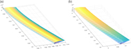
A characteristic of the flexible wing is the relatively large static trim position when exposed to loading. Performing a static trim analysis (essentially solving for Equation (3) but disregarding the acceleration and velocity terms) can assist in determining the contribution of weight relative to aerodynamic loading. For this analysis, at α = 0° and U _∞ = 30 m/s, the mesh is iteratively deformed in a quasi-steady framework until Δξ → 0, which for this system occurs after five iterations. The wing-tip deformations due to self-weight and total deformation are shown in Fig. 34(a) and the corresponding span wise isometric views are shown in Fig. 34(b). Under self-weight, the force is due to gravitational acceleration and is of the form of pure vertical loading, resulting in pure bending and a downwards shift of approximately 25% of chord. Under pure bending, the lift coefficient of the wing is similar to the undeformed configuration of c _L = 0.208. When exposed to aerodynamic loading, the pitching moment results in a slight torsional (nose-down) motion and an overall deformation of close to 38% of chord and the wing produces a down force of c _L = −0.044. Including the weight component results in a further reduction in the lift coefficient to c _L = −0.055, and an overall deformation of close to 62% of chord. Although the static trim position is primarily dependent on the aerodynamic loading, the indicial response analysis performed in the following subsection highlights the nonlinear scaling in transient effects at larger deformations. This further reiterates the inherent flexibility of high aspect-ratio wings and confirms the requirement to consider the wing self-weight for the subsequent dynamic aeroelastic analyses.

Figure 34. Static trim locations when exposed to various loads.

5.5 Response to Transient Impulse

Presented is the transient response to a step impulse in each mode shape to determine the transient aerodynamic shift in loading and the amount of aerodynamic damping. The responses are represented in terms of the generalized aerodynamic force [Φ]^T {F}. This is also known as the Indicial response of the aeroelastic system. The system is ramped from zero displacement to the fully deformed state (at t = 0.05 s) using a polynomial step input. As per the static analyses presented earlier, the final deformed state is equivalent to a generalized displacement of ξ = 1 × 10⁻³.

It is shown in Fig. 35 that the effect of edge motion (i.e. the second mode shape) is insignificant to the other mode shapes, especially compared with the torsion modes. This is due to the fact that only the drag force (i.e. F _x) is likely to be active here, and is a relatively small force component. A large transient effect is on the other hand seen for the first mode shape (pure bending). This is owing to the relatively large influence of the lift force component (i.e. F _y). A transient peak is observed before close to t = 0.05 s before the response damps and asymptotes to the quasi-steady value. As expected, due to the large geometrical twist, the largest variation in generalized loading is observed for the torsion modes. However, these modes also seemingly have less unsteady effects, as the response quickly asymptotes to the quasi-steady value with a negligible transient peak appearing.

Figure 35. Aerodynamic performance curves.

An insight into the non-linearity of the system can thus be observed by incrementally changing the value of Δξ and observing whether the response scales linearly. Fig. 36 shows the response of the generalized aerodynamic forces when the wing undergoes deformation by Φ₃, according to an incremental step impulse in the generalized displacement ξ ₃. The response seemingly begins to scale linearly with smaller values of ξ ₃, but essentially illustrates large transient effects as ξ ₃ > 2 × 10⁻³. The transient peak and aerodynamic damping progressively becomes more aggressive, suggesting the appearance of a strong aerodynamic non-linearity at larger displacements. To put in a clearer context to the reader, a generalized displacement of ξ ₃ > 2 × 10⁻³ is approximately equivalent to the wing deforming by 25% of the chord. Two interesting conclusions potentially arise from this study. The first, is that the system behaves in a rather stable fashion for small amplitudes, and transient instabilities scale non-linearly with uniform incremental changes in the impulse. The second, is that the inherent nonlinear nature of the system puts further doubt on the predictions of a frequency domain flutter analysis, especially in the context of using CFD to calculate the generalized aerodynamic force.

Figure 36. Transient aerodynamic response to modal impulse.

The non-linearity of the system is further evident from the response to a periodic input in the torsional mode, which is shown in Figs 37 and 38. At the lower value of ξ = 1.0 × 10⁻³, the response is close to a single harmonic. At the larger value of ξ = 2.0 × 10⁻³, the wing undergoes a dynamic stall due to massive flow separation. Multiple harmonics are now visible resulting in actuating and restoring forces. This is most likely a predominant reason for the appearance of sub-critical limit-cycle response for the flexible wings.

Figure 37. Transient aerodynamic response to periodic changes in torsional displacement.

Figure 38. Streamlines at peak displacement.

5.6 Linear flutter analysis

The iterative p-k method^{(Reference Hassig14)} is used to study the linear flutter solution and is a commonly used approach in industry^{(Reference Hodges and Alvin Pierce11)}. The aeroelastic system described by Equation (3) can be transformed to the frequency domain to give:

(6) $$\left({[{\bf{I}}]{p^2} + \left[ {\matrix{ {\omega _1^2} & 0 & \ldots & 0 \cr 0 & {\omega _2^2} & \ldots & 0 \cr \vdots & \vdots & \ddots & \vdots \cr 0 & 0 & \ldots & {\omega _N^2} \cr } } \right] - {1 \over 2}\rho {U^2}[{\bf{Q}}(ik)]{\rm{ }}} \right)\bar \xi = 0$$

where, [Q(ik)] is the aerodynamic influence coefficient (AIC) matrix obtained using the impulse response in Section 5.5. The frequency domain AIC is obtained from the time-history generalized aerodynamic forces [Φ]^T {F} using standard Fourier transform techniques^{(Reference Lee-Rausch and Baitina12)}.

The velocity-damping (V − g) and velocity-frequency (V − f) relation for each mode are shown in Fig. 39(a) and Fig. 39(b), respectively. The p-k method is strictly only valid for low damping g values and is accurate at the flutter point where g = 0 corresponding to velocity U _∞ = 23.8m/s for the torsional mode. The frequency corresponding to this mode at this velocity is 19.28Hz and is the flutter frequency. Since the wing experiences non-linear behavior structurally and aerodynamically, as shown earlier, it is expected that LCO is observed at a velocity and frequency below the values identified using linear techniques. Frequency domain techniques, such as the one used here, are limited and time domain methods would be required to identify critical speeds and frequency for LCO and flutter and is described in the following section.

Figure 39. Linear flutter analysis for the HALE wing.

5.7 Time domain analysis

The uncoupled equations, as described by Equation 3, representing the aeroelastic system are solved explicitly using a fourth-order Runge-Kutta time-advancement algorithm to obtain the generalized velocity $\mathop \xi \limits^ \bullet $ and displacement ξ. The mesh nodes can then be dynamically updated from time t to t + 1, according to the generalized displacement ξ _i of the i-th mode shape. The response using the RANS CFD model is discussed here in detail.

For the dynamic analysis, beginning from a converged steady solution, the wing is initially perturbed sinusoidally about its natural modes for one cycle. At the end of this forced cycle, the system is allowed to transiently evolve by its own self-induced loads as dictated by the solution of Equation (3) at time t. The response is computed for increasing values of the free stream velocity U _∞, to determine the location of the critical boundaries at an angle α = 0°.

When the velocity U _∞ < ULCO, a damped response is obtained, as shown in Fig. 40. The displacement at the wing-tip is monitored over time, as it converges to the trim value. This is evident from the modal displacement curves, which show the convergence of the base bending and torsion modes. The self-weight is the primary contribution to the bending displacement, whereas the twisting of the wing is dependent on the aerodynamic static load.

Figure 40. Damped response at U _∞ < U _LCO.

Within the range of U _LCO < U∞ < UF, a bounded limit cycle is obtained with the response shown in Fig. 41 where the time history of the leading and trailing edge tip displacements are shown in Fig. 41(a), the phase-plane of the vertical displacements and twist angles are shown in Fig. 41(b), the time history for the dominant modal co-ordinate shown in Fig. 41(c) and the Frequency Response Function (FRF) of the trailing edge tip displacement shown in Fig. 41(a) indicating peaks at the LCO frequency and its superharmonic. The amplitude of the limit-cycle is marginally dependent on the flow velocity. The tip rotation within this regime is θ= 15° which is slightly below that reported in the experimental study (Section 4.1) which was recorded at 17° < θ < 20°. As shown, this corresponds to a maximum torsional modal displacement of ξ3 = 1 × 10−3. This would suggest that the subcritical LCO is largely induced by the aerodynamic nonlinearity resulting from flow separation at higher twist angles. The normalised frequency response function is shown in Fig. 41(d). Small peaks are visible at each of the modal frequencies, with a strong peak visible at approximately fLCO ≈ 17[Hz], which is higher than that reported from the experimental study in Section 4.1.

Figure 41. Limit-cycle response at U _LCO < U∞ < UF.

At U _∞ >U _F, the wing tip deformation rapidly diverges and the amplitude is significantly increased. In fact, this condition generally results in severe degradation in quality of the mesh, due to severe twisting of the wing. Fig. 42 shows a sample time-history for the wing in flutter. The tip rotation within this regime increases to approximately θ = 90°, before the CFD solver diverges due to inverted elements.

Figure 42. Response forU _∞ >U _F.

The oscillation mode in flutter is typically dominated by torsion due to the significantly higher twist angle. As per the case U _LCO < U∞ < UF, the excitation in edge and bending modes is negligible by comparison. In Fig. 43, several still frames corresponding to a single oscillation cycle from the dynamic analysis are captured.

Figure 43. Still frames captured for one complete cycle of oscillation for U _LCO < U∞ < UF.

Table 5 documents the results for the dynamic response. The importance of capturing the aerodynamic field correctly is shown when comparing to the Euler result, which neglects profile drag of the wing, and fails to capture important phenomena such as the decambering effect and boundary-layer separation, which are also regarded as aerodynamic damping effects. Here, the loads experienced on the wing at a significantly lower velocity are required to initiate aeroelastic instabilities, and the critical margin U _LCO < U∞ < UF is reduced significantly.

Table 5 Results of the numerical aeroelastic model