3.1. Boundary integral equations

We introduce a complex variable $\zeta =\mathrm {e}^{-\mathrm {i}kz}$, where $k$ is the wavenumber and $z=x+\mathrm {i}y$. This transformation maps the physical flow domain $[-{\rm \pi} /k,{\rm \pi} /k]\times [-1,h]$ onto an annular region in the complex $\zeta$-plane (see, e.g. Papageorgiou & Vanden-Broeck Reference Papageorgiou and Vanden-Broeck2004). Since the complex velocity $w=u-\mathrm {i}v$ is an analytic function (u and v are the x and y components of the velocity), the Cauchy integral formula gives

(3.1)\begin{equation} w(\zeta)=\frac{1}{\mathrm{i}{\rm \pi}}\oint_C\frac{w(\zeta')}{\zeta'-\zeta}\,\mathrm{d}\zeta',\end{equation}

where $C$ represents the boundary of the upper or lower layer and $\zeta$ denotes a point on $C$. We can express $w$ in terms of the velocity modulus $q$ and the inclination $\theta$ as $w=q\mathrm {e}^{-\mathrm {i}\theta }$. Note that the relation between $\theta$ and the arclength parameter $s$ takes the formula of $\mathrm {e}^{\mathrm {i}\theta } = {\mathrm {d}z}/{\mathrm {d}s}$. Using these notations, (3.1) can be rewritten as

(3.2)\begin{equation} w(\zeta) ={-}\frac{k}{\rm \pi}\oint_C\frac{q}{1-\zeta/\zeta'}\,\mathrm{d}s.\end{equation}

Let $Y_+ = y(\sigma )+y(s)$, $Y_- = y(\sigma )-y(s)$, $X_+=x(\sigma )+x(s)$ and $X_- = x(\sigma )-x(s)$. Applying the Schwarz reflection principle to (3.2) for both fluid layers and taking the real part of equations, one then obtains

(3.3)\begin{align} &{\rm \pi} q_1(\sigma)x'(\sigma)/k\nonumber\\ &\quad ={-}\int_{0}^\alpha\left(\frac{q_1(s)(1-\mathrm{e}^{k(Y_+{+}2)}\cos(kX_-))}{1+\mathrm{e}^{2k(Y_+{+}2)}-2 \mathrm{e}^{k(Y_+{+}2)}\cos(kX_-)}-\frac{q_1(s)(1-\mathrm{e}^{kY_-}\cos(kX_-))}{1+\mathrm{e}^{2kY_-}- 2\mathrm{e}^{kY_-}\cos(kX_-)}\right)\mathrm{d}s\nonumber\\ &\qquad-\int_{0}^\alpha\left(\frac{q_1(s)(1-\mathrm{e}^{k(Y_+{+}2)}\cos(kX_+))}{1+ \mathrm{e}^{2k(Y_+{+}2)}-2\mathrm{e}^{k(Y_+{+}2)}\cos(kX_+)}-\frac{q_1(s)(1-\mathrm{e}^{kY_-} \cos(kX_+))}{1+\mathrm{e}^{2kY_-}-2\mathrm{e}^{kY_-}\cos(kX_+)}\right)\mathrm{d}s, \end{align}

(3.4)\begin{align} &{\rm \pi} q_2(\sigma)x'(\sigma)/k\nonumber\\ &\quad ={-}\int_{0}^\alpha\left(\frac{q_2(s)(1-\mathrm{e}^{kY_-}\cos(kX_-))}{1+\mathrm{e}^{2kY_-}-2\mathrm{e}^{kY_-}\cos(kX_-)}-\frac{q_2(s)(1-\mathrm{e}^{k(Y_+{-}2h)}\cos(kX_-))}{1+\mathrm{e}^{2k(Y_+{-}2h)}-2\mathrm{e}^{k(Y_+{-}2h)}\cos(kX_-)}\right) \mathrm{d}s\nonumber\\ &\qquad -\int_{0}^\alpha\left(\frac{q_2(s)(1-\mathrm{e}^{kY_-}\cos(kX_+))}{1+\mathrm{e}^{2kY_-}-2\mathrm{e}^{kY_-}\cos(kX_+)}-\frac{q_2(s)(1-\mathrm{e}^{k(Y_+{-}2h)}\cos(kX_+))}{1+\mathrm{e}^{2k(Y_+{-}2h)}-2\mathrm{e}^{k(Y_+{-}2h)}\cos(kX_+)}\right) \mathrm{d}s, \end{align}

where $\alpha$ denotes the total arclength of the interfacial wave in half period and the assumed symmetry property of waves has been used.

3.2. The Fourier method

Due to the periodicity and symmetry of the computed waves, we can express the unknown functions as Fourier series. For convenience, we introduce a normalised arclength parameter $\tau =s/\alpha$ and write the Fourier expansions as

(3.5) \begin{equation} \left.\begin{gathered} q_1(\tau)=\sum_{n=0}^{\infty}a_n\cos(n{\rm \pi} \tau),\quad q_2(\tau)=\sum_{n=0}^{\infty}b_n\cos(n{\rm \pi} \tau),\\ x(\tau)=c_0\tau+\sum_{n=1}^{\infty}\frac{c_n}{n{\rm \pi}}\sin(n{\rm \pi} \tau),\quad \eta(\tau)=d_0-\sum_{n=1}^{\infty}\frac{d_n}{n{\rm \pi}}\cos(n{\rm \pi} \tau). \end{gathered}\right\} \end{equation}

Truncating these series after $N$ terms gives $4N$ unknowns, namely $a_n$, $b_n$, $c_n$ and $d_n$ ($n=0,1,\ldots,N-1$). Putting them together with $F$, $B$ and $\alpha$, there are eventually $4N+3$ unknowns to be found. We evaluate (3.3) and (3.4) over the interval $[0,1]$ at $N$ equally spaced mesh points:

(3.6)\begin{equation} \tau_j=\frac{j-1}{N-1},\quad j=1,\ldots,N. \end{equation}

To avoid the singularity in the Cauchy integral formula, we introduce another set of mesh grids:

(3.7)\begin{equation} \tau_j^m=\frac{\tau_j+\tau_{j+1}}{2},\quad j=1,\ldots,N-1, \end{equation}

and calculate the integrals by applying the midpoint rule. The Bernoulli equation and the arclength equation

(3.8)$$\begin{gather} R q_2^2-q_1^2+2(R-1)\eta/F^2 = B, \end{gather}$$

(3.9)$$\begin{gather}x'^2+\eta'^2 = \alpha^2 \end{gather}$$

are satisfied at the mesh points $\tau _j$. Since the $x$-axis is fixed on the undisturbed interface level, we impose

(3.10)\begin{equation} \int_{0}^{1}\eta(\tau)x'(\tau)\,\mathrm{d}\tau=0\Rightarrow \sum_{n=1}^{N-1}\frac{c_nd_n}{2{\rm \pi} n}+ c_0d_0=0.\end{equation}

To close the system, we also need to give a definition of the wave amplitude $H$:

(3.11)\begin{equation} H = \eta(0)-\eta(1),\end{equation}

and prescribe the wave speed $c$ (which has been scaled to unity). There are different ways to define $c$. Following a widely used condition in surface gravity waves, we define $c$ as the averaged velocity in the lower fluid

(3.12)\begin{equation} \frac{k}{\rm \pi}\int_0^{{\rm \pi}/k}u_1(x,y=\text{const.})\,{\textrm{d}\kern0.06em x} ={-}1,\end{equation}

where $y=\text {const.}$ is an arbitrary horizontal line within the lower layer. The negative sign reflects the fact that the background current is from right to left in the moving frame of reference. Equation (3.12) can be rewritten in terms of $q_1$ by using the irrotationality condition

(3.13)\begin{equation} \frac{\alpha k}{\rm \pi}\int_0^1 q_1(\tau)\,\mathrm{d}\tau ={-}1\Rightarrow a_0\alpha ={-}\frac{\rm \pi}{k}.\end{equation}

In addition, a similar condition for $q_2$ is necessary for solving the problem:

(3.14)\begin{equation} b_0\alpha ={-}\frac{\rm \pi}{k}.\end{equation}

Although it is beyond the scope of this paper, it should be pointed out that the right-hand side of (3.14) can be an arbitrary constant, which can be thought of as giving different background current in each layer. Note that there are some extra conditions due to the symmetry of waves:

(3.15a–c)\begin{equation} x(0)=0,\quad \eta'(0) = 0,\quad \eta'(1)=0, \end{equation}

which are automatically satisfied owing to their Fourier representations. It is not difficult to verify that $c_0={\rm \pi} /k$ due to the spatial periodicity of waves. Finally, we have $4N+4$ (3.3)–(3.11) and (3.13)–(3.14) with only $4N+2$ unknowns. Therefore, we choose to drop the equations of (3.3) and (3.4) at $\tau =1$, and perform the Newton iteration to solve the system for given values of $R$, $k$, $h$ and $H$. The iteration process is repeated until the maximum residual error is less than $10^{-10}$. At first glance it seems dangerous to abandon two integral equations. However, our numerical results show that the maximum residual error of these two equations (denoted as $\delta$ hereafter) is of the order of $10^{-11}$ in most cases. Based on our numerical experience, $N=600$ usually gives accurate enough results and thus is used in most computations. For almost-limiting solutions, however, typically $1200$ Fourier modes are necessary to maintain appropriate accuracy and to ensure $\delta <10^{-4}$.

4.1. Validation

In table 1, we present results for $R=0.1$ and compare them with the works of Saffman & Yuen (Reference Saffman and Yuen1982) and Maklakov & Sharipov (Reference Maklakov and Sharipov2018). Since their results were obtained in the case when both layers are infinitely deep, we let $h=1$ and $k\gg 1$ to achieve a good approximation of their results, and after many tests it was found that $k=100$ is large enough to provide an excellent agreement. Note that these authors used a different length scale, $\sqrt {g/k}$, so their dimensionless wave amplitude reads $kH$. The dimensionless wave speed defined by Saffman & Yuen ($C_s$) and Maklakov & Sharipov ($C_m$) can be expressed as

(4.1a,b)\begin{equation} C_s = F\sqrt{k}\sqrt{\frac{1+R}{1-R}},\quad C_m =F\sqrt{k}. \end{equation}

Increasing $N$ up to $300$, we have nine correct decimals in comparison with Maklakov & Sharipov (Reference Maklakov and Sharipov2018) in most cases except for a few solutions very close to the limiting configuration. Though not explicitly shown in table 1, for most solutions $\delta = O(10^{-11})$, which demonstrates the validity of our numerical method. Even when $\delta$ increases to $O(10^{-6})$, seven correct decimals can be guaranteed with $N=300$.

Table 1. $C_s$ vs $kH$ for $R=0.1$, $h=1$ and $k=100$. The second and third columns are the results of Saffman & Yuen (Reference Saffman and Yuen1982) and Maklakov & Sharipov (Reference Maklakov and Sharipov2018), respectively.

4.2. Bifurcations and profiles

For any $R\in (0,1)$, there is a branch of solutions bifurcating from infinitesimal periodic waves, which always leads to overhanging solutions. When $h\geqslant 1$, the limiting profiles of these branches are of type I and their geometry relies on the values of $k$ and $R$. From a physical point of view, overhanging waves and associated limiting profiles would presumably suffer different instabilities (Kelvin–Helmholtz, Rayleigh–Taylor, etc.) and thus are difficult to be observed in experiments. However, our main concern here is the existence of limiting shapes which is separate from the question of instability. In figure 3, we show typical speed–amplitude bifurcation curves and related almost-limiting profiles for $h=1$. The bubble features a half-lens shape and becomes horizontally long and vertically thin when the value of $k$ is gradually decreased for a fixed $R$. Note that to compare the profiles with different wavelengths, we rescale the horizontal and vertical coordinates by multiplying $k$, as shown in figure 3(b). On the other hand, for a given wavenumber $k$, the bubble enlarges when the value of $R$ is increased, which is clearly demonstrated by figure 3(d). For general sets of parameters, bifurcation curves, along which almost-limiting profiles that are either of type I or of type II can be found. They appear qualitatively similar to those shown in figures 3(a) and 3(c). Guan et al. (Reference Guan, Vanden-Broeck, Wang and Dias2021) proposed a local model for the limiting configuration of type I for a small density ratio and calculated numerically profiles of the closed bubble. 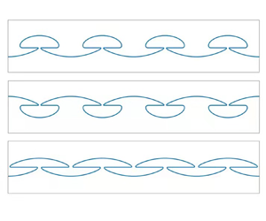The almost-limiting profiles computed with the primitive equations when both layers are deep ($h=1, k=100$) and solutions of the simplified model are shown in figure 4. For comparison purpose, we make sure they match at the wave crest and flat bottom. The density ratios are $R=0.1$, $0.2$ and $0.3$ from top to bottom and, as expected, the smaller density ratio gives a better agreement.

Figure 3. Typical speed–amplitude bifurcation curves and related almost limiting profiles. (a,b) $R=0.9$, $h=1$ and $k=1$ (blue), $k=2$ (red), $k=3$ (yellow). (c,d) $k=3$, $h=1$ and $R=0.2$, $0.5$, $0.9$. The corresponding almost-limiting profiles are plotted from top to bottom.

Figure 4. Comparisons between the almost-limiting solutions (blue) and solutions of the simplified model (red) from Guan et al. (Reference Guan, Vanden-Broeck, Wang and Dias2021). The parameters are chosen as $h=1$, $k=100$ and $R=0.1$, $0.2$, $0.3$ from panels (a–c).

When $R\to 1$, i.e. the Boussinesq limit, Grimshaw & Pullin (Reference Grimshaw and Pullin1986) predicted the existence of the type III solution. This is intuitively reasonable since gravity is negligible and the wave profile should be invariant after being turned upside down, if one omits the possible phase shift. Maklakov & Sharipov (Reference Maklakov and Sharipov2018) also supported this assertion but did not provide direct numerical evidence. In the top diagram of figure 5(a), we display an almost-limiting solution in the Boussinesq limit ($R=0.999999$) where $h=1$ and $k=100$ are used to approximate the condition that both layers are of infinite depth. This solution features a wave steepness of $0.1518{\rm \pi}$ and a wave speed of $1.141$ after being converted to the scaling of Grimshaw & Pullin (Reference Grimshaw and Pullin1986), which agree well with the corresponding values of $0.1411{\rm \pi}$ and $1.0923$ for the Stokes highest wave. It is also clear that the almost-limiting profile tends to become self-intersecting at both $x=0$ and $x=\pm {\rm \pi}/k$, hence yielding a limiting profile of type III. It is not surprising that the condition $k\gg 1$ is unnecessary to lead to such solutions, since the mirror symmetry with a possible phase shift relies only on the conditions $R\to 1$ and $h=1$ (recalling that the lower layer has a unit depth).

Figure 5. The bifurcation in the Boussinesq limit with $h=1$, $k=100$ and $R=0.999999$. (a) Three almost-limiting profiles that correspond to type III, type I and type II limits from top to bottom. (b) A new speed–amplitude bifurcation branch (red) bifurcates from the primary one (blue) at a secondary bifurcation point (black dot). The circle relates to type III limit and the asterisk corresponds to type I and type II limits.

However, it is found that the type III solution is not the only possible limiting profile in the Boussinesq limit. Other branches of solutions can arise through the secondary bifurcation mechanism as shown in figure 5(b). The blue curve is the primary branch bifurcating from infinitesimal periodic waves and the red circle denotes the almost-limiting configuration of type III (see the top figure of 5a). We check the Jacobian matrix along the primary branch and the solution is picked up as a candidate for the secondary bifurcation point if the matrix becomes nearly singular (interested readers are referred to Chen & Saffman (Reference Chen and Saffman1980) for more details). It is shown in figure 5(b) that a secondary bifurcation point is found to exist (black dot), from which two coincident branches of new solutions (red curve) arise terminating at the limiting profiles of type I and type II. The almost-limiting profiles are labelled by the asterisk and plotted in the middle and bottom figures of 5(a). Therefore, limiting configurations of types I–III coexist in the Boussinesq limit for $h=1$.

We take one of the secondary bifurcation branches as an example (the one which terminates at the type II limit, say) to explore its behaviour as $R$ varies. If the value of $R$ is slightly decreased, one can observe a separation of the secondary bifurcation curve from the primary branch as shown in figure 6(a). The isolated branch connects two limiting profiles labelled by a red dot and an asterisk, both of which are of type II. Three curves for $R=0.99$, $0.98$, $0.96$ are shown in figure 6(b), from which one can see a growing distance between the isolated branch and the primary one as $R$ is gradually decreased. Another striking feature is the shrinking tendency of these isolated curves as $R$ decreases (see figure 6c). For $R<0.86$, the new branch almost becomes a point, which indicates that these new solutions can exist only in a specific range of parameters. Therefore, it is also expected that the difference between the two limiting profiles at opposite ends of the isolated curve should gradually diminish as shown in figure 6(d), where blue and red curves correspond to dots and asterisks, respectively. It is worth mentioning that when the density ratio deviates from 1, the limiting configuration on the primary branch (labelled by a red circle) becomes type I, and the readers should not associate these markers (circle, dot and asterisk) with any specific type of limit in general.

Figure 6. Speed–amplitude bifurcation curves and related almost-limiting profiles with $h=1$ and $k=100$. (a) $R=0.999$. (b) $R=0.99$, $0.98$, $0.96$. (c) A series of new bifurcation branches shrinking from left to right. The leftmost curve bifurcating from a uniform flow corresponds to $R=0.92$. (d) Almost-limiting profiles with $R=0.92$, $0.88$, $0.86$ from top to bottom. Blue and red profiles correspond to dots and asterisks in panel (c), respectively.

As discussed above, the existence of the secondary bifurcation and of the branch separation phenomenon is found near the Boussinesq limit. One can then ask whether or not this novel bifurcation mechanism exists in other situations. We give a positive answer to this question based on the numerical results shown in figure 7. For $k=3$ and $R=0.5$, it is found that there is a special depth ratio $h_s$ for which three types of limiting solutions coexist and are linked via a secondary bifurcation point. Although the exact value of $h_s$ is not easy to determine, the numerical evidence shown in figure 7(a,b) strongly suggests $0.3601< h_s<0.3602$ in this case. As $h$ deviates from $h_s$, there are two types of branch separation depending on whether $h$ is decreasing or increasing. There are three sub-branches arising from the secondary bifurcation point at $h=h_s$. When $h$ is slightly below $h_s$, as shown in figure 7(a) for $h=0.3601$, the top sub-branch stays on the primary branch (blue line) while the bottom two sub-branches form a new curve with a sharp corner (red line) which isolates from the primary one. Figure 7(b) shows the result for $h=0.3602$ where the top and bottom sub-branches form a new curve (red line) breaking away from the primary branch (blue line). Note that although the two curves intersect at a common point in the parameter space as shown in figure 7(b), the two wave profiles at the intersection point are slightly different and this difference increases with $h$, indicating the branch separation phenomenon. A sequence of new bifurcation curves for different values of $h$ are plotted in figure 7(c), which clearly shows a transition near $0.36$. Almost-limiting waves akin to types I–III are labelled by the asterisk, circle and dot in figure 7(a) for $h=0.3601$, and corresponding typical profiles are plotted in figure 7(d) from top to bottom.

Figure 7. Speed–amplitude bifurcation curves and related almost-limiting profiles with $R=0.5$ and $k=3$. (a) $h=0.3601$. (b) $h=0.3602$. (c) A sequence of new bifurcation curves. (d) Three almost-limiting profiles corresponding to the asterisk, the circle and the dot in panel (a) from top to bottom.