


1. INTRODUCTION
“The First True Maps”, date back to late thirteenth century and are portolan charts for marine navigation (Beazley, Reference Beazley1904), regarded as “a unique achievement not only in the history of navigation but in the history of civilisation itself” (Campbell, Reference Campbell1987). The very first in-car navigation map appeared as rolled paper maps on one of the first dedicated in-car navigation systems Iter Avto in 1930, before debuting on portable media, cassette drives, in the mid-1980s (Newcomb, Reference Newcomb2013).
The 1990 Mazda Eunos Cosmo became the first car with a built-in Global Positioning System (GPS) navigation system with digital maps (Leite, Reference Leite2018). Digital maps were initially visualised like a paper map, but interactive and thus more easily retrievable. Importantly, digital maps allow updates from map data servers to be synchronised rapidly, reflecting the changing world in a timely manner. Furthermore, navigation systems use Global Navigation Satellite Systems (GNSSs) to determine vehicle position, performing map matching, calculating routes and giving directions to a driver. In fact, unlike most paper maps, digital maps are machine readable.
In the 2000s, enhanced digital maps were investigated to support Advanced Driver Assistance Systems (ADASs) and potentially automated driving (NextMap, 2002; EDMap, 2004). In enhanced digital maps, more accurate road geometry such as curvature, slope and richer road attributes, such as road width, lane width and speed limits have been included, by adding a layer of map data on the existing digital maps for ADAS. This is equivalent to Levels 1 and 2 of driving automation defined by SAE (Society of Automotive Engineers) (SAE, 2018).
Table 1. In-car navigation map evolution.

In 2010, the “high-definition map” concept was born at the Mercedes-Benz research planning workshop that led to the Bertha Drive Project (Herrtwich, Reference Herrtwich2018). In 2013, at the fruition of this project, an automated Mercedes Benz S-Class S 500 completed a 103 km journey covering urban and rural roads in fully autonomous mode, with a highly accurate and detailed Three-Dimensional (3D) map, that is, a high definition map (Ziegler et al., Reference Ziegler, Bender, Schreiber, Lategahn, Strauss, Stiller, Dang, Franke, Appenrodt, Keller, Kaus, Stiller and Herrtwich2014). In contrast with previous digital maps, this 3D map included new features for vehicle localisation and perception. As a participating partner in the project, a mapping company called HERE Technologies has since named its new map the “High Definition (HD) Live Map”, highlighting a near real time map update. However, this kind of map is more widely called an HD Map (tomtom.com, civilmaps.com). An HD Map is not just a navigation map but a powerful “sensor” that provides detailed information around and further around the corner to support ego vehicle perception once it is localised in the map (EDMap, 2004). Furthermore, it is part of the digital infrastructure for not only automated driving, but also a suite of applications such as urban planning, safety, smart cities and more (Dannehy, Reference Dannehy2016).
The HD Map has become a major research focus in recent years. While the race to deploy automated vehicles has broadened interest and accelerated the pace of research and development, there is a lack of comprehensive review of the overall conceptual framework and development status, which will be addressed in this study. The rest of this paper is structured as follows: Section 2 provides on overview of HD Map structure, functionalities, accuracy and standardisation developments, while Section 3 discusses HD Map models including the Road Model, Lane Model and Localisation Model. Approaches for HD Map mapping are outlined in Section 4. Section 5 introduces the HD Map-based vehicle localisation methods and presents a numerical analysis, which will be followed with the concluding remarks and recommendations.
2. HD MAPS: STRUCTURE, FUNCTIONALITIES, ACCURACY AND STANDARDS
Within the functional system architecture of an automated driving system (Figure 1), HD Maps are tightly associated with localisation functionality, interacting with the perception module and ultimately supporting the planning and control module (Matthaei and Maurer, Reference Matthaei and Maurer2015; Ulbrich et al., Reference Ulbrich, Reschka, Rieken, Ernst, Bagschik, Dierkes, Nolte and Maurer2017).

Figure 1. Functional system architecture of an automated driving system.
The different levels of automated driving tasks require that the world is modelled at different levels of details. HD Maps are not only the storage for globally referenced road networks and lane level details but also provide unique landmarks or the whole appearance of the surrounding environment to aid ego vehicle localisation. Both HD Maps and the pose of the ego vehicle are inputs to the perception module for world modelling, from which the planning and control module deduces actions and plans. On the other hand, the world model can also be fed back to make HD Maps up-to-date.
2.1. HD Map structure
An HD Map is defined as three layers for Bertha Drive (Ziegler et al., Reference Ziegler, Bender, Schreiber, Lategahn, Strauss, Stiller, Dang, Franke, Appenrodt, Keller, Kaus, Stiller and Herrtwich2014); BMW experimented with two layers: a semantic, geometric layer of lane models and a localisation layer (Aeberhard et al., Reference Aeberhard, Rauch, Bahram, Tanzmeister, Thomas, Pilat, Homm, Huber and Kaempchen2015). TomTom and HERE have launched HD Maps with similar three-layer structure (tomtom.com, here.com) (Table 2). The existing enhanced digital map is the common layer 1 in Table 2.
Table 2. Examples of layered structure of an HD Map.

The hierarchical structure of an HD Map with three consistently geo-referenced layers supports further vertical division, for example by degree of details (Kühn et al., Reference Kühn, Müller and Höppner2017) and horizontal division, for example geographically (Levinson et al., Reference Levinson, Montemerlo and Thrun2007) for implementation efficiency. This paper adopts HERE's terminology of Road Model, Lane Model and Localisation Model to refer to these three layers.
2.2. HD map functionalities
The Road Model is used for strategic planning (navigation). The Lane Model is used for perception and tactical planning (guidance) that takes the current road and traffic conditions into consideration. The Localisation Model is used to localise the ego vehicle in the map. The Lane Model can aid vehicle perception only if the ego vehicle is accurately localised in the map. Examples of these functionalities are illustrated in Figure 2.

Figure 2. Functionality of an HD Map. (a) Road Model supports navigation; (b) Localisation Model enables perception using Lane Model: the ego vehicle understands the presence of lane markings and an obstacle; (c) Lane Model supports tactical planning, for example, lane-changing manoeuvre.
2.3. HD Map accuracy
In the map community (Esri, 2018), absolute accuracy is generalised as the difference between the map and the real world, relative accuracy compares the scaled distance of objects on a map with the same measured distance on the ground.
The EDMap project has presented a more detailed definition (EDMap, 2004), which defines absolute accuracy as the maximum spatial deviation between the map geometry and the ground truth geometry; relative accuracy is calculated by first aligning these two geometries and it is the maximum spatial deviation between the aligned geometries. The consistency of the space deviations calculated for different corresponding point pairs determines the geometrical similarity and the correctness of relative accuracy (Figure 3).

Figure 3. Relative accuracy defined in EDMap (2004). (a) Incorrect relative accuracies: < 20 cm (orange) and > 20 cm (red) respectively; (b) Correct relative accuracies: < 2 0cm (orange) and > 2 0cm (red) respectively.
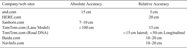
Table 3 lists the map accuracy proposed by some map providers from their web sites, which shows differences and the potential need for standardisation.
Table 3. The map accuracy parameters set by some notable map providers.
2.4. HD Map related standards
The International Organization for Standardization (ISO) Technical Committee (TC) 204 (ISO/TC 204) has published Geographic Data File (GDF) version 5·0 (ISO, 2011), which provides a base for both the capture of geographic content and exchanging it; GDF 5·1 will support automated driving. It has also published Local Dynamic Map (LDM) standard (ISO, 2018), the dynamic information stored in LDM including such information as weather, road or traffic conditions and the static data from HD Maps provides a comprehensive world model for ego vehicles.
Industry/government consortia such as Open AutoDrive Forum (OADF) (openautodrive.org) act as cross-domain platforms driving standardisations for automated driving. The Traveller Information Services Association (TISA) (tisa.org) is discussing the need to increase the Transport Protocol Experts Group (TPEGTM) traffic information accuracy to lane level. The Advanced Driver Assistance Systems Interface Specification (ADASIS) Forum (adasis.org) has just released version 3 of the ADASIS protocol allowing the distribution of HD Map data within the vehicle. Sensoris (sensor-is.org) is working on the standardisation of a vehicle-based sensor data exchange format for vehicle-to-cloud and cloud-to-cloud interfaces. Navigation Data Standard (NDS) Open Lane Model (NDS, 2016) and OpenDRIVE® (OpenDRIVE, 2015) are two industry standards related to HD Map data formats, which are compared with GDF file formats in Table 4. It is notable that only Road Model and Lane Model are covered; the Localisation Model standard is yet to be defined.
Table 4. Comparison of GDF, NDS Open Lane Model and OpenDRIVE®.

There are also regional or national efforts on developing HD Map standards. Japan has been working on the Dynamic Map, the Japanese version of the HD Map (en.sip-adus.go.jp). The formation of Automated Driving Map working Group of China Industry Innovation Alliance for the Intelligent and Connected Vehicles (CAICV) (caicv.org.cn) was announced in May 2018 with a vision for standardisation of automated driving and HD Maps in China.
3. HD MAP MODELS
The details of an HD Map, Road Model, Lane Model and Localisation Model, are discussed below.
3.1. Road Model
Road model in digital maps uses an ordered sequence of shape points describing the geometry of a polyline that represents the course of a road (Betaille and Toledo-Moreo, Reference Betaille and Toledo-Moreo2010). Each road section has its start and end nodes, which belong to the intersection at the start and end of the road (Figure 4).

Figure 4. Road Model (green polylines and yellow nodes) on top of Lane Model.
When using shape points to define curved road geometry, an increase in the density of intermediate points can achieve better accuracy but requires storing a large volume of information. Curvature definition with mathematical efficiency and simplicity has been introduced to extend the road model to support ADAS. Furthermore, hybrid road levels and some lane level geometry, with additional road properties and semantically richer attributes are being developed to model complex traffic rules. More significantly, the addition of slope information has added height information, that is, the third dimension of road geometry, in a traditional 2D navigation map (NextMap, 2002). Based on NDS (2016), EDMap (2004), NextMap (2002) and Kotei (2016), Table 5 gives examples of map content for ADAS and accuracy requirements. Accuracy requirements in EDMap (2004) were relative accuracy defined in Section 2.3 for ADAS applications. Those in NextMap (2002) and Kotei (2016) were defined for automated driving. However, the former refers to relative accuracy and the latter for absolute accuracy.
Table 5. Examples of map content for ADAS and accuracy requirements.

3.2. Lane Model
Lane models have been developed during some seminal automated driving events. The most famous lane map is the Road Network Description File (RDNF) for the Defense Advanced Research Projects Agency (DARPA) Urban Challenge. However, RNDF is 2D with a coarse lane model. Moreover, it was intentionally simplified as part of the competition instructions (DARPA, 2007).
A 3D lane model based on lanelet was used in the Bertha Drive project (Ziegler et al., Reference Ziegler, Bender, Schreiber, Lategahn, Strauss, Stiller, Dang, Franke, Appenrodt, Keller, Kaus, Stiller and Herrtwich2014). A lanelet is a drivable section of a lane that has left and right bounds with highly accurate geometrical proximation. Traffic regulations, including rules and information to assis in obeying the rules, are associated to the lanelets.
Expanding on these two examples, Lane Model includes:
3.2.1. Highly accurate geometry model
The lane geometry model largely determines the accuracy, storage efficiency and usability of Lane Model (Gwon et al., Reference Gwon, Hur, Kim and Seo2017), which covers not only the geometric structures of all lanes such as lane centre line, lane boundaries and road markings but also the underlying 3D road structure such as slope and overpass. Furthermore, it should be efficient for online calculations of items such as coordinates, curvature, elevation, heading and distance.
3.2.2. Lane attributes
Main lane attributes include lane centre lines, which are theoretical lines along the middle of the lanes, and lane boundaries with different shapes, colours and materials, which are captured in Lane Model as they are in the real world (Figure 5).
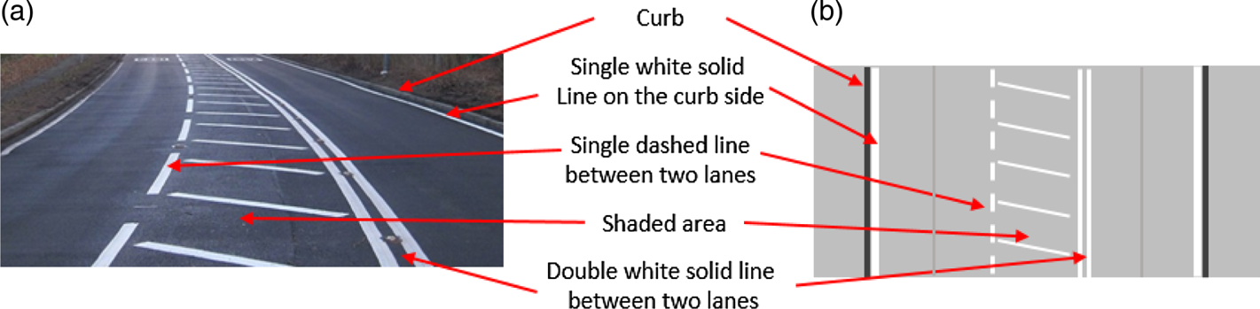
Figure 5. Lane boundaries in Lane Model. (a) A road; (b) Corresponding Lane Model.
3.2.3. Traffic regulations, road furniture and parking
Traffic regulations and relevant information/parameters may be embedded in other attributes, such as a road type for the lanes, which may implicitly indicate the default speed limit for the road. However, Lane Model has the capability to specify them for each lane or part of the lane. Just like physical objects such as parking slots and road furniture, it requires highly accurate location information when assigned to a lane, which can be modelled as part of the 3D road geometry (Zhang et al., Reference Zhang, Arrigoni, Garozzo, Yang and Cheli2016).
3.2.4 Lane connectivity
Lane connectivity describes the connection of the lanes or lane groups, which can be defined simply as a pair of predecessors and successors or as a complex intersection. The topological and semantic aspects of intersections are addressed by traffic matrices that define all manoeuvres aligning with traffic regulations. The geometrical aspect of lane connectivity is commonly addressed by “virtual lanes” that connect the exit and the entry control points, which can be modelled using the same geometrical lane model as normal lanes (NDS, 2016) or a different one (Guo et al., Reference Guo, Meguro, Kojima and Naito2014; Bauer, Reference Bauer, Alkhorshid and Wanielik2016) because the two fixed control points may affect the continuity of the curve (Figure 6).

Figure 6. An intersection with entry (blue dots) and exit (red dots) control points and the centrelines of virtual lanes (blue dashed arrow).
Table 6 lists some essential Lane Model contents summarised with information from map providers and standardisation organisations; accuracy requirements are given when applicable.

3.3. Localisation Model
The Localisation Model is designed for aiding vehicle localisation. It has been explored as feature-based or dense information-based approaches, affected by the sensors used, the characteristics of the environment, and the underlying algorithm (Grisetti et al., Reference Grisetti, Stachniss and Burgard2009), aligning with Lane Model content (Ziegler et al., Reference Ziegler, Bender, Schreiber, Lategahn, Strauss, Stiller, Dang, Franke, Appenrodt, Keller, Kaus, Stiller and Herrtwich2014).
3.3.1. Feature-based Localisation Model
A feature-based localisation model is generally stored as a graph, where nodes contain images and extracted 3D landmarks and edges contain the vehicle poses. Landmarks can be described by a feature descriptor to perform feature matching between a live image and the map. Figure 7(a) is an example of the landmark map used in Bertha Drive, which stores landmark 3D positions relative to corresponding vehicle poses with their respective image descriptors (Lategahn et al., 2013). The density of landmark maps can be too low to be useful in rural areas and a complementary map as shown in Figure 7(b) was created containing all the visible road markings with different attributes (solid, dashed, curb, stop line) (Schreiber et al., Reference Schreiber, Knöppel and Franke2013).

Figure 7. Localisation Model examples. (a) Landmark map with green landmarks and orange vehicle pose; (b) Road marking map with blue line segments (Lategahn et al., Reference Lategahn and Stiller2012; Schreiber et al., Reference Schreiber, Knöppel and Franke2013).
Feature maps are compact and efficient but require feature extractions in the process of offline map making and online localisation.
3.3.2. Dense information-based Localisation Model
A dense information-based localisation model can be further categorised as either location-based such as grid maps or view-based such as point cloud maps. Millimetre-wave radar and RGB-D (Red-Green-Blue-Depth) cameras are used to gather dense information for mapping (Guidi et al., 2010; Endres et al., Reference Endres, Hess, Sturm, Cremers and Burgard2014), while Light Detection and Ranging (LiDAR) is most widely used by leading mapping and automated driving companies such as HERE (here.com), TomTom (tomtom.com) and Google (waymo.com) etc.
2D grid maps have been explored over x-y planes (the ground) (Levinson et al., Reference Levinson, Montemerlo and Thrun2007) and x-z planes (vertical to the ground) (Li et al., Reference Li, Yang, Wang and Wang2016). In Figure 8(a), a flat road surface is assumed, and the grid cells are filled with an average infrared reflectivity value of LiDAR measurements (Levinson et al., Reference Levinson, Montemerlo and Thrun2007) which is subsequently replaced with a Gaussian distribution of the reflectivity values (Levinson and Thrun, Reference Levinson and Thrun2010). Both delivered localisation relative accuracy at the 10 cm level. Another approach is to use an occupancy grid. Figure 8(b) is an example of filling the grid cells with accumulated probabilistic information jointly defined by the distance to the road centre and the possibility of being occupied. Thus, 3D information from both sides of the road is compressed into a 2D grid map, which achieves localisation accuracy with a mean absolute error at the 40 cm level. However, 2D grid maps are not robust to environmental changes.

Figure 8. Examples of 2D grid map formats. (a) Reflectivity grid map (Levinson et al., Reference Levinson, Montemerlo and Thrun2007); (b) Occupancy grid map (colour denotes the distance to road centre) (Li et al., Reference Li, Yang, Wang and Wang2016).
2·5D map, a 2D map with height information, has been considered without dramatically increasing the size of the map. For example, Wolcott and Eustice (Reference Wolcott and Eustice2014) added z-height information in the 2D x-y reflectivity grid map to depict the height variation of the road; Morales et al. (Reference Morales, Tsubouchi and Yuta2010) added the estimated height to the commercially available 2D road centreline map for localisation in outdoor woodland environments. Furthermore, Wolcott and Eustice (Reference Wolcott and Eustice2015) proposed independently modelling z-height and reflectivity values to capture both structure and appearance, optimising using a multi-resolution search. Figure 9 illustrates the continued effort of improving 2D grid maps, from reflectivity to probabilistic maps and from 2D to 2·5D.

Figure 9. Continued effort of improvement. (a) 2D reflectivity grid map; (b) 2D probabilistic grid map; (c) 2D probabilistic grid map with height attribute; (d) 2·5D grid map. Only the i-th cell is annotated. Note: i = the index of the cell; z = height; r = reflectivity value; μ = mean; G = Gaussian distribution.
3D models can be found as point cloud maps represented by a set of data points typically latitude, longitude, altitude (Stewart and Newman, Reference Stewart and Newman2012) and intensity information (Xu et al., Reference Xu, John, Mita, Tehrani, Ishimaru and Nishino2017). Such point cloud maps can be textured with camera data (Pascoe et al., Reference Pascoe, Maddern, Stewart and Newman2015). The concern is that the memory requirement of a point cloud map grows exponentially when the mapping area gets bigger, which makes it not practical.
One of the challenges for the Localisation Model or HD Maps in general is how to reflect structural, seasonal or illumination changes in an environment. Churchill and Newman (Reference Churchill and Newman2013) proposed a strategy to consider scene variations “at different times of day, in different weather and lighting conditions”. Such an Experience-Based Navigation (EBN) method was also adopted for a 3D point cloud map presented by Maddern et al. (Reference Maddern, Pascoe and Newman2015). Irie et al. (Reference Irie, Yoshida and Tomono2010) explored combining a grid map and features into one map for improved robustness against illumination changes. In future, real-time maps will be the goal.
4. HD MAP MAPPING
The primary method of HD Map mapping is to aggregate sensor readings of moving vehicles. Typical sensors include GNSS receivers, Inertial Measurement Units (IMU), cameras, LiDAR, and vehicle motion sensors such as wheel odometry. Deploying a fleet of mapping vehicles equipped with these sensors has been widely adopted to directly collect roadway data for HD Map mapping. Mobile Mapping System (MMS) and Simultaneous Localisation and Mapping (SLAM) are two approaches within this category.
MMS relies on GNSS/IMU for pose estimation. All the sensor data collected by mapping vehicles are saved with precise time stamps (El-Sheimy, Reference El-Sheimy2015). The data is then processed offline, calibrated and geo-rectified before being used for mapping. For example, a dense Localisation Model is created by combining georeferenced images of the same scene. Extracting features from the georeferenced images for lane modelling is also a common process and an active research area. One research topic is analytic lane definition, that is, using analytical equations to best fit the expected curves that represent road and lane shapes hidden in the MMS data. For example, Betaille et al. (2010) opts for clothoids to fit the actual road shape and Gwon et al. (2016) uses the most intuitive spline curve from where a curve segment is expressed as a piecewise cubic polynomial for the same purpose.
SLAM, initially developed for environments without GNSS, aims at building a globally consistent representation of the environment, leveraging both ego-motion measurements and loop closures (Cadena et al., Reference Cadena, Carlone, Carrillo, Latif, Scaramuzza, Neira, Reid and Leonard2016), which delivers topology and metric representation of the environment that aids localisation in automated driving (Grimmett et al. Reference Grimmett, Buerki, Paz, Pinies, Furgale, Posner and Newman2015). Furthermore, by including semantic information in SLAM, Grimmett et al. (Reference Grimmett, Buerki, Paz, Pinies, Furgale, Posner and Newman2015) is an example of applying semantic SLAM in HD Map mapping. Semantic and metric maps are fused to support automated car parking
Both MMS and SLAM have their own challenges due to the relatively low availability and accuracy of GNSS especially in urban areas for the former and growing computational cost and complexity along with increasing loop size outdoors in general for the latter. This has motivated the investigation of integrating SLAM and GNSS/IMU, adding other sources of information such as publicly accessible aerial images and digital maps, instead of using loop closure as the sole source of uncertainty reduction in SLAM (Levinson and Thrun, Reference Levinson and Thrun2010; Roh et al., Reference Roh, Jeong and Kim2016).
One of the challenges for HD Map mapping is to achieve full automation. Machine learning has been researched for extracting road network semantic information from imagery data (Wang et al., Reference Wang, Song, Chen and Yang2015; Máttyus et al., Reference Máttyus, Wang, Fidler and Urtasun2016; Zhu et al., Reference Zhu, Liang, Zhang, Huang, Li and Hu2016). Another challenge is to achieve large scale mapping. This is one of the motivations for using probe data for mapping, in that the sensors from on-road vehicles are used to refine or update an existing map or to create a new map (Guo et al., Reference Guo, Meguro, Kojima and Naito2014; Massow et al., Reference Massow, Kwella, Pfeifer, Häusler, Pontow, Radusch, Hipp, Dölitzscher and Haueis2016).
Extracting HD Map mapping information from design and as-built construction documents is also a potentially feasible indirect method if road planning authorities comply with a standard development methodology in their planning, construction and final surveys (Kühn et al., Reference Kühn, Müller and Höppner2017).
5. VEHICLE LOCALISATION WITH HD MAPS AND NUMERICAL ANALYSIS
Matthaei and Maurer (Reference Matthaei and Maurer2015) summarised vehicle localisation methods for automated driving. This study focuses on a map relative localisation method, which is referred to as the problem of estimating an ego vehicle's pose relative to its environment represented by an HD Map.
5.1. Map relative localisation
Automated driving demands highly accurate, preferably six Degree of Freedom (DOF) localisation, which is crucial for defining the Field Of View (FOV) of the ego vehicle for efficient use of a Lane Model for perception. Levinson and Thrun (Reference Levinson and Thrun2010) commented that absolute centimetre positioning accuracy with lateral Root Mean Square (RMS) accuracy better than 10 cm is sufficiently accurate for any public road. A moving automated vehicle also requires a high location update rate; for some systems, up to 200 Hz (Levinson et al., Reference Levinson, Montemerlo and Thrun2007) or 10 HZ with a 63 km/h speed limit (Levinson and Thrun, Reference Levinson and Thrun2010), 20 Hz at 60 km/h (Cui et al., Reference Cui, Xue, Du and Zheng2014).
While HD Maps provide known knowledge of the environment, environment perception sensors are utilised for localisation. As an example, by registering the features detected from live images or scans with a Localisation Model, a six-DOF vehicle pose relative to the map can be estimated at a 10–20 cm level accuracy, therefore enabling the use of a Lane Model for perception and thus transforming the difficult perception task into a localisation problem.
Figure 10 shows a general flow of map relative localisation. The appearance-based approach circumvents the feature detection step. “Data association” process relates environment sensor measurements to the map. The “Pose estimation” process corresponds to state estimation when using a Bayesian state estimator such as a Kalman Filter (KF) (variants such as Extended or Unscented) or a Particle Filter (PF), which comprises a system model and a measurement model.

Figure 10. Feature-based and appearance-based vehicle localisation flow chart.
Data association is essential for pose estimation using a KF, it may be simplified when using a PF but can be considered separately for each particle (Jo et al., Reference Jo, Jo, Suhr, Jung and Sunwoo2015; Elfring et al., Reference Elfring, Appeldoorn, van den Dries and Kwakkernaat2016). The data association methods used in map relative localisation include feature matching using descriptors (Lategahn et al., 2012), direct points comparison (Schreiber et al., Reference Schreiber, Knöppel and Franke2013; Deusch et al., Reference Deusch, Wiest, Reuter, Nuss, Fritzsche and Dietmayer2014; Zheng and Wang, Reference Zheng and Wang2017), point set registration methods such as Iterative Closest Point (ICP) (Pink, Reference Pink2008); appearance-based matching using direct registration with Normalised Mutual Information (Wolcott and Eustice, Reference Wolcott and Eustice2014), Maximum Likelihood Estimate (Wolcott and Eustice, Reference Wolcott and Eustice2015), Normalised Information Distance (NID) (Li et al., Reference Li, Yang, Wang and Wang2016), ICP and Normal Distribution Transformation (NDT) (Kato et al., Reference Kato, Takeuchi, Ishiguro, Ninomiya, Takeda and Hamada2015).
5.2. Numerical analysis
HD Map-based localisation with NDT for data association and ego vehicle pose estimation are analysed in this section, with GNSS and ICP matching as a comparison.
The input scan S (or source),  $\{x_i\}\ (i=1\ldots N_s)$, is acquired by an automated vehicle, the map M (or target),
  $\{y_i\}\ (i=1\ldots N_m)$ is the Localisation Model. The process of matching S and M is known as scan matching or registration, which produces the rigid-body six DOF transformation parameters
  $p=(\psi,\theta,\phi,t_x,t_y,t_z)$ the pose of the vehicle relative to M.
ICP and NDT are two widely used registration algorithms. ICP, treating the registration task as a correspondence problem between geometric primitives, such as points, lines and planes, of the target and the source, was first proposed by Chen and Medioni (Reference Chen and Medioni1991) and Besl and McKay (Reference Besl and McKay1992). NDT, analysed in detail below, however, avoids establishing such correspondences. NDT was first proposed in 2D scenarios by Biber and Strasser (Reference Biber and Strasser2003) and was extended to 3D applications by Takeuchi and Tsubouchi (Reference Takeuchi and Tsubouchi2006) and Magnusson et al. (Reference Magnusson, Lilienthal and Duckett2007).
A real-world data set from Autoware (Kato et al., Reference Kato, Takeuchi, Ishiguro, Ninomiya, Takeda and Hamada2015) was used in this case study. About 3,000 scans from the dataset were extracted as the input scans. The scans were down-sampled with 0·5 m voxel grid filtering before matched to a 3D point cloud map (that is, HD Map) provided by Autoware sequentially, using NDT ( $\hbox{cell size}=0{\cdot}5$ m) and ICP, with the same initial six DOF parameters for each scan (Figure 11).

Figure 11. (a) The 3D point cloud-based HD Map; (b) A section of the road in the map and one matched scan (in red).
Taking an initial pose vector p 0, input scan S and the map M as inputs, the NDT process has two steps.
Step 1. Build NDT map.
This step is to discretise the point cloud M, into a grid  ${\mathcal B}$ with regularly sized cubic cells
  $\{\beta_i\},\ i=1\ldots m$, according to a predefined cell size (Figure 12).

Figure 12. Build NDT map, only two cells are shown.
For any cell β that contains points {z k}, k = 1… n;  $\{z_k\}\in \{y_i\}$; empirically n ≥ 3, the mean vector μ and the covariance matrix Σ are calculated as:
 $$\begin{align} {\rmu }&=\frac{1}{n}\sum_{k=1}^n z_k \end{align}$$
 $$\begin{align} \Sigma&=\frac{1}{n-1}\sum_{k=1}^n\,(z_k-\mu)(z_k-\mu)^T \end{align}$$
 β is modelled as a 3D normal distribution  ${\mathcal N}(\mu,\Sigma)$, with the Probability Density:
 $${\mathcal P}(x)=\frac{1}{c}\exp\left(-\frac{(x-\mu)^T\Sigma^{-1}(x-\mu)}{2}\right)$$
Step 2. Align the input scan to the map.
Starting with pose p = p 0, NDT adopts Newton's method to iteratively optimise p:
• Transform the input scan S points with p, where T is the transformation function:
(4)match x′i into map cells, the negative sum of all probability densities is a score: $$x'_i=T(p,x_i)$$(5)$$s(p)=-\sum_{i=1}^{N_s}\,{\mathcal P}(T(p,x_i))$$
• Calculate the incremental update Δ p by resolving:
(6)where H and g are respectively the Hessian and gradient of a function f.$$H\Delta p=-g$$• Update p:
(7)where p could be considered optimal when s(p) is minimum. The process stops when Δ p is smaller than a predefined positive value.$$p=p+\Delta p$$


A comparison between the trajectories created by GNSS Real-Time Kinematic (RTK), NDT and ICP matching shows under 10 cm of RMS of differences (Table 7). The horizontal coordinate differences between NDT, ICP and GNSS RTK results are shown in Figure 13. It should be noted that most differences are largely within 20 cm, which are within two-sigma range. However, there are some big jumps even beyond four-sigma range. Therefore, it is essential to implement quality control procedures for map-relative localisation methods to monitor the integrity of the localisation process with the automated driving systems for safety.

Figure 13. Comparison the trajectories between: (a) NDT and GNSS; (b) NDT and ICP.
Table 7. Comparing the coordinates from NDT, ICP and GNSS RTK (m).

6. CONCLUSION
In this study recent HD Map development in the context of automated driving system framework has been analysed, with a focus on the HD Map functionality, accuracy and standardisation aspects. Analysis has shown that HD Maps for automated driving comprise three layers/Models: (1) Road Model, an enhanced digital map used for strategic planning (navigation); (2) Lane Model, a semantically and geometrically accurate, detailed and rich lane level map used for perception and tactical planning (guidance); (3) Localisation Model, containing geo-referenced features or dense information of the environment, which are used to localise the ego vehicle in a HD Map.
Current research on the Localisation Model focuses not only on accuracy, efficiency and robustness, but also the process of localisation in which an HD Map is treated as a sensor. The georeferenced features or dense information within the Localisation Model should be matched reliably with the data collected from the perception sensors such as LiDAR or cameras. The analysis presented here shows that, based on a HD Map, ICP and NDT localisation algorithms can delivery largely consistent vehicle localisation within 20 cm.
Some challenging issues for further investigations are, for example, the definition and requirements of HD Map accuracy; the standardisation of the structure of the Localisation Model; integrity monitoring procedure for HD Maps and HD Map-based vehicle localisation, etc.


