1 Introduction
In the past decades the USA has witnessed a trend away from defined-benefit (DB) towards defined-contribution (DC) pension plans. However, an exception to this trend are the plans that manage the pensions of state civil servants. Despite the aging of the population, these plans still largely operate on a DB basis, although it is clear that in many cases the financial situation of the pension fund is too weak to fully honor the pension promises made to its participants. However, these promises cannot so easily be reneged upon (see Brown and Wilcox, Reference Brown and Wilcox2009). In fact, they may even get priority over the states’ debt holders when a state goes bankrupt. Hence, in many instances existing pension promises to state civil servants threaten the financial health of the state, possibly resulting in large claims on its tax payers and/or the crowding out of public services.
This paper explores the redistributive features of a typical US state DB pension plan under unchanged fund policies and under alternative policies in terms of contributions, benefits and indexation aimed at alleviating the financial burden on the tax payer. We also explore changes in the fund's investment mix. We assume that pension promises cannot be defaulted upon. We quantify the amount of redistribution among the different stakeholders of the fund, i.e., the various cohorts of plan participants and tax payers, under the baseline plan, under which current policies are continued, and alternative plans using the so-called method of value-based asset-liability management (value-based ALM). It differs from standard or ‘classic’ ALM in that it values redistribution at market prices. While the classic ALM model is based on simulation of the actual probability distribution of asset returns and inflation, value-based ALM is based on simulations using the risk-neutral probability distribution. Pension plan changes are always a zero-sum game, implying that the total value of the contract to all the stakeholders together is unchanged and that a plan change can only shift value among groups of stakeholders. To the best of our knowledge, our paper is the first attempt at applying value-based ALM to the study of reform-induced redistribution within US state pension funds. In addition, we use a classic ALM analysis to explore the financial health of US state pension plans in the long run.
We simulate a representative pension fund over a period of three-quarters of a century. This is a common planning horizon for the US social security scheme. Over this horizon we explore the financial health and redistributive features of the US state funded pension system. Regarding financial health, the classic ALM results show that under our benchmark parameter setting based on recent financial markets forecasts from the Survey of Professional Forecasters (SPF), there is a high chance that the fund's assets are fully depleted at the end of our evaluation horizon. This is the case for our baseline plan, which captures the policies most commonly followed by US state pension funds, as well as the alternative policies we consider. These include raising the share of the amortization cost that is contributed (to close the gap between the fund's liabilities and assets), speeding up the amortization payment, halving indexation to consumer-price inflation, introducing indexation conditional on the funding ratio (the ratio of fund assets over liabilities) and changing the fund's investment mix. While these policies may help in slowing down the fund's asset depletion, they still lead to a close-to-zero chance of averting full asset depletion in the long run. A substantial shortening of the amortization period performs relatively best in this respect. Also, of some interest is a conditional indexation policy, which has become popular lately among Dutch pension funds. Such a policy reduces the speed of asset depletion by limiting the build-up of entitlements, especially when the fund's financial health deteriorates. A shift away from the benchmark parameter setting by basing projections on the financial market performance over the past 25 years instead of on SPF forecasts mitigates the expected speed of asset depletion, especially under some of the alternative plans we consider, although the chances of a fully depleted fund at the end of our 75-years horizon are still substantial under the various plans. The broader conclusion is that even a substantially more optimistic outlook for financial markets than the current one does not solve the long-run financial sustainability problems of the US state pension sector.
Regarding redistribution, our value-based ALM results show that the current pension contract yields a substantial net benefit to all cohorts of fund participants, which in turn implies a substantial financial burden on all cohorts of tax payers. In present (i.e., year 2015) value terms, over the 75-years horizon under the baseline plan the fund participants receive almost 14 trillion dollars in net benefit, of which the tax payers have to contribute almost 11 trillion dollars. Increasing the amortization contribution rate and speeding up amortization without addressing the benefit level harms the current tax payers at the benefit of the future tax payers.
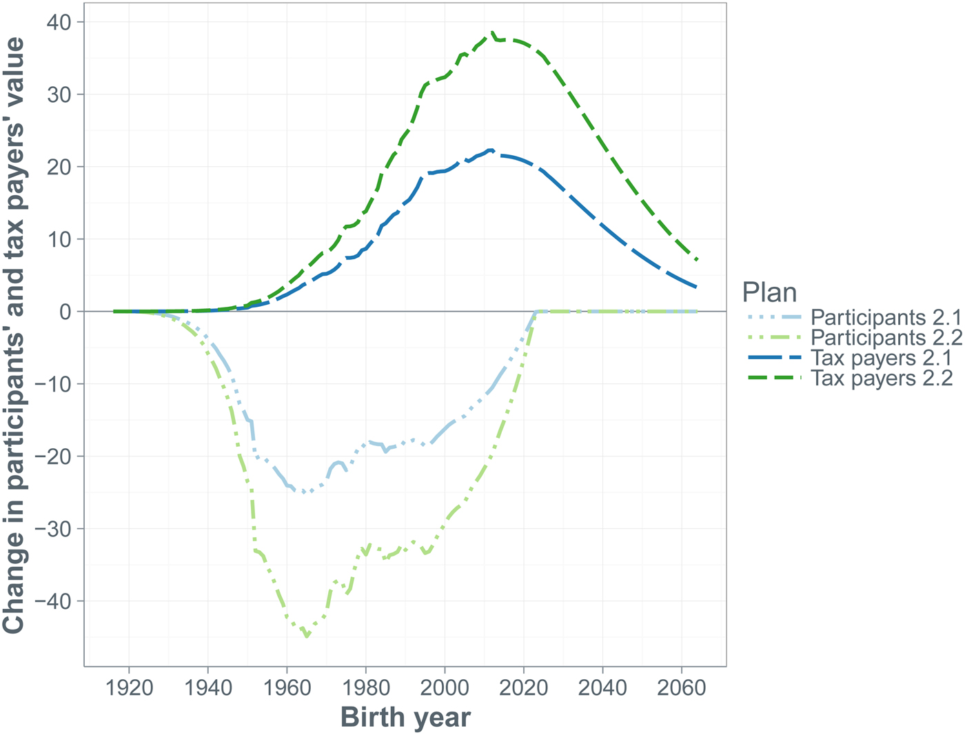
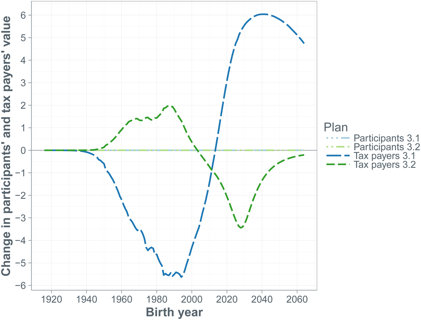
A doubling of the contribution rate by the participants affects their net benefit from the pension contract. The cohorts that have not yet entered the labor force at the start of the simulation horizon experience a value loss equal to more than half the fund's initial assets, while the value loss of the older participants equals one-third of the fund's initial assets. The benefit to both old and young tax payers exceeds 40% of the fund's initial assets. The overall shift from participants to tax payers is about 2.5 trillion dollars. Reducing benefits by cutting indexation can be quite effective too. Halving the indexation to CPI inflation shifts over 1 trillion from participants to tax payers, while making indexation conditional on the funding ratio shifts more than 2 trillion dollars from the former to the latter group. Changes in the pension fund's investment portfolio do not affect the participants’ values, but cause value shifts among cohorts of tax payers. An increase in the riskiness of the portfolio benefits the future tax payers at the expense of the current tax payers, because there is a higher chance of fund's assets being depleted and, consequently, the sponsor having to pay support payments in the short run.
The remainder of this paper is structured as follows. Section 2 relates it to the relevant literature. Section 3 provides a description of the model, discussing the calculation of the pension fund's benefits, contributions and liabilities. Sections 4 and 5, respectively, describe our economic scenario generator and the valuation of the cash flows following from the pension contract. Sections 6 and 7 summarize the data (sources) and the benchmark settings, respectively, while Section 8 presents the various alternative pension plans we will consider. Section 9 discusses the simulation results for the classic ALM and the value-based ALM. It also considers some variations on the benchmark setting. Finally, Section 10 concludes the main text of this paper. All technical details have been relegated to the Appendices, which are not for publication, but will be available online.Footnote 1
2 Relationship with the literature
A recent overview by Munnell et al. (Reference Munnell, Aubry, Hurwitz and Medenica2013) illustrates the urgency of the financial condition of many US state pension funds. For a sample of 109 state plans and 17 locally-administered plans, the paper estimates the aggregate funding ratio (i.e., the ratio of assets over liabilities) for 2012 at 73%. Almost a quarter of the plans have a funding ratio below 60%, while only a small fraction of 6% have a funding ratio above 100%. The funding ratios are calculated on the basis of standards that prescribe that assets are reported on an actuarially-smoothed basis, while the discount rate for the liabilities is typically set at around 8%, reflecting the expected long-term investment return on the fund's assets.Footnote 2 These standards have been criticized by economists (Bader and Gold, Reference Bader and Gold2003; Novy-Marx and Rauh, Reference Novy-Marx and Rauh2009), who claim that the future streams of benefit payments should be discounted at a rate reflecting their riskiness. As the state pension benefits are protected under most state laws, these payments can be seen as guaranteed and so this would plead for discounting them against the risk-free interest rate. In fact, Brown and Pennacchi (Reference Brown and Pennacchi2015) argue that for calculating a pension plan's funding ratio, liabilities should always be discounted against the default-free term structure, no matter what is the actual default risk of the plan. Doing so would lead to a severe fall in the already-low average funding ratios of the state plans. In fact, a precise assessment of the riskiness of state pension promises likely remains elusive for the foreseeable future. For example, the recent default of the city of Detroit on its obligations may be an instructive case of whether pensions should be seen as a contractual obligation that cannot be diminished or impaired, or whether the holders of pension rights should be treated like other creditors, so that benefit cuts cannot be ruled out. Indeed, a US bankruptcy judge declared in December 2013 that legally pensions can be cut (Bomey and Priddle, Reference Bomey and Priddle2013).
The value-based ALM approach that we apply in this paper to US state pension funds has its roots in the pioneering papers of Sharpe (Reference Sharpe1976) and Sharpe and Treynor (Reference Sharpe and Treynor1977) in utilizing derivative pricing to value contingent claims within pension funds. More recent applications of derivative pricing to pension plans are, among others, Blake (Reference Blake1998), Exley et al. (Reference Exley, Mehta and Smith1997), Chapman et al. (Reference Chapman, Gordon and Speed2001), Ponds (Reference Ponds2003), Bader and Gold (Reference Bader and Gold2007), Hoevenaars and Ponds (Reference Hoevenaars and Ponds2008) and Ponds and Lekniute (Reference Ponds and Lekniute2011). Our paper is closest in spirit to Biggs (Reference Biggs2010), which also employs an option-based approach to value the market price of pension liabilities of US state pension plans. However, it does not address reform plans and the associated redistribution effects. Value-based ALM has also been employed in the Dutch discussion on the redesign of the second-pillar pension funds offering DB plans. In particular, the CPB Netherlands Bureau for Economic Policy Analysis (2012) applies it to investigate the generational fairness of various pension reform plans, while Platanakis and Sutcliffe (Reference Platanakis and Sutcliffe2015) apply it to quantify the redistribution associated with the 2011 reform of the UK pension plan for universities (USS).
Our paper is complementary to related contributions studying the degree of underfunding of US state pension plans, the causes of the underfunding and the measures that could be taken to solve plan deficits. Novy-Marx and Rauh (Reference Novy-Marx and Rauh2011) conduct a careful analysis of the value of the pension promises made by US state pension funds under different assumptions about the riskiness of state pension plans and their seniority relative to state debt in the case of default. Several papers explore the extent of underfunding and the question what should be the appropriate target for the funding ratio (compare D'Arcy et al., Reference D'Arcy, Dulebohn and Oh1999; Lucas and Zeldes, Reference Lucas and Zeldes2009; Bohn, Reference Bohn2011). Brown et al. (Reference Brown, Clark and Rauh2011) argue that adequate funding requires 100% funding of the liabilities.
Regarding the causes of the underfunding of state pension plans some papers point at the implications of what may be called the ‘accounting game’. The accountability horizon of politicians and public sector union leaders is much shorter than the horizon over which pension promises have to be met by adequate funding. Hence, union leaders and politicians tend to downplay the long-term costs of pension promises in favor of higher short-term wages and benefits (Mitchel and Smith, Reference Mitchel and Smith1994; Schieber, Reference Schieber2011), as well as higher state spending in the short run. Shnitser (Reference Shnitser2013) stresses the role of the institutional design of pension plans in explaining the large variation in funding discipline. Institutional rules facilitating transparency and pre-commitment to expert-based financial and actuarial advice, in particular, appear to be conducive to mitigating underfunding and limiting the shift of costs to future tax payers. Kelley (Reference Kelley2014) and Elder and Wagner (Reference Elder and Wagner2014) apply a public choice perspective to explaining underfunding issues.
Essentially, the literature has explored three broad directions of solutions to the underfunding problem: higher contributions, lower benefits and higher investment returns. Novy-Marx and Rauh (Reference Novy-Marx and Rauh2014b) explore by how much contributions need to be raised to reach full funding in 30 years time. They compute a necessary increase of the order of 2.5 times the prevailing contribution level. The option of reducing benefits has long been seen as virtually impossible, as in many states public pensions are interpreted as hard contractual obligations, protected by civil law and state constitutions (Monahan, Reference Monahan2012). However, several states have already enacted benefit cuts and other measures to scale back the generosity of pensions. Further, as documented by Munnell et al. (Reference Munnell, Aubry and Cafarelli2014a), in response to the economic and financial crisis, many public plan sponsors have reduced or eliminated cost-of-living-adjustments (COLAs) in one way or the other. Munnell et al. (Reference Munnell, Aubry and Cafarelli2014a) report that between 2010 and 2013 this has been done by 17 states and conclude that benefits are no longer as secure as they were perceived to be before the financial crisis. Novy-Marx and Rauh (Reference Novy-Marx and Rauh2014a) explore performance-linked indexation rules comparable with the one in the Wisconsin Retirement System or the conditional indexation rule in the Netherlands (Ponds and van Riel, Reference Ponds and van Riel2009; Beetsma and Bucciol, Reference Beetsma and Bucciol2010, Reference Beetsma and Bucciol2011a, Reference Beetsma and Bucciolb). Shnitser (Reference Shnitser2013) stresses that simply scaling back generosity or imposing higher contribution rates will not be enough. She claims that foremost the institutional design has to be reframed to practices and rules that have proven to be successful in promoting funding discipline. A third route proposed to solve funding deficits is to raise expected investment returns. This option is already being exploited by US state pension funds, as many of them have high portfolio shares in equity, substantially higher than of pension funds outside the USA (OECD, 2011; Andonov et al., Reference Andonov, Bauer and Cremers2013). However, finance-based papers (Black, Reference Black1989; Peskin, Reference Peskin2001; Bader and Gold, Reference Bader and Gold2003; Lucas and Zeldes, Reference Lucas and Zeldes2009; Pennacchi and Rastad, Reference Pennacchi and Rastad2011) recommend that the strategic asset allocation should be set in line with the perspective of the tax payers as the party bearing the residual risk, which suggests to limit mismatch risk between the funds’ assets and the market value of their liabilities. This may imply no equity investment at all when one aims at full protection of accrued benefits in the short run. Lucas and Zeldes (Reference Lucas and Zeldes2009), employing a long-term perspective, suggest that the optimal portfolio should include some equity holdings as future pension liabilities are related to future wage growth and this growth is to some extent correlated with the equity returns.
3 The model
This section briefly sketches the model. The full details of the model are found in Appendix A. It first describes the demography, then the wage developments and, finally, the pension fund. The participant population of the pension fund consists of individuals of ages 25–99 years. Individuals enter the fund at the age of 25 and remain with the fund for the rest of their life. We distinguish between males and females and apply projections of survival probabilities to calculate the size of these cohorts in the future. The survival probabilities are deterministic, hence there is no longevity risk. Crucial for the calculation of the pension liabilities are the wage developments. We assume a uniform wage level within each cohort, while over one's life the wage level follows a certain career profile that is constant over time (i.e., the relative wage between two cohorts of specific ages is constant over time). Because we do not have gender-specific age-wage profiles, we set the wage levels of males and females equal. The economy-wide wage growth rate is stochastic and will be modelled as explained in Section 4 below.
State pension funds can differ in many respects from each other. Some of the differences are parametric, such as the value of the discount rate to be applied when calculating the liabilities, while other differences are more fundamental. We model a pension fund based on the most common features across the entire population of pension funds available to us from the Public Plans Database of the Center for Retirement Research at Boston College (2015). In doing so, we try to stay as close as possible to the actual practice of GASB accounting employed by pension funds, and use their most common actuarial assumptions to calculate their financial health in actuarial terms, which is the basis for their instrument settings (contributions, indexation and benefits). However, our simulations of the fund over time, and the valuation of the cash flows, will be based on an economic scenario set and a term structure constructed from actual and survey projections of economic and financial data.
3.1 The calculation of the actuarial assets and liabilities
As inputs for policy decisions, we need to calculate the actuarial assets
 $A_t^{act} $
and actuarial liabilities
$A_t^{act} $
and actuarial liabilities
 $L_t^{act} $
to the participants of the fund. These consist of the retired and the workers. Compared with the market value of the assets, the dynamics of the actuarial assets are smoothed, because each period they change only by expected investment income plus a fraction of the difference between realized and expected investment income. The actuarial liabilities are calculated as the present value of the future benefit payments to all current fund participants, taking into account the survival probabilities, and based on the actuarial assumptions typically used by pension funds. The actuarial liabilities should be distinguished from what we will term the economic liabilities, the projected benefits based on the economic developments expected by the market participants and discounted against a proper market interest rate. The economic liabilities will be discussed in more detail below.
$L_t^{act} $
to the participants of the fund. These consist of the retired and the workers. Compared with the market value of the assets, the dynamics of the actuarial assets are smoothed, because each period they change only by expected investment income plus a fraction of the difference between realized and expected investment income. The actuarial liabilities are calculated as the present value of the future benefit payments to all current fund participants, taking into account the survival probabilities, and based on the actuarial assumptions typically used by pension funds. The actuarial liabilities should be distinguished from what we will term the economic liabilities, the projected benefits based on the economic developments expected by the market participants and discounted against a proper market interest rate. The economic liabilities will be discussed in more detail below.
To calculate the actuarial liabilities, see Munnell et al. (Reference Munnell, Haverstick, Sass and Aubry2008b), we need to calculate the projected future benefits of both the retirees and the workers. The projected future benefits equal the current pension rights adjusted for the actuarially projected future COLAs,Footnote 3 intended to protect the retirees’ living standards and calculated on the basis of the fund's own future inflation projection. The current pay-out to a retiree equals their current pension rights, which equals their pension rights at the moment of retirement compounded by the realized COLA since retirement. In turn, pension rights at retirement are the product of the annual accrual rate, the number of years in the workforce and the average over the latest (usually 1–5 years) wages earned by the individual (Munnell et al., Reference Munnell, Aubry, Hurwitz and Quinby2012).
Thus, we need to distinguish the actuarial projection of the COLA and the realized COLA. The latter covers a certain share of realized inflation and is often capped at a predetermined level (Center for Retirement Research at Boston College, 2015). Hence, under our baseline plan and most alternative plans we model the realized COLA as
 $$COLA_t = \max \left[ {\min \left( {\xi \cdot cpi_t,cap} \right),0} \right]$$
where cpi t stands for actual consumer-price inflation in period t, ξ is the fraction that is compensated and cap is the maximum indexation rate. Here, both cpi and cap are expressed as a fraction of unity. The minimum indexation rate is bounded from below at zero, hence benefit payments are prevented from declining in nominal terms. In reality, ξ is often below one. However, in order to avoid an arbitrary parametrization, under our baseline pension plan we will set ξ = 1, while we will consider an alternative plan in which ξ is below one.
In contrast to the retirees, active participants are expected to continue working and, hence, accrue additional years of service. Therefore, there are various ways in which the liabilities associated with the worker's current pension rights can be recognized. Under the Accrued Benefit Obligation (ABO) method, only the pension rights accrued up to now are taken into account, while future wage rises are not taken into account. The Projected Benefit Obligation (PBO) method also takes into account the effect of actuarially projected salary increases on the rights accrued up to now. Finally, the Projected Value of Benefits (PVB) method in addition takes into account the rights that the employees will acquire in the future if they continue working in their current job until retirement. As a result, a cohort that has just entered the labor force already has a stake in the fund's liabilities, as opposed to the ABO or PBO method. For people of working age PVB liabilities would normally exceed PBO liabilities, which, in turn would exceed ABO liabilities. However, all three measures converge for a given individual at the moment of retirement.
The PVB method is of particular relevance here since state civil service jobs are relatively secure. We use the PVB method to calculate our liability measures and the associated pension contributions. The calculations are done under the assumption that individuals spend their full career as fund participants. We make this assumption, because the Public Pensions Database has no information on the entry and exit likelihoods at different ages at the individual fund level or at the aggregate level. Given the upward-sloping age-wage profiles, ignoring entry at later age biases all the liability measures downward, while ignoring job exits that take place before retirement produces an upward bias in our PBO and PVB measures, because the projected salary increases of the quitters would drop out of these measures. In view of the absence of the appropriate data, we have chosen to ignore entries later in working life and premature exits, rather than making arbitrary assumptions about the age distribution of the people entering and leaving the fund.
3.2 The funding ratio
The evaluation of a pension fund's financial health and its policies, including indexation decisions, is usually based on a funding ratio that is calculated on the basis of the fund's actuarial assumptions. We refer to this funding ratio as the policy funding ratio
 $(FR_t^P )$
, defined as the ratio of the fund's actuarial assets and actuarial liabilities:
$(FR_t^P )$
, defined as the ratio of the fund's actuarial assets and actuarial liabilities:
 $$FR_t^P = \displaystyle{{A_t^{act}} \over {L_t^{act}}}. $$
However, the policy funding ratio often gives an overly optimistic picture of the financial health of the pension fund, in particular due to the use of an unrealistically high discount rate for the calculation of the actuarial liabilities. Therefore, we also calculate an economic funding ratio
 $(FR_t^E )$
defined as the ratio of the market value of the assets A
t
and the economic liabilities L
t
:
$(FR_t^E )$
defined as the ratio of the market value of the assets A
t
and the economic liabilities L
t
:
 $$FR_t^E = \displaystyle{{A_t} \over {L_t}}.$$
The economic liabilities are computed by discounting against the (default-free) nominal term structure the projected future benefits based on the expected price and nominal wage developments implied by our model of the dynamics of the state variables, conditional their values in period t (see Section 4 below).
Brown and Pennacchi (Reference Brown and Pennacchi2015) provide a number of arguments for using the default-free nominal term structure for DB pension plans if the funding ratio is intended to measure the fund's financial health. First, the funding ratio thus calculated is independent of the investment portfolio, in contrast to when the liabilities are calculated on the basis of the expected investment return. Second, the funding ratio calculated in this way immediately shows how much more a plan sponsor needs to contribute in the case of underfunding (or would receive back in the case of overfunding) for an insurance company to take over the pension obligations and guarantee the DB payments. Note that the floor and the cap on the indexation rate prevent accumulated entitlements from fully keeping up with inflation. Appropriate account of the floor would shift the term structure for the discounting down, while the opposite is the case when appropriate account is taken of the cap. However, incorporating the effects of the floor and the cap in a fully consistent way is so complicated that we decide to apply the nominal term structure without any further adjustments.
3.3 Benefits and contributions
The total amount of benefits B t paid out by the fund is the sum over all retirement ages of the number of retired at each age times the current pension rights at that age. The total contribution rate c t is total contributions C t divided by the aggregate wage sum. We have that
 $$\eqalign{c_t = & c_t^{NC} + c_t^{Amort} + c_t^{SS} \cr = & c_t^{act} + c_t^{SS},} $$
where
 $c_t^{NC} $
,
$c_t^{NC} $
,
 $c_t^{Amort} $
, and
$c_t^{Amort} $
, and
 $c_t^{SS} $
are the so-called normal cost payment, the (actual) amortization payment and the sponsor support payments, respectively, all as fractions of the aggregate wage sum. Finally, we refer to
$c_t^{SS} $
are the so-called normal cost payment, the (actual) amortization payment and the sponsor support payments, respectively, all as fractions of the aggregate wage sum. Finally, we refer to
 $c_t^{act} = c_t^{NC} + c_t^{Amort} $
as the actuarial contribution rate.
$c_t^{act} = c_t^{NC} + c_t^{Amort} $
as the actuarial contribution rate.
The normal cost equals the value of the additional pension rights earned in a given year. The amortization payment is based on the so-called unfunded actuarial accrued liability (UAAL), which, in turn, is the difference between the actuarial accrued liability,
 $L_{accr,t}^{act} $
, and the actuarial value of the assets, i.e.,
$L_{accr,t}^{act} $
, and the actuarial value of the assets, i.e.,
 $UAAL_t = L_{accr,t}^{act} - A_t^{act} $
. We assume a smoothing period of u years for the amortization of the UAAL
t
. The amortization payment cannot be negative. If there is a funding surplus, i.e., UAAL
t
< 0, the actuarial contribution is kept at the normal cost covering contribution
$UAAL_t = L_{accr,t}^{act} - A_t^{act} $
. We assume a smoothing period of u years for the amortization of the UAAL
t
. The amortization payment cannot be negative. If there is a funding surplus, i.e., UAAL
t
< 0, the actuarial contribution is kept at the normal cost covering contribution
 $c_t^{NC} $
, hence
$c_t^{NC} $
, hence
 $c_t^{Amort} = 0$
. Munnell et al. (Reference Munnell, Haverstick, Aubry and Golub-Sass2008a) show that in only about half of all the pension plans the required amortization contribution is paid. In our simulations we thus allow for only a fraction of the required amortization payment to be actually paid.
$c_t^{Amort} = 0$
. Munnell et al. (Reference Munnell, Haverstick, Aubry and Golub-Sass2008a) show that in only about half of all the pension plans the required amortization contribution is paid. In our simulations we thus allow for only a fraction of the required amortization payment to be actually paid.
Forecasting the development of a pension fund over a long horizon implies that there exist scenarios in which the fund's assets get depleted.Footnote
4
We assume that, whenever the fund's assets A
t
become insufficient to finance the net cash outflow B
t
− C
t
, the employer, i.e., the tax payer,Footnote
5
provides sponsor support SS
t
. Hence,
 $SS_t = (B_t - C_t) - A_t$
, if this is positive. Otherwise, SS
t
= 0. Once the sponsor support becomes positive, the fund effectively continues to be run on a pay-as-you-go basis. Both the policy and economic funding ratios remain at zero from that moment onwards.
$SS_t = (B_t - C_t) - A_t$
, if this is positive. Otherwise, SS
t
= 0. Once the sponsor support becomes positive, the fund effectively continues to be run on a pay-as-you-go basis. Both the policy and economic funding ratios remain at zero from that moment onwards.
The actuarial contribution rate can be split into a contribution rate
 $c_t^{PP} $
paid by the plan participant and a contribution rate
$c_t^{PP} $
paid by the plan participant and a contribution rate
 $c_t^{TP} $
paid by the tax payer (as employer):
$c_t^{TP} $
paid by the tax payer (as employer):
 $$c_t^{act} = c_t^{PP} + c_t^{TP}. $$
Typically, as we will also assume in our simulations, the contribution rate paid by the worker is fixed, i.e.,
 $c_t^{PP} $
is constant, while the tax payer as employer pays the remainder.
$c_t^{PP} $
is constant, while the tax payer as employer pays the remainder.
4 The economic scenario generator
We estimate a quarterly vector autoregression (VAR) model on historical data for the USA and use this model to generate a set of economic scenarios.Footnote 6 It is generally not known which scenario will occur in reality. Hence, we evaluate the performance of an object of interest under all the scenarios that we generate. For our purposes, there is no need for a very refined model specification. Hence, we simply use a first-order VAR model linking the state vector in quarter q + 1 to that in quarter q:
 $$X_{q + 1} = \left[ {\matrix{ {y_{q + 1}} \cr {xs_{q + 1}} \cr {cpi_{q + 1}} \cr {w_{q + 1}} \cr}} \right] = \alpha + \Gamma X_q + \varepsilon _{q + 1},$$
where y
q+1 is the short-term quarterly interest rate, xs
q+1 is the excess return on stocks, cpi
q+1 is consumer price inflation and w
q+1 is real wage growth. The first two variables are calculated by taking the natural logarithm of the gross rate. The latter two variables are calculated as changes in the logarithm of the relevant index. The error terms ε
q+1 are independently and identically distributed and follow a multivariate normal distribution with mean zero and variance-covariance matrix Σ. Further,
 $\alpha = (I - \Gamma )\mu $
, where I denotes the identity matrix and μ is the unconditional mean of the vector X
q
for all q. The estimates
$\alpha = (I - \Gamma )\mu $
, where I denotes the identity matrix and μ is the unconditional mean of the vector X
q
for all q. The estimates
 $\hat \alpha $
and
$\hat \alpha $
and
 $\hat \Gamma $
of α and Γ, respectively, are obtained by estimating equation (6) using OLS. We obtain
$\hat \Gamma $
of α and Γ, respectively, are obtained by estimating equation (6) using OLS. We obtain
 $\hat \Sigma $
as the variance-covariance estimate of the error terms.Footnote
7
Given
$\hat \Sigma $
as the variance-covariance estimate of the error terms.Footnote
7
Given
 $\hat \Gamma $
and
$\hat \Gamma $
and
 $\hat \alpha $
, the estimate of μ is:
$\hat \alpha $
, the estimate of μ is:
 $$\hat \mu = (I - \hat \Gamma )^{ - 1}\hat \alpha. $$
The parameter estimates associated with (6) are used to price the cash flows implied by the pension arrangement.
5 Valuation
A pension plan can be seen as a financial contract. If we perceive this contract as a combination of contingent claims, we can value the pension deal using the derivative pricing techniques of risk-neutral valuation introduced by Black and Scholes (Reference Black and Scholes1973). Below, we explain how we calculate the value of the pension contract for all pension fund stakeholders, i.e., for the individual cohorts of participants and the individual cohorts of tax payers. Aggregating over the individual cohorts we obtain the contract value for all participants as a group and all the tax payers as a group.
To value the contract we use the scenarios for the underlying state vector produced by our scenario generator. The scenarios are generated at the quarterly frequency. We draw both real-world (‘P world’) scenarios for the classic ALM model and risk-neutral (‘Q world’) scenarios for the value-based ALM model. Under the classic ALM we generate paths for the state vector drawing shocks from a zero-mean normal density function, while under value-based ALM we generate these paths using risk-neutral sampling, which effectively amounts to a negative shift in the means of the components of the original shock vector.
The path for the state vector thus gives us a path for the stock returns. Also, for each quarter into the simulation, we determine the term structure using an affine model based on the state variables (e.g., see Dai and Singleton, Reference Dai and Singleton2000; Ang and Piazzesi, Reference Ang and Piazzesi2003; Ang et al., Reference Ang, Bekaert and Wei2008; Le et al., Reference Le, Singleton and Dai2010). This allows us to calculate the return on the fixed income part of the fund's portfolio, so that we now have the return on the entire fund portfolio. Using the path of the state vector generated under the risk-neutral sampling, as well as the returns on the fund's portfolio based on this same path of the state vector, allows us to generate the annual cash flows associated with the pension contract under the value-based ALM. These are then discounted against the risk-free rate of interest. Appendix B shows the details of the pricing of the cash flows and Appendix C of the transformation to the risk-neutral scenarios needed to calculate the value of the pension contract to the various stakeholders.
We aim at valuing the pension contract to the different stakeholders of the fund. Therefore, we will calculate the value of the net benefits to each cohort of fund participants and each cohort of tax payers. We will value the cash flows over a horizon of T years. Recall that the scenarios are simulated at the quarterly frequency, while the cash flows materialize at the annual frequency.
The value
 $V_0^{PP,a} $
of the pension contract to plan participants of the cohort aged a at t = 0 is:
$V_0^{PP,a} $
of the pension contract to plan participants of the cohort aged a at t = 0 is:
 $$V_0^{PP,a} = {\rm E}_0^Q \left[ {\sum\limits_{t = 1}^T \left( {\prod\limits_{q = 1}^{4t - 2} {(Y_q)}^{ - 1}} \right)NB_t^a + \left( {\prod\limits_{q = 1}^{4T - 2} {(Y_q)}^{ - 1}} \right)\tilde L_T^a} \right],$$
where
 ${\rm E}_0^Q $
is the risk-neutral expectation under the Q measure of the cash flows discounted against the quarterly gross risk-free rate Y
q
, obtained through the simulation of the state vector, and q denotes the quarter.
${\rm E}_0^Q $
is the risk-neutral expectation under the Q measure of the cash flows discounted against the quarterly gross risk-free rate Y
q
, obtained through the simulation of the state vector, and q denotes the quarter.
 $NB_t^a $
is the net benefit of the cohort aged a in period t, which for workers is their contribution and for pensioners is the pension benefit they receive. Hence,
$NB_t^a $
is the net benefit of the cohort aged a in period t, which for workers is their contribution and for pensioners is the pension benefit they receive. Hence,
 $NB_t^a $
is negative for workers and positive for retirees. Because
$NB_t^a $
is negative for workers and positive for retirees. Because
 $NB_t^a $
occurs in the middle of time period t, it is discounted only for half of year t. Further,
$NB_t^a $
occurs in the middle of time period t, it is discounted only for half of year t. Further,
 $\tilde L_T^a $
is the final value of the economic liabilities to the cohort of age a. Since the working participants accrue pension entitlements in exchange for their contributions, we add the discounted final value of the economic liabilities to the discounted value of the net benefits to arrive at the value of the contract for each cohort. Unlike benefits and contributions, the outstanding pension entitlements at the end of the simulation period are not actual cash flows that materialize during the simulation. Rather, they form an estimate of the outstanding pension promises that have been given in exchange for contributions paid earlier. To sum up, the contract value to a cohort is defined as the present value of the benefits they receive, minus present value of their contributions, plus the present value of the pension entitlements accrued at the end of the simulation horizon in exchange for the contributions made earlier. The contract value to all participants is the sum of the contract values for each cohort participating in the fund during the evaluation horizon, i.e.,
$\tilde L_T^a $
is the final value of the economic liabilities to the cohort of age a. Since the working participants accrue pension entitlements in exchange for their contributions, we add the discounted final value of the economic liabilities to the discounted value of the net benefits to arrive at the value of the contract for each cohort. Unlike benefits and contributions, the outstanding pension entitlements at the end of the simulation period are not actual cash flows that materialize during the simulation. Rather, they form an estimate of the outstanding pension promises that have been given in exchange for contributions paid earlier. To sum up, the contract value to a cohort is defined as the present value of the benefits they receive, minus present value of their contributions, plus the present value of the pension entitlements accrued at the end of the simulation horizon in exchange for the contributions made earlier. The contract value to all participants is the sum of the contract values for each cohort participating in the fund during the evaluation horizon, i.e.,
 $V_0^{PP} = \sum\nolimits_a V_0^{PP,a} $
.
$V_0^{PP} = \sum\nolimits_a V_0^{PP,a} $
.
The value of the contract to the tax payer cohort of age a in period 0 is:
 $$V_0^{TP,a} = - {\rm E}_0^Q \left[ {\sum\limits_{t = 1}^T \left( {\prod\limits_{q = 1}^{4t - 2} {(Y_q)}^{ - 1}} \right)\left( {C_t^{TP,a} + SS_t^a} \right) - V_0^{R,a}} \right],$$
where
 $C_t^{TP,a} $
is the tax-payers’ contribution in dollars, i.e., the normal cost plus the actual amortization payment minus the contribution by the employees, and
$C_t^{TP,a} $
is the tax-payers’ contribution in dollars, i.e., the normal cost plus the actual amortization payment minus the contribution by the employees, and
 $SS_t^a $
the sponsor support. The contract value to the total population of tax payers is
$SS_t^a $
the sponsor support. The contract value to the total population of tax payers is
 $V_0^{TP} = \sum\nolimits_a V_0^{TP,a} $
. The final term in (9) is the part of the so-called residual value of the pension fund absorbed by the cohort of age a. The residual value
$V_0^{TP} = \sum\nolimits_a V_0^{TP,a} $
. The final term in (9) is the part of the so-called residual value of the pension fund absorbed by the cohort of age a. The residual value
 $V_0^R = {\rm E}_0^Q \left[ {\prod\nolimits_{q = 1}^{4T - 2} {(Y_q)}^{ - 1}(A_T - {\tilde L}_T)} \right]$
is the difference between the present value of the assets remaining at the end of the evaluation horizon and the aggregate of the final values of the economic liabilities. Therefore, it is what is left over in present value terms for the tax payers at the end of the simulation horizon after redeeming their obligations to the fund participants still alive at that moment. Since the contributions associated with these accrued liabilities by the tax payers as employers have already been made, we can view the residual value as the amount of resources that the tax payers alive at the end of the horizon would still need to provide to (if the residual is negative) or receive from (if the residual is positive) the fund participants. We therefore distribute the residual value over all cohorts of tax payers alive at the end of the horizon.
$V_0^R = {\rm E}_0^Q \left[ {\prod\nolimits_{q = 1}^{4T - 2} {(Y_q)}^{ - 1}(A_T - {\tilde L}_T)} \right]$
is the difference between the present value of the assets remaining at the end of the evaluation horizon and the aggregate of the final values of the economic liabilities. Therefore, it is what is left over in present value terms for the tax payers at the end of the simulation horizon after redeeming their obligations to the fund participants still alive at that moment. Since the contributions associated with these accrued liabilities by the tax payers as employers have already been made, we can view the residual value as the amount of resources that the tax payers alive at the end of the horizon would still need to provide to (if the residual is negative) or receive from (if the residual is positive) the fund participants. We therefore distribute the residual value over all cohorts of tax payers alive at the end of the horizon.
The cohort-specific plan participant values are immediately available, as participants always contribute a certain part of their cohort-specific salary and receive cohort-specific benefit payments. Determining the cohort-specific tax payer values is not completely straightforward. The aggregate cash flows in a year from all the tax payers together are immediately available. However, calculating the contract values for the individual cohorts of tax payers aged a in period 0 requires an assumption about the allocation of the aggregate cash flows across the cohorts of tax payers. We assume that the demographic structure of the tax payer population and the age-wage profiles of the tax payers are identical to those of the participant population. The cash flows assigned to a specific tax payer cohort are then proportional to the share of this specific cohort in aggregate income. For tax payers of working age, the relative contribution of each cohort is fixed over time through the age-wage profile, because the latter is constant over time. The relative contribution of a cohort of retired tax payers is proportional to the average income of the participant cohort (i.e., the retirement benefit) relative to average aggregate income, where average income is the average over all scenarios in a specific year under the baseline plan. When allocating the residual value, we assume that it is absorbed by the different cohorts of tax payers alive at the end of the horizon in proportion to the present value of their projected remaining lifetime income.
6 The data
All our data are for the USA. Our dataset comprises macroeconomic data, data from financial markets, data on state pension funds and demographic data. The economic scenario generator described earlier is based on historical data spanning the first quarter of 1990 up to and including the second quarter of 2015.
We use historical time series of the short interest rate, stock returns, price inflation and wage inflation. We obtain the real wage growth rate by adjusting the nominal wage growth rate by the growth rate in the nominal price index. The short interest rate is the 3-month treasury rate series and is obtained from the Board of Governors of the Federal Reserve System (2015). For the stock returns we use the NYSE/Amex/Nasdaq value-weighted return with dividends, which is available from the Center for Research in Security Prices (2015). For price inflation we use the CPI index provided by the Bureau of Labor Statistics (2015). Finally, wage inflation is obtained from the compensation of employees, wages and salary accruals and is retrieved from the US. Bureau of Economic Analysis (2015). These data are all quarterly or of higher frequency and transformed into quarterly data. The US treasury nominal yield curve for maturities from 1 to 10 years is retrieved from the Federal Reserve Board (2015). We obtain the treasury real yield curve rates for maturities 5, 7 and 10 from the US Department of the Treasury (2015). However, they are only available starting from 2003. Finally, we obtain pension plan data from the Public Plans Database of the Center for Retirement Research at Boston College (2015).
As far as the demography is concerned, we use the National Population Estimates for 2010 by single year of age and sex provided by the United States Census Bureau (2014). Further, we use the survival rates derived from the Cohort Life Tables for the Social Security Area by Year of Birth and Sex provided by the US Social Security Administration (2014) These life tables are available for birth years with 10 years intervals. Therefore, we linearly interpolate the survival rates for the birth years in between the ones directly available.
7 Benchmark settings for our US state plan
We set the benchmark simulation horizon to 75 years, which is a commonly-used horizon for pension policy evaluation in the USA and which allows us to take into account a large number of cohorts that enter the fund after the start of the evaluation horizon. Hence, we evaluate the pension contract for cohorts born up to 50 years from now, in effect assuming that for cohorts born later contributions will be set such that their net contract value is zero. Extending the simulation horizon, we observe that the present values of both the end-of-the-horizon assets and economic liabilities fall and, hence, become less relevant relative to the present value of the benefits paid out over the horizon. In Subsection 9.3.3, we show that extending the horizon to 100 years has no qualitative and only limited quantitative effect on our results.
The demographic structure of our fund at the start t = 0 of the simulation horizon is assumed to be identical to that of the US population in 2010. Hence, the relative sizes of the cohorts are equal to those for the USA in 2010. We set the population of our pension fund at t = 0 equal to the aggregate number of participants in 2012 of all the state plans covered by the data from the Center for Retirement Research at Boston College (2015). As a result, our pension fund initially has approximately 26 million participants. While these data do not include all the US public pension plans, they do include a very substantial share of the US public sector workers at the sub-national level. Hence, the magnitude of the net burden on the tax payers that we will expose below provides a good indication of the seriousness of the public sector pension underfunding problem for the USA, although it may only be a lower bound to the problem. This is not only because a number of public plans have not been included in our dataset – and a priori there is little reason to assume that these plans are healthier than those that are part of our dataset –, but also because the lion's share of the cost to the tax payers will be in the most underfunded, riskiest plans, since tax payer guarantees are increasing and convex in risk.Footnote 8 Obviously, when financial pressure accumulates, the subnational authorities will start shifting new participants into DC plans. However, we aim at assessing the underfunding problem under current plans and plausible alternatives, so here we ignore other potential policy reactions to the problem.
The fund's demography over the simulation horizon evolves as follows. Throughout the simulation horizon new cohorts aged 25 enter the labor market and become participants of the pension fund. Hence, for the first 25 years of the simulation horizon we determine the sizes of the 25-year old cohort by taking the sizes of the cohorts younger than 25 in the US population initially and projecting the size of each such cohort when it reaches the age of 25 by using the officially projected (gender-specific) survival probabilities. The number of new entrants for the remaining 50 years of a simulation run is calculated by extending over time the trend in the size of the 25-year old cohort, i.e., by calculating the average annual growth rate of the 25-year old cohort over the first 25 years of the simulation horizon and taking this as the annual growth rate for the next 50 years. At the start of the simulation there are about 280 thousand 25-year old males and about 270 thousand 25-year old females entering the fund. During the first 25 years the number of new 25-year olds decreases on average by 0.34% per year. Extrapolating this trend over the next 50 years yields roughly 210 thousand new male entrants and 200 thousand new female entrants in the final simulation year.
Our simulations are based on the most common characteristics of the US state pension plans. Its liabilities are computed by using the entry age normal (EAN) actuarial method for liability recognition and are based on the following assumptions. Individuals retire at the age of 65. Hence, a full career means that they work for 40 years. The career (age-wage) profile is obtained from Bucciol (Reference Bucciol2012). Because the shape of this profile does not change over time, the wage earned at a given age increases each year with the common wage growth rate in the economy. The t = 0 average wage rate is set such that the fund's initial liabilities L 0 are equal to 3900 billion dollars, which is the aggregate amount of liabilities in 2012 over all pension funds in the Public Plans Database of the Center for Retirement Research at Boston College (2015).Footnote 9 The benefit factor, or accrual rate, is 2% for each additional year of service, while the earnings base for the retirement benefit is the average of the final 3 years of pay during the career. During retirement there is full indexation for consumer price inflation when inflation is non-negative, while indexation is set at zero when inflation is negative.
The actuarial assumptions by our pension fund are based on the median assumptions used by the funds in the Public Plans Database of the Center for Retirement Research at Boston College (2015) in 2012 (the most recent year for which there is a full sample available). As a result, projected benefits are heightened up with a projected nominal salary increase of 3.75% for each working year and a projected annual rate of price inflation of 3.16% for each year in retirement, while the future retirement benefits are discounted at a fixed rate of 7.75% a year. We assume the initial accrued pension rights,
 $B_0^a $
, to have been fully indexed up to time t = 0.
$B_0^a $
, to have been fully indexed up to time t = 0.
Contributions to the fund are calculated as follows. The annually required contribution is set to the normal cost plus the required amortization payment, which we assumed to be fixed at zero in the case of a fund surplus (one-sided policy). The normal cost is calculated as a percentage of the projected career salary based on the EAN actuarial method. The amortization payment is determined by spreading the unfunded actuarial accrued liability UAAL in equal annual payments over the next 30 years, with a moving 30-years window. Hence, we use the so-called open amortization period. Employees pay a fixed 6% contribution of their salary, while the tax payer as employer pays the remainder of the required contribution.
Our sample data show that in 2012, assuming that the normal cost is paid in full, the actual amortization payment is on average just slightly more than half of the required amortization payment. Because of the lack of potentially more representative data we assume that the actual contribution is set to 100% of the normal cost, plus 50% of the required amortization payment. However, because our estimate of the share of required amortization paid varies substantially across plans and because of the importance of this parameter to the funding situation of the plan, we will also examine variations on the baseline plan in which less or more of the required amortization payment is paid in a year.
We set the initial actuarial funding ratio FR 0 equal to 71%, which is the median funding ratio of the pension funds in our database in 2012. Based on FR 0 and the initial liabilities, which are thus both matched to our data, we obtain the initial actuarial assets of the fund:
 $$A_0^{act} = FR_0 \cdot L_0.$$
The actuarial funding position of the pension fund in the subsequent periods is calculated as the ratio of the actuarial assets and liabilities.Footnote 10
We assume that under the baseline plan the fund invests 50% of its assets in fixed income (with an average annual return of 4.7%) and the other 50% in risky assets (with an average annual return of 5.5%). This implies an average annual return on the fund's portfolio of 5.1%. We thus abstract from investments in assets other than these two classes.Footnote 11
8 The alternative plans
We consider a number of variations on the baseline plan, which we refer to as Plan 0, to explore what various policy changes imply for the contract values of the different stakeholders. This can give us leads about the effectiveness of different measures in reducing the likelihood that the pension fund's assets get depleted and, hence, in reducing reliance on the support from the tax payers.
We consider three groups of measures, which we summarize in Table 1. The first set of measures, Plans 1.1–1.4, addresses the contribution rate. Plans 1.1 and 1.2 vary the fraction of the required amortization payment actually paid, Plan 1.3 shortens the period over which the amortization payment is spread, while Plan 1.4 doubles the contribution payment by the participants from 6% to 12% of their salary, but leaves the total contribution rate and, hence, the fund's financial health unchanged.
Table 1. Summary of the alternative plans
The second set of alternatives addresses the degree of indexation. Under all plans, including the baseline plan, there is a 0% floor on indexation. Plan 2.1 halves indexation when CPI inflation is positive. Under Plan 2.2, if CPI inflation is positive, then indexation to CPI inflation is conditional on the level of the policy funding ratio FR
P
. Specifically, if cpi ≥ 0 and FR
P
<0.5, indexation is 0, while if cpi ≥ 0 and FR
P
≥ 0.5, it equals
 $(2FR^P - 1)cpi$
. Therefore, if CPI inflation is positive, indexation is zero for funding ratios below one half, while it increases linearly with the funding ratio for funding ratios of at least one half. Hence, a funding ratio above unity implies more than full indexation. This way of providing conditional indexation is closely related to the way most Dutch pension funds index their pension rights – see Ponds and van Riel (Reference Ponds and van Riel2009) and Beetsma and Bucciol (Reference Beetsma and Bucciol2011b).
$(2FR^P - 1)cpi$
. Therefore, if CPI inflation is positive, indexation is zero for funding ratios below one half, while it increases linearly with the funding ratio for funding ratios of at least one half. Hence, a funding ratio above unity implies more than full indexation. This way of providing conditional indexation is closely related to the way most Dutch pension funds index their pension rights – see Ponds and van Riel (Reference Ponds and van Riel2009) and Beetsma and Bucciol (Reference Beetsma and Bucciol2011b).
We continue to set contributions on the basis of the normal cost that was calculated under the assumption of full indexation. We do this in order to see the isolated effect of a change in indexation. Otherwise, the comparison with the baseline plan would be contaminated by a fall of the normal cost when indexation is reduced, which through lower contributions would in turn dampen the beneficial effect of less indexation on the fund's financial health.
The third group of measures concerns the composition of the fund's asset portfolio, which we vary from zero to 100% stocks.
9 Results
Appendix E reports the quarterly frequency estimates of
 $\hat \mu $
and
$\hat \mu $
and
 $\hat \Sigma $
of the VAR model (6) over the period 1990Q1–2015Q2. It also computes the correlation matrix of the vector of state variables. Not surprisingly, the shocks to the excess stock return are most volatile. Also not surprisingly, the correlation between the short-interest rate and CPI inflation is positive, while the correlation between CPI inflation and real wage growth is negative. If the nominal wage is sticky, then positive shocks to inflation have a negative effect on real wage growth. Finally, real wage growth is positively correlated with the excess stock returns, which is, for example, in line with the prediction of the standard neoclassical macroeconomic model driven by total factor productivity shocks.
$\hat \Sigma $
of the VAR model (6) over the period 1990Q1–2015Q2. It also computes the correlation matrix of the vector of state variables. Not surprisingly, the shocks to the excess stock return are most volatile. Also not surprisingly, the correlation between the short-interest rate and CPI inflation is positive, while the correlation between CPI inflation and real wage growth is negative. If the nominal wage is sticky, then positive shocks to inflation have a negative effect on real wage growth. Finally, real wage growth is positively correlated with the excess stock returns, which is, for example, in line with the prediction of the standard neoclassical macroeconomic model driven by total factor productivity shocks.
The economic outlook nowadays differs substantially from the average economic situation over our sample period 1990Q1–2015Q2. Because historically observed values are unlikely to provide the best estimate of expected future values, in the simulation of our benchmark scenario set we replace the estimated vector of means
 $\hat \mu $
with the medians of the 10-year-ahead forecasts taken from the SPF in 2015Q1 as provided by the Federal Reserve Bank of Philadelphia (2015). Hence, we impute an annual average of 5.5% for the stock returns, 2.7% for the short interest rate and 2.1% for consumer price inflation. The SPF does not report projections for real wage growth. Hence, to impute SPF projections for the entire
$\hat \mu $
with the medians of the 10-year-ahead forecasts taken from the SPF in 2015Q1 as provided by the Federal Reserve Bank of Philadelphia (2015). Hence, we impute an annual average of 5.5% for the stock returns, 2.7% for the short interest rate and 2.1% for consumer price inflation. The SPF does not report projections for real wage growth. Hence, to impute SPF projections for the entire
 $\hat \mu $
-vector, we replace the average real wage growth estimate with the SPF projection of productivity growth, which is 1.7%. Actually, this gives a scenario set that is very similar to the one we get if we would not replace the average real wage growth estimate. We properly transform these annual values into quarterly values. We continue to work with the original variance-covariance matrix
$\hat \mu $
-vector, we replace the average real wage growth estimate with the SPF projection of productivity growth, which is 1.7%. Actually, this gives a scenario set that is very similar to the one we get if we would not replace the average real wage growth estimate. We properly transform these annual values into quarterly values. We continue to work with the original variance-covariance matrix
 $\hat \Sigma $
estimated above.
$\hat \Sigma $
estimated above.
As a robustness check on our main findings, in Subsection 9.3 we discuss the results based on a scenario set in which we do not impute the SPF forecasts, but use the original
 $\hat \mu $
-vector estimate for the means of the state variables. Our benchmark results leave the inflation risk premium free to be determined along with the parameters of the yield curve. In Subsection 9.3 we show that the numerical results are close to their benchmark values if we exogenously impose an inflation risk premium at specific values in line with findings elsewhere (see also Grishchenko and Huang, Reference Grishchenko and Huang2012). There, we also show that extending the evaluation horizon to 100 years has no qualitative and only limited quantitative impact on our findings.
$\hat \mu $
-vector estimate for the means of the state variables. Our benchmark results leave the inflation risk premium free to be determined along with the parameters of the yield curve. In Subsection 9.3 we show that the numerical results are close to their benchmark values if we exogenously impose an inflation risk premium at specific values in line with findings elsewhere (see also Grishchenko and Huang, Reference Grishchenko and Huang2012). There, we also show that extending the evaluation horizon to 100 years has no qualitative and only limited quantitative impact on our findings.
The inputs for our calculations come from different years. Because the financial market projections are based on data for the year 2015, in the sequel we assume that the beginning of the evaluation period t = 0 corresponds to the year 2015. Obviously, the implicit assumption is that the funding ratios and demography of the funds have not changed too much over the past couple of years.
9.1 The ‘classic’ ALM benchmark results
This subsection discusses the ‘classic’ (i.e., not applying market-based valuation) ALM simulation results under the baseline plan and the alternative plans. Here, and in the sequel, we simulate the pension fund's performance for a set of 5000 economic scenarios over a horizon of 75 years.
Table 2 reports for the various plans the 5%, 50% and 95% percentiles after 25 years for the total contribution rate c and its components, the normal cost payment c
NC
, the amortization payment c
Amort
and the sponsor support payment c
SS
, all in percentages of the wage sum. For the normal cost payment we present only one column, because the normal cost depends only on the assumptions made by the fund and is therefore constant across scenarios. Table 2 reports the numbers for the policy funding ratio FR
P
, the economic funding ratio FR
E
and the pension result PR after 25 years. The pension result is defined as the ratio of the cumulative granted indexation to the cumulative price inflation, i.e.,
 $PR_t = \prod\nolimits_{\tau = 0}^t (1 + COLA_\tau )/(1 + cpi_\tau )$
. Hence, the lower it is, the larger the deterioration in the purchasing power of the benefits. Table 3 reports all the corresponding numbers after 75 years.
$PR_t = \prod\nolimits_{\tau = 0}^t (1 + COLA_\tau )/(1 + cpi_\tau )$
. Hence, the lower it is, the larger the deterioration in the purchasing power of the benefits. Table 3 reports all the corresponding numbers after 75 years.
Table 2. Classic ALM results under different plans after 25 years

Note: Classic ALM results after 25 years for the 5%, 50% and 95% percentiles of (a) the total contribution rate (c), which is the sum of the normal cost
 $(c^{NC})$
, amortization
$(c^{NC})$
, amortization
 $(c^{Amort})$
, and sponsor support payment
$(c^{Amort})$
, and sponsor support payment
 $(c^{SS})$
, all in percentages of the wage sum, and (b) the policy funding ratio
$(c^{SS})$
, all in percentages of the wage sum, and (b) the policy funding ratio
 $(FR^P)$
, the economic funding ratio
$(FR^P)$
, the economic funding ratio
 $(FR^E)$
, and the pension result (PR) for the baseline Plan 0 and alternative contribution (Plans 1.1–1.3), indexation (Plans 2.1–2.2) and investment (Plans 3.1–3.2) policies. Note that the median values of the components of c do not necessarily add up to the median value of c. The policy funding ratio is defined as actuarial assets over actuarial liabilities, the economic funding ratio as market value of assets over economic liabilities, and the pension result as the ratio of cumulative granted indexation to cumulative price inflation.
$(FR^E)$
, and the pension result (PR) for the baseline Plan 0 and alternative contribution (Plans 1.1–1.3), indexation (Plans 2.1–2.2) and investment (Plans 3.1–3.2) policies. Note that the median values of the components of c do not necessarily add up to the median value of c. The policy funding ratio is defined as actuarial assets over actuarial liabilities, the economic funding ratio as market value of assets over economic liabilities, and the pension result as the ratio of cumulative granted indexation to cumulative price inflation.
Table 3. Classic ALM results under different plans after 75 years

Note: Classic ALM results after 75 years for the 5%, 50%, and 95% percentiles of (a) the total contribution rate (c), which is the sum of the normal cost
 $(c^{NC})$
, amortization
$(c^{NC})$
, amortization
 $(c^{Amort})$
, and sponsor support payment
$(c^{Amort})$
, and sponsor support payment
 $(c^{SS})$
, all in percentages of the wage sum, and (b) the policy funding ratio
$(c^{SS})$
, all in percentages of the wage sum, and (b) the policy funding ratio
 $(FR^P)$
, the economic funding ratio
$(FR^P)$
, the economic funding ratio
 $(FR^E)$
, and the pension result (PR) for the baseline Plan 0 and alternative contribution (Plans 1.1–1.3), indexation (Plans 2.1–2.2) and investment (Plans 3.1–3.2) policies. Note that the median values of the components of c do not necessarily add up to the median value of c. The policy funding ratio is defined as actuarial assets over actuarial liabilities, the economic funding ratio as market value of assets over economic liabilities, and the pension result as the ratio of cumulative granted indexation to cumulative price inflation.
$(FR^E)$
, and the pension result (PR) for the baseline Plan 0 and alternative contribution (Plans 1.1–1.3), indexation (Plans 2.1–2.2) and investment (Plans 3.1–3.2) policies. Note that the median values of the components of c do not necessarily add up to the median value of c. The policy funding ratio is defined as actuarial assets over actuarial liabilities, the economic funding ratio as market value of assets over economic liabilities, and the pension result as the ratio of cumulative granted indexation to cumulative price inflation.
Consider first the results for the baseline Plan 0. The normal cost contribution at t = 0 is 12% and the total contribution is 14%. After 25 years, the respective median values are 12% and 20%, while the median amortization contribution is 8% (note that generally the median total is not the sum of the other two medians, as they likely correspond to different scenarios). The median sponsor support is 0%. After 75 years, the median total contribution has risen to 41%. The median sponsor support contribution is now of the same order of magnitude as the median amortization contribution. After 25 years the median value of the policy funding ratio is only 28%, while after 75 years the median has fallen to zero. After 75 years even the 95th percentile of the policy funding ratio is zero. The economic funding ratio, which provides a more accurate assessment of the fund's financial health, is even lower than the policy funding ratio as long as the latter is positive. Once the assets have been depleted and consequently the policy funding ratio has fallen to zero, the fund is effectively run on a pay-as-you-go basis, with benefits on a period-by-period basis financed through the various payments by the employees and the tax payers. The gradual run-down of the fund's assets can no longer be used as a cushion against the drastic increase in the total contribution rate. The bleak long-run financial outlook for the fund is not surprising in view of the fact that the expected return on its asset portfolio falls short of its discount rate, while only 50% of the required amortization costs is paid when the fund's financial health is poor (and, given its rolling window of 30 years, the required amortization itself adjusts only slowly to a financial deterioration of the fund). The pension result exceeds 100% after 75 years at the three reported percentiles, because full indexation is always granted when inflation is positive and zero in the case of deflation. Table 4 reports the probability that all assets are fully depleted within the 75-year simulation horizon. This probability is 97% for the baseline plan, while, conditional on a full depletion taking place, the median year in which this happens is 41 years from the start of the simulation.
Table 4. Likelihood of full depletion of assets
Note: The first column reports the probability that the fund's assets are fully depleted within the 75-year simulation horizon. The following columns show the quantiles for the distribution of the years of full depletion, conditional on scenarios in which depletion takes place within the simulation horizon. As an example, under the baseline Plan 0, conditional on depletion taking place, 27 is the maximum number of years in which this happens in less than 5% of the cases. Therefore, the quantile is attained at 28.
It is important to realize that extreme outcomes, like a full depletion of the fund's assets, are unlikely to occur in reality, because before such an extreme outcome materializes, policymakers would have undertaken some action to avoid it. However, we want to see what the consequences of adhering to the baseline Plan 0 are. The high likelihood that this leads to full asset depletion is precisely the reason why we explore whether specific alternatives to the baseline plan can mitigate the deterioration of the long-run financial health of the fund, as well as the rise in tax payer contributions. When no amortization payments are made (Plan 1.1), initially the total contribution rate is equal to the normal cost. However, this leads to an even more dramatic expected deterioration of the policy funding ratio than under the baseline plan. Already after 25 years the median policy funding ratio is only 7%, while the economic funding ratio is only 4%. Again, after 75 years the funding ratios at all percentiles we consider are zero. This eventually leads to the same total contribution rate as under the baseline plan, but this time via a different route, namely, the sponsor support instead of the amortization payments. A shift to 100% amortization under Plan 1.2 provides slightly better protection of the fund's financial health, leaving the median policy funding ratio after 75 years at 11%. The shift from 0% to 100% amortization contribution implies a shift away from sponsor support contribution, because it reduces the likelihood of complete asset depletion. In this case the median total contribution rate after 75 years is 37%, while the median amortization contribution is 24% and the median sponsor support contribution is zero. A shift to an amortization period of 10 years has a similar effect. The plans 1.1–1.3 are sorted in terms of how well the plan's underfunding reflects in the amortization payments. The stricter the amortization policy, the higher the amortization payments (hence also total contributions) are in the short term, but the lower the total contributions in the longer term. The numbers for the funding ratios, total contributions and amortization contributions under Plan 1.4 are identical to those under the baseline plan. Hence, we do not separately report them in the tables. However, the component of the normal cost paid by the participants has been doubled.
The second set of alternative measures introduces changes in the indexation rate. Plan 2.1 always yields lower indexation when CPI inflation is positive, implying that in the not too distant future the funding ratio holds up better than under the baseline plan (the median policy funding ratio after 25 years is now 35% versus 28% under the baseline plan). This is even more so the case under conditional indexation (Plan 2.2), because indexation becomes particularly low when the policy funding ratio is low. However, after 75 years, both the median policy funding ratio and median economic funding ratio are zero under both alternatives. Not surprisingly, the alternative indexation policies affect the pension result negatively. Its median value after 75 years drops to less than 50% when indexation is halved and it drops to only a quarter under conditional indexation. Reduced generosity in terms of indexation favors the tax payers who benefit from a reduction in amortization contributions and, in particular, from a reduction in sponsor support contribution.
Our third set of measures looks at changes in the pension fund's asset portfolio. Not surprisingly, because of the increased riskiness, a policy of investing 100% of the asset portfolio in stocks, Plan 3.1, produces an increase in the spread of the funding ratio compared to the baseline plan after 25 years. The 5% percentile of the policy funding ratio is zero and the median is 23%. However, the 95th percentile is 148%. Nevertheless, in the long run, after 75 years, the median policy funding ratio is still zero, because the overoptimistic actuarial projection of the portfolio return exceeds the actual average return on the portfolio. There is some chance that stocks do on average extremely well over the full horizon and, hence, that the burden on the tax payers turns out to be low. Indeed the 5th percentile of the amortization contribution is 5% and of the sponsor support contribution is 0%. However, the medians of these components are the same as under the baseline plan. A switch to 100% bonds compresses the spread in the policy funding ratio in the shorter run, so that even its 5th percentile is still positive after 25 years. However, in the long run even the 95th percentile has fallen to zero. The quantiles of the amortization and sponsor support contributions are very much in line with the corresponding quantiles under the baseline plan.
Overall, it can be concluded that under many of the settings studied here the chances of the pension fund ending the 75-year horizon with positive assets are low. The only exception is the alternative of a 10-year amortization period. An important factor is the high actuarial discount rate used by the fund, which exceeds the lower average return on the investment portfolio and thus leads to inadequate contributions to keep the fund financially healthy. With such a discrepancy between the actuarial discount rate and the average performance of the asset portfolio even a substantially less generous indexation policy may not be enough to prevent the fund from running out of assets. The other important factor concerns the tax payers’ discipline in paying the normal cost and the amortization payments fully. Once the amortization is paid fully, or even better, the amortization period is shortened, the funding situation may improve substantially.
9.2 The value-based ALM benchmark results
In the previous subsection we have used a classic ALM analysis to explore to what extent alternatives to the baseline plan can reduce the likelihood that the pension fund's assets get depleted. Value-based ALM is useful to assess changes in the market value of the pension contract to its various stakeholders when shifting from the baseline plan to another plan.
We evaluate at t = 0 the baseline plan, as well as alternatives to the baseline. In value terms, reforms are zero-sum games across the fund's stakeholders (plan participants and tax payers):
 $$\Delta V_0^{PP} + \Delta V_0^{TP} = 0,$$
where
 $V_0^s $
is the contract value for stakeholder s ( = PP or TP) under the baseline plan and
$V_0^s $
is the contract value for stakeholder s ( = PP or TP) under the baseline plan and
 $\Delta V_0^s \equiv \tilde V_0^s - V_0^s $
is the change in value from the baseline plan, where
$\Delta V_0^s \equiv \tilde V_0^s - V_0^s $
is the change in value from the baseline plan, where
 $\tilde V_0^s $
is the value under the alternative plan. The fund's initial assets do not appear in this expression, as we start with the same value of initial assets under all plans, hence the change in its value is always zero. We are also interested in the relative change ΔRV
0 in the values of the various stakeholders, computed as:
$\tilde V_0^s $
is the value under the alternative plan. The fund's initial assets do not appear in this expression, as we start with the same value of initial assets under all plans, hence the change in its value is always zero. We are also interested in the relative change ΔRV
0 in the values of the various stakeholders, computed as:
 $$\Delta RV_0^s = \displaystyle{{\tilde V_0^s - V_0^s} \over {A_0}} \times 100\%. $$
We express the relative change as a fraction of a common denominator, which we choose to be the value of the initial assets A 0. This way we obtain an impression of the importance of the relative change compared with the scale A 0 on which the fund operates.
We report contract values for the entire group of participants, the entire group of tax payers, individual cohorts of participants and individual cohorts of tax payers.
9.2.1 The baseline plan
Figure 1 shows for the baseline Plan 0 the value of the contract
 $V_0^{PP,a} $
and
$V_0^{PP,a} $
and
 $V_0^{TP,a} $
in billions of dollars for the various cohorts of fund participants and tax payers, respectively. The youngest generation is the one to be born in 50 years from t = 0 (it has age −50 at t = 0, i.e., the year 2015), whereas the oldest is 99 years old at the start of the simulation period. Here, t = 0 is the year 2015. The figure gives an impression of the order of magnitude of the aggregate amounts at stake for the various cohorts of stakeholders in the state civil service pension funds. In present value terms, under the baseline plan over the 75-year simulation horizon, the value of the aggregate net benefit plus the final economic liabilities to all participant cohorts is approximately 14 trillion dollars, while the value of the aggregate contribution over all tax payer cohorts minus the value of the final assets is approximately 11 trillion dollars.Footnote
12
The difference equals the fund's initial assets. These are sizable numbers and, as indicated earlier, they likely form a lower bound on the actual amount of redistribution from tax payers to fund participants. We see that the value of the contract is positive for all participant cohorts. This is mostly due to the fact that participants pay only a part of total contribution. Also, for the older cohorts that are in the fund initially, the contributions are sunk, while their benefits are still ahead of them. For the current elderly the contract value starts falling steeply with age, as the amount of remaining future benefits to be received is shrinking with age.
$V_0^{TP,a} $
in billions of dollars for the various cohorts of fund participants and tax payers, respectively. The youngest generation is the one to be born in 50 years from t = 0 (it has age −50 at t = 0, i.e., the year 2015), whereas the oldest is 99 years old at the start of the simulation period. Here, t = 0 is the year 2015. The figure gives an impression of the order of magnitude of the aggregate amounts at stake for the various cohorts of stakeholders in the state civil service pension funds. In present value terms, under the baseline plan over the 75-year simulation horizon, the value of the aggregate net benefit plus the final economic liabilities to all participant cohorts is approximately 14 trillion dollars, while the value of the aggregate contribution over all tax payer cohorts minus the value of the final assets is approximately 11 trillion dollars.Footnote
12
The difference equals the fund's initial assets. These are sizable numbers and, as indicated earlier, they likely form a lower bound on the actual amount of redistribution from tax payers to fund participants. We see that the value of the contract is positive for all participant cohorts. This is mostly due to the fact that participants pay only a part of total contribution. Also, for the older cohorts that are in the fund initially, the contributions are sunk, while their benefits are still ahead of them. For the current elderly the contract value starts falling steeply with age, as the amount of remaining future benefits to be received is shrinking with age.
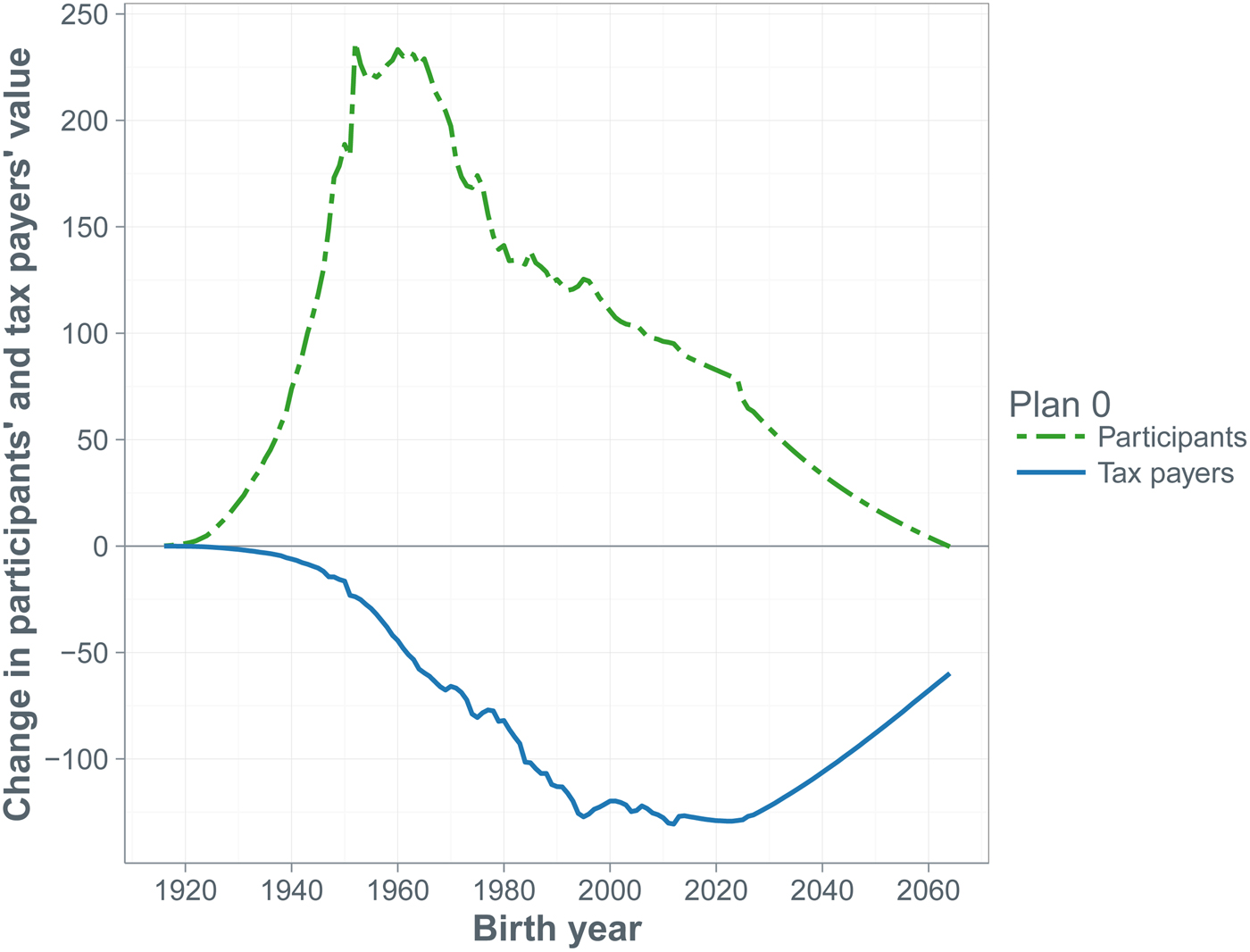
Figure 1. (Colour online) Stakeholder contract values under the baseline plan. Note: participants’ and tax payers’ contract values by age cohort under the baseline Plan 0, in billions of dollars.
For the cohorts of age 25 and younger at t = 0, the positive contract value needs more explanation, because in a completely actuarially-neutral system, those who have not yet been contributing would experience zero value from their pension contract: the value of their future benefits must be offset by the value of their future contributions. However, this value is only zero for the cohort born at t = 50 (i.e., the year 2065), because over the evaluation horizon this cohort will pay zero contributions and thus build up zero rights. For future generations that will be born before t = 50, the value of the benefits they will receive over the evaluation horizon plus the value of the accrued rights at the end of the evaluation period exceeds the value of the contributions to be made during the evaluation period. This net benefit must be financed out of the fund's initial assets or through contributions from the tax payers. From the figure we observe that the value of the plan
 $V_0^{TP,a} $
is negative for all the cohorts of tax payers.
$V_0^{TP,a} $
is negative for all the cohorts of tax payers.
9.2.2 Outcomes of the alternative plans
We report changes in dollar values and in relative values for groups of cohorts of participants and tax payers resulting from alternative plans. The results are reported in Table 5(a) (for changes in dollar values) and Table 5(b) (for changes in relative values) for two groups of participants and two groups of tax payers. Negative relative values denote a deterioration compared with the baseline plan for the particular stakeholders under consideration. The group of the ‘young’ (superscript Y) comprises all the cohorts younger than 25 or yet unborn at t = 0, while the group of the ‘old’ (superscript O) comprises all the cohorts of age 25 or older at t = 0, hence all the active or retired participants at t = 0. As explained above, theoretically, for each alternative plan, the sum of value changes must be zero, i.e.,
 $\Delta V_0^{PP,Y} + \Delta V_0^{PP,O} + \Delta V_0^{TP,Y} +$
 $ \Delta V_0^{TP,O} = 0$
. However, due to numerical inaccuracies small deviations from zero may be possible.
$ \Delta V_0^{TP,O} = 0$
. However, due to numerical inaccuracies small deviations from zero may be possible.
Table 5. Effects of plan changes on stakeholders
Note: The table reports the effects of switching from baseline Plan 0 to Plans 1.1–3.2 on future plan participants
 $(\Delta V_0^{PP,Y}, \,\Delta RV_0^{PP,Y} )$
, current plan participants
$(\Delta V_0^{PP,Y}, \,\Delta RV_0^{PP,Y} )$
, current plan participants
 $(\Delta V_0^{PP,O}, \,\Delta RV_0^{PP,O} )$
, future tax payers
$(\Delta V_0^{PP,O}, \,\Delta RV_0^{PP,O} )$
, future tax payers
 $(\Delta V_0^{TP,Y}, \,\Delta RV_0^{TP,Y} )$
, and current tax payers
$(\Delta V_0^{TP,Y}, \,\Delta RV_0^{TP,Y} )$
, and current tax payers
 $(\Delta V_0^{TP,O}, \,\Delta RV_0^{TP,O} )$
. Panel (a) reports the value of the baseline plan and the change in value of switching from the baseline to an alternative plan in billions of dollars. Panel (b) reports relative changes as percentages of the fund's initial assets A
0. Negative numbers imply a deterioration of the value for that stakeholder.
$(\Delta V_0^{TP,O}, \,\Delta RV_0^{TP,O} )$
. Panel (a) reports the value of the baseline plan and the change in value of switching from the baseline to an alternative plan in billions of dollars. Panel (b) reports relative changes as percentages of the fund's initial assets A
0. Negative numbers imply a deterioration of the value for that stakeholder.
Under Plans 1.1–1.3 neither the contributions made by the plan participants nor the indexation rules are changed, so
 $\Delta V_0^{PP,Y} = \Delta V_0^{PP,O} = 0$
. A reduction in the amortization payment (Plan 1.1) benefits current tax payers, because they see their amortization contribution rate fall. However, it affects future cohorts of tax payers negatively, as they have to cover the deficit with sponsor support payments once assets get completely depleted, which now happens earlier. An increase in the amortization payment, Plan 1.2, has the opposite effect and benefits the young tax payers, while the old tax payers lose out. A similar conclusion holds for a shortening of the period over which the amortization takes place, Plan 1.3. A doubling of the contribution rate by the participants, Plan 1.4, reduces the total contribution paid by the tax payers and, thus, shifts value from both groups of participants to the tax payers. The aggregate value shift exceeds 2.5 trillion dollars. In percentage terms the older participants lose one-third of the contract value, while the younger participants lose more than half of their value.
$\Delta V_0^{PP,Y} = \Delta V_0^{PP,O} = 0$
. A reduction in the amortization payment (Plan 1.1) benefits current tax payers, because they see their amortization contribution rate fall. However, it affects future cohorts of tax payers negatively, as they have to cover the deficit with sponsor support payments once assets get completely depleted, which now happens earlier. An increase in the amortization payment, Plan 1.2, has the opposite effect and benefits the young tax payers, while the old tax payers lose out. A similar conclusion holds for a shortening of the period over which the amortization takes place, Plan 1.3. A doubling of the contribution rate by the participants, Plan 1.4, reduces the total contribution paid by the tax payers and, thus, shifts value from both groups of participants to the tax payers. The aggregate value shift exceeds 2.5 trillion dollars. In percentage terms the older participants lose one-third of the contract value, while the younger participants lose more than half of their value.
Changes in indexation policy shift value between the participants and the tax payers. Halving indexation, Plan 2.1, lowers the plan value to the participants and raises the plan value to the tax payers, who have to pay smaller amortization and sponsor support contributions. The aggregate value loss to the participants is about 1.4 trillion dollars, or 14% of initial fund assets for the younger participants and one-third of initial fund assets for the older participants. Especially the young tax payers benefit, the reason being that the reduction in indexation reduces the tax payer support most when the fund's assets are depleted or almost depleted. Conditional indexation, Plan 2.2, produces qualitatively similar, but quantitatively even larger value shifts across the stakeholders. In fact, the loss of the older participants is 60% of initial fund assets, while that of the younger participants is more than a quarter of initial fund assets. Older tax payers gain 15% of initial fund assets, while young tax payers even gain 72% of initial fund assets.
Our third set of changes concerns changes in the composition of the asset portfolio of the pension fund. In all of the previous plans the asset mix was kept constant at 50% fixed income and 50% risky assets. When the portfolio allocation is the same across the plans, the total amount of risk remains unchanged, but it is shifted among stakeholders due to policy changes, like changes in the contribution or indexation rules. Changing the asset mix changes the riskiness of the pension fund's asset portfolio itself. Since neither indexation policy, nor the participant contribution rules have changed, the fund participants are unaffected by changes in the composition of the fund's asset portfolio. However, there are shifts in value across the tax payers. A shift to 100% stocks (Plan 3.1) affects older tax payers negatively, but younger tax payers positively. Older tax payers suffer, because in the shorter run the increased riskiness of the fund raises the chance that the fund completely runs out of assets. This makes it more likely that the older taxpayers need to support the pension benefits on a pay-as-you-go basis. For the younger tax payers, this would be the overwhelmingly likely prospect in any case. An increase in riskiness of the asset portfolio raises the likelihood of positive assets in the longer run, thereby lowering the chance that the current younger taxpayers have to pay the benefits on a pay-as-you-go basis later in working life. So the states of the world with earlier fund depletion under the riskier strategy do not hurt the younger taxpayers, while they benefit from the possible states of the world where these riskier asset strategies perform well. In the case of de-risking (Plan 3.2), we observe the opposite effects. Obviously, these and other policy changes that redistribute across cohorts of tax payers could in principle be undone through an appropriate combination of public debt and tax policies.
Figures 2–4 depict the value consequences of contract changes for all individual cohorts of participants and tax payers. In line with the numbers reported in the above tables, we see indeed that moving from the baseline plan to Plan 1.1 with zero amortization (see Figure 2) the older tax payers are better off, as part of the contribution burden is shifted to the future, while younger cohorts of tax payers have to contribute more to make up for the losses of the fund. Contributions are shifted from amortization to sponsor support. However, in contrast to amortization, sponsor support only needs to be provided when the fund's assets are depleted, which generally takes place some decades after the start of the evaluation period. Moving to 100% amortization, Plan 1.2, works in the opposite direction and, hence, reduces the value for the older tax payers, but benefits the younger tax payers. The same is the case when amortization is speeded up (Plan 1.3), which has even stronger negative effects on the older tax payers and stronger positive effects on the younger tax payers. Finally, a doubling of the contribution by the workers affects all the workers’ values negatively and all the tax payers’ values positively. The retired participants are unaffected.
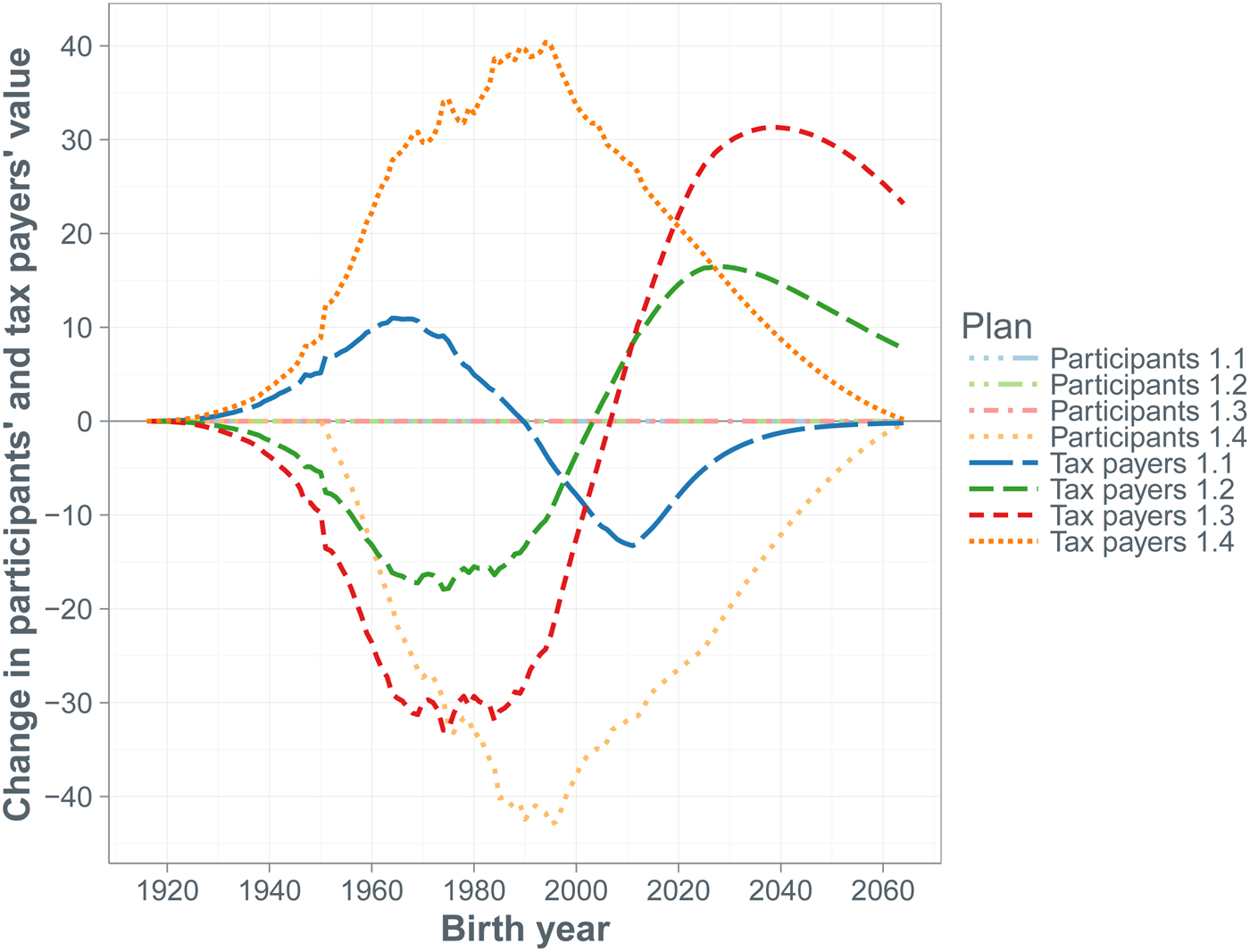
Figure 2. (Colour online) Changes in stakeholder contract values from contribution reforms. Note: this figure depicts by age cohort the change in the stakeholder contract value (in billions of dollars) when policy is changed from the baseline Plan 0 to plans with no amortization payment (Plan 1.1), full amortization payment (Plan 1.2), 10 years amortization smoothing (Plan 1.3) and a doubling of the contribution rate by employees (Plan 1.4).

Figure 3. (Colour online) Changes in stakeholder contract values from indexation reforms. Note: this figure depicts by age cohort the change in the stakeholder contract value (in billions of dollars) when policy is changed from the baseline Plan 0 to plans with half CPI indexation (Plan 2.1) and conditional indexation (Plan 2.2).

Figure 4. (Colour online) Changes in stakeholder contract values from changes in the fund's asset portfolio composition. Note: this figure depicts by age cohort the change in the stakeholder contract value (in billions of dollars) when policy is changed from the baseline Plan 0 to plans with 100% risky assets (Plan 3.1) and 100% fixed income assets (Plan 3.2).
Not surprisingly, a shift from full indexation to compensation of only half of the CPI, i.e., a shift from Plan 0 to Plan 2.1 (see Figure 3), lowers the contract value to all participant cohorts currently alive and born up to 10 years from the start of the simulation horizon. All cohorts that enter the fund later see no change in value, because they will not receive any pension benefit over the simulation horizon, while their contributions are unchanged. Recall that under all the plans that we consider, including Plan 2.1, the calculation of the contributions and the economic liabilities at the end of the simulation horizon, based on the expected price and nominal wage developments implied by our estimated VAR model, is done as if indexation is full. Only the actual indexation in retirement is adjusted. Hence, cohorts that do not reach retirement within the simulation horizon are not affected by this plan. All cohorts of tax payers benefit from the shift to Plan 2.1. Similarly, since indexation tends on average to be lower under conditional indexation, also Plan 2.2 affects the value for all participants that are already retired or reach retirement during the simulation horizon negatively, while all tax payer cohorts are better off. Again, those participant cohorts born more than 10 years into the future are unaffected. Quantitatively, the effects on all the cohorts of tax payers and participants, except those that will not reach retirement during the simulation horizon, are larger than under Plan 2.1. This is the result of tendency for the funding ratio to sharply deteriorate over the simulation horizon, implying that there will be very little or no indexation when indexation is made conditional. Finally, looking at an increase in risk of the pension fund's portfolio (see Figure 4), we observe that all the participating cohorts are unaffected, while young tax payers benefit from a more risky portfolio and old tax payers lose, as explained above. The opposite is the case when the portfolio is made less risky.
9.3 Robustness analysis
9.3.1 More optimistic assumptions about the asset returns
There is substantial uncertainty surrounding the expected returns on financial variables. Hence, in reality there is a good chance that the realisations of our state vector deviate quite substantially from the benchmark expected values underlying our scenario set. For our benchmark scenario set, we found that it is highly likely that the fund's assets will be depleted over the simulation horizon. In this subsection we show that the likelihood of a severe asset deterioration of the fund will still be high even under substantially more optimistic assumptions about the asset returns. In particular, in this subsection we base the means of the state vector in our scenario set on the originally-estimated
 $\hat \mu $
vector, i.e., we do not adjust the means according to the SPF forecast. In particular, investment returns will be higher under this alternative setting: the average annual portfolio return will be 7.7%, based on 50% in fixed income with an average annual return of 4% and 50% in risky assets with an average annual return of 11.3%.
$\hat \mu $
vector, i.e., we do not adjust the means according to the SPF forecast. In particular, investment returns will be higher under this alternative setting: the average annual portfolio return will be 7.7%, based on 50% in fixed income with an average annual return of 4% and 50% in risky assets with an average annual return of 11.3%.
Because only the means of state vector are changed, the scenario set under risk-neutral sampling is unchanged and, hence, the value-based ALM results are unaffected. Therefore, we do not discuss them further and we focus here on the changes in the classic ALM results. To save space, we report only the quantiles of the relevant variables after 75 years – see Table 6. Because of the higher portfolio returns, assets tend to fall at a slower pace and, hence, amortization and sponsor support contributions tend to be smaller. As a result, the median total contribution rate of 21% under Plan 0 is much lower than the median of 41% under the benchmark scenario set. The same holds for the other plans, except for Plan 1.1 (0% amortization paid) and Plan 3.2 (0% stocks). Except for these two plans, the median amortization contribution rate has become much lower. This is also the case for the median sponsor support contribution rate under the baseline Plan 0, Plan 1.4 (doubling of the participants’ contribution rate), Plans 2.1 and 2.2 involving reduced indexation and Plan 3.1 involving 100% stocks.
Table 6. Classic ALM results under different plans after 75 years (sensitivity scenario set)
Note: Classic ALM results after 75 years for the 5%, 50%, and 95% percentiles of (a) the total contribution rate (c), which is the sum of the normal cost
 $(c^{NC})$
, amortization
$(c^{NC})$
, amortization
 $(c^{Amort})$
, and sponsor support payment
$(c^{Amort})$
, and sponsor support payment
 $(c^{SS})$
, all in percentages of the wage sum, and (b) the policy funding ratio
$(c^{SS})$
, all in percentages of the wage sum, and (b) the policy funding ratio
 $(FR^P)$
, the economic funding ratio
$(FR^P)$
, the economic funding ratio
 $(FR^E)$
, and the pension result (PR) for the baseline Plan 0 and alternative contribution (Plans 1.1–1.3), indexation (Plans 2.1–2.2) and investment (Plans 3.1–3.2) policies. Note that the median values of the components of c do not necessarily add up to the median value of c. The policy funding ratio is defined as actuarial assets over actuarial liabilities, the economic funding ratio as market value of assets over economic liabilities and the pension result as the ratio of cumulative granted indexation to cumulative price inflation.
$(FR^E)$
, and the pension result (PR) for the baseline Plan 0 and alternative contribution (Plans 1.1–1.3), indexation (Plans 2.1–2.2) and investment (Plans 3.1–3.2) policies. Note that the median values of the components of c do not necessarily add up to the median value of c. The policy funding ratio is defined as actuarial assets over actuarial liabilities, the economic funding ratio as market value of assets over economic liabilities and the pension result as the ratio of cumulative granted indexation to cumulative price inflation.
Turning to the funding ratios, we observe that under the baseline Plan 0 the median policy funding ratio is 37%, which still implies that there is a substantial chance of a severe deterioration of the fund's financial position over our horizon. Extreme outcomes in both directions are possible. At the fifth percentile, the policy funding ratio is 0%, while at the 95th percentile it is close to 900%, which reflects the possibility of stocks doing very well over extended periods of time. Obviously, such extreme funding ratios are very unlikely to materialize, because long before policy adjustments, such as a reduction in contribution rates, would have been implemented. However, we want to report the consequences of consistently sticking to a given plan. Increasing or speeding up amortization (Plans 1.2 and 1.3) or reducing indexation (Plans 2.1 and 2.2) are now much more effective at protecting the policy funding ratio in the longer run. The economic funding ratios are always below the policy funding ratios, reflecting the fact that the latter ones are based on actuarial assumptions that do not reflect the risk-free nature of the benefits. The figures for the pension results do not differ much from those under the benchmark scenario set, which reflects the fact that the lower portfolio returns under the benchmark scenario set are primarily the problem of the tax payer. The exception is Plan 2.2 of conditional indexation, under which also the participant substantially benefits from the higher portfolio returns: the higher policy funding ratio under the alternative scenario set allows for more indexation on average.
Table 7 reports the likelihood and speed of asset depletion over our 75-year horizon. Under the base Plan 0, the likelihood of full depletion has fallen to less than 40%. While this is still substantial, it is much lower than the near-certainty of full depletion under the benchmark scenario set. Increasing or speeding up amortization (Plans 1.2 and 1.3) brings the likelihood of full depletion to zero or nearly zero, while making indexation much less generous (Plans 2.1 and 2.2) substantially lowers the likelihood of full depletion. Conditional on full depletion occurring during the simulation horizon, we observe that it tends to occur later than under the benchmark scenario set. For example, under the baseline Plan 0 the median year in which this occurs rises from 41 to 57 from the start of the simulation.
Table 7. Likelihood of full depletion of assets (sensitivity scenario set)

Note: The first column reports the probability that the fund's assets are fully depleted within the 75-year simulation horizon. The following columns show the quantiles for the distribution of the years of depletion, conditional on scenarios in which depletion takes place within the simulation horizon. As an example, under the baseline Plan 0, conditional on depletion taking place, 35 is the maximum number of years in which this happens in less than 5% of the cases. Therefore, the quantile is attained at 36.
9.3.2 Alternative exogenous inflation risk premia
While our benchmark analysis leaves the inflation risk premium to be determined as part of the parameter optimization procedure, there is little consensus about the size of the inflation risk premium in the literature and, a priori, there is no reason to believe that our estimate is more accurate than estimates reported elsewhere in the literature. Hence, it is important to explore whether our findings are sensitive to the size of the inflation risk premium. Therefore, in this subsection we impose an exogenous inflation risk premium that deviates from the inflation risk premium that was endogenously determined under the benchmark. The annual inflation risk premium that follows endogenously from the optimization equals minus 62 basis points. We consider an inflation risk premium of zero, which may be a natural choice in the absence of any prior knowledge about its size, and one of plus 20 basis points annually. The latter choice is motivated by Brown and Pennacchi (Reference Brown and Pennacchi2015) who find an annual inflation risk premium of 21 basis points over 2004–2014 for the USA. Because their estimate refers to 10-year debt and ours to short-run 3-month debt, the two cases are not entirely comparable. However, the sensitivity of our results to the inflation risk premium seems to be too low for this to be a relevant mismatch.
The numerical results for these variants are reported in Appendix F. We observe that the classic ALM results are close to the original results. The most important consequence of a higher inflation risk premium is that the frequency distribution of the funding ratios tends to shift to the right. The reason is that an increase in the inflation risk premium raises the required return on nominal debt and the resulting increase in the average portfolio return of the fund mitigates the decline in its assets. However, the effect is so marginal that the chance that the fund is out of assets at the end of the evaluation horizon is still overwhelming. As far as the value-based ALM results are concerned, the contract values of the different groups of stakeholders tend to be quite close to, though a bit larger, in absolute size than the original ones. The relative effects also tend to become slightly larger in absolute size, especially for the alternative inflation indexation plans.
9.3.3 Extending the evaluation horizon to 100 years
In our final robustness experiment we extend the evaluation horizon to 100 years. The numerical results of this variant are also reported in Appendix F. Obviously, the frequency distributions of the funding ratios at the end of the horizon shift further to the left, and the chances that the system survives such a long period are close to zero. As regards to the value-based ALM results, we expect no effect on the groups that are alive at the start of the evaluation period: they were all dead at the end of the 75 year horizon, so nothing changes for them. However, as we should expect, the positive (negative) contract value of the young participants (tax payers) increases in size. The reason is that young cohorts benefit over a longer period from the contributions by the tax payers. Hence, the shift in relative values for these groups also increases in absolute magnitude for deviations from the baseline Plan 0.
10 Concluding remarks
This paper has explored the financial and redistributive aspects of a typical US state DB pension fund under unchanged policies. The results confirm what is generally feared, namely that continuing current pension policies leads to the depletion of the fund's assets. Even a substantially more optimistic outlook for financial markets than that under our benchmark parameter setting does not solve the long-run financial sustainability issues of the US state pension sector. In fact, the magnitude of this problem exposed by the current paper may well form a lower bound to its true extent, because our dataset did not include all civil servants’ pension funds. A priori, there is little reason to assume that the funds that have not been included are financially healthier than the funds that were part of our dataset. Hence, a continuation of current pension policies is likely to confront the tax payers with an enormous bill, because in principle they have to guarantee the accumulated entitlements of the funds’ participants. Even rather substantial shifts in the structure of the pension contributions or substantial reductions in inflation indexation are unlikely to resolve the long-run financial issues of the US state pension sector, although they may slow down the deterioration of its financial health somewhat.
The looming financial burden on tax payers and the prospective deterioration of public services may discourage individuals of working age from working in states where the pension funding problems are worst. An outcome with falling spending on public goods and rising taxes merely paid to finance civil servants’ retirement schemes may become politically unsustainable and result in states defaulting on their pension obligations. This could well cause larger value losses to fund participants than those associated with orderly reforms backed by a majority of the population.
The analysis in this paper can be extended into various directions, for example by exploring the consequences of closing the fund to new participants or closing it even for contributions from current participants. Also, by applying our method of value-based ALM, we can study value shifts between tax payers and participants for individual state funds and explore which states face the most urgent need for pension reform.
Supplementary material
The supplementary material for this article can be found at https://doi.org/10.1017/S1474747216000214