Introduction
Through the wall using microwave radar imaging (TWRI) is an emerging field of technology which has attracted many researchers and scientists and also motivated them to put their effort for continuous improvement in the system with the contribution of new techniques and algorithms despite of various challenges like portability of detection, reliability, wall parameter estimation, and also acquisition time. There are several imaging algorithms exist, mentioned in the literature, based on the assumption that wall parameters (thickness and dielectric constant) are accurately known but in real scenario, wrong estimation of these parameters affects focused image [Reference Soldovieri, Prisco and Solimene1–Reference Dehmollaian and Sarabandi4]. Several studies have been conducted to estimate the wall parameters, e.g. its thickness and dielectric constant [Reference Wang, Amin and Zhang5, Reference Ahmad, Amin and Mandapati6] using a radar. The true location of a target has been estimated for unknown wall parameters on the basis of the intersection points of trajectory, which can be obtained by shifting the wall parameters, but, this algorithm is not able to generate the complete focused image behind the wall [Reference Wang, Amin and Zhang5]. The wall parameter estimation on the basis of higher order statistics has been carried out on the assumption that point target is placed at far field from through-the wall imaging (TWI) system, however, it is quite complex and a time-consuming process [Reference Ahmad, Amin and Mandapati6]. Previously, in the TWI system dynamic image has been generated at different focusing times, though, the focused image generated was of good quality and simulation time was less, but, the imaging algorithm included the multilayer Green's function, which seems complex [Reference Li, Zhang and Li7]. The echo-domain-filter-based technique and the image-domain-filter-based technique have been used to estimate the thickness and dielectric constant of an unknown wall and obtained good quality of results for TWI scenario, but, the results are based on only the simulation with the help of the 2-D finite-difference time-domain (FDTD) method [Reference Jin, Chen and Zhou8].
The true location of the object behind the wall and its image formation is the main challenge which is quite dependent upon the wall parameters like its thickness and its dielectric constant. The incorrect knowledge of these parameters leads to dislocation and blurring of the image. There is another major challenge to eliminate the unwanted signals and to eliminate the effect of the wall. For this, complete statistical analyses like singular value decomposition (SVD), principal component analysis (PCA), factor analysis (FA), and independent component analysis (ICA) are required to minimize the clutter [Reference Verma, Gaikwad, Singh and Nigam9].
Therefore, in this work, the nonlinear optimization approach using a genetic algorithm (GA) has been used to estimate wall parameters and obtain the complete focused image of a metal target behind a concrete wall. The current work is organized as follows: “Target arrangements and imaging system” section depicts the experimental arrangement and the operating parameters being used for TWI system designing, whereas, the conventional theory and the technique has been mentioned in “Conventional theory and technique” section. The proposed method and optimization technique is explained in “Proposed technique” section, the results on the basis of the proposed method has been described in “Results and discussion” section, and, eventually, entire work is concluded in “Conclusion” section.
Target arrangements and imaging system
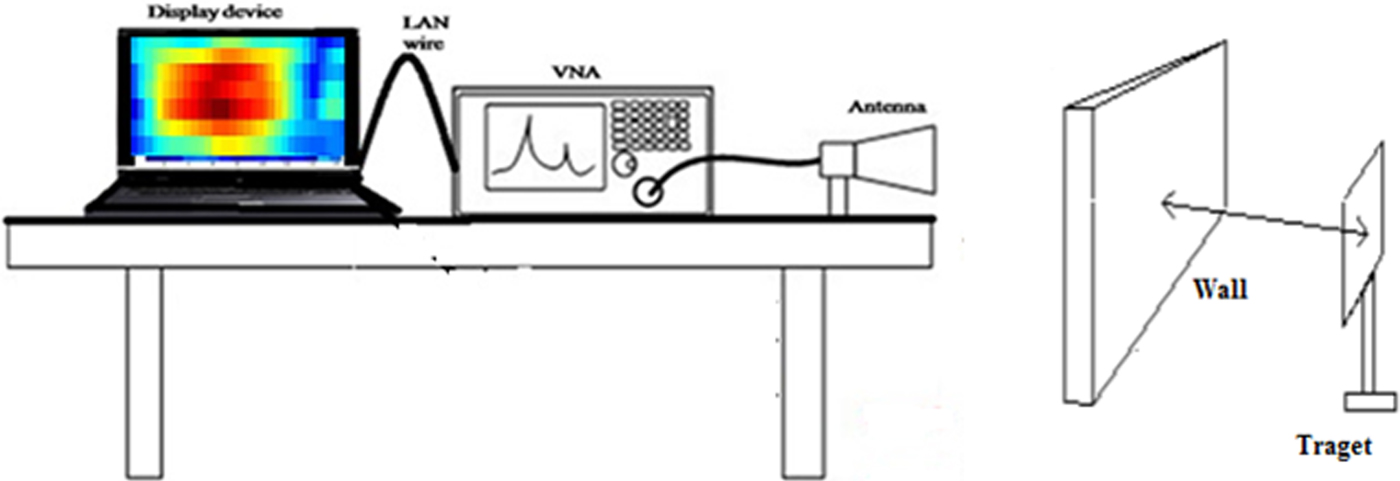
The antenna is connected to the vector network analyzer (VNA) using a coaxial cable and the antenna is positioned on a scanner for data collection. It is important to perform calibration of VNA before its operation to obtain error-free results. The calibration of VNA eliminates systematic and reproducible errors from the measurement results. Calibration plays an important role in determining the accuracy of the measurement system. A calibration kit of Anritsu model OSLN50 has been used for open, load, and short calibration of Port. After the calibration is completed we need to scan the scene. The entire arrangement is shown in Fig. 1.

Fig. 1. Experimental arrangement of the TWI system.
A metal triangular and rectangular sheet, as shown in Fig. 2, is mounted on the wooden frame and kept on the other side of the wall at the antenna aperture. The distance between the antenna and wall is kept as 60 cm and the target is kept at a distance of 90 cm from the other side of the wall. It is to be noted that the whole arrangement is made in an indoor environment and also the operating parametric conditions of the entire system used for the observations are given in Table 1.
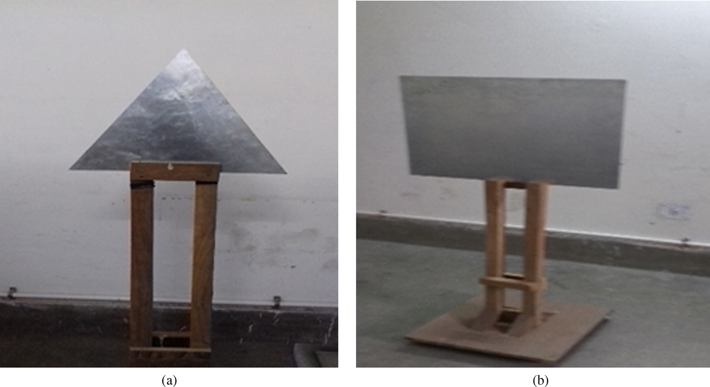
Fig. 2. (a) Triangular metal target and (b) rectangular metal target.
Table 1. System parameter values

Conventional theory and technique
The idea is to generate the high-resolution image of the metal object kept behind the wall using a stepped frequency continuous wave (SFCW) radar and it is important to understand that the image quality depends upon the correct estimation of unknown wall thickness and its dielectric constant [Reference Soldovieri, Prisco and Solimene1–Reference Dehmollaian and Sarabandi4]. The various scanning techniques being used are as follows:
Step 1: A-scan method
The target range is generated, and also, the wall parameters like its thickness and dielectric constant may be estimated by the A-scan method [Reference Kaushal and Singh10]. The complex radar signal in the frequency domain (1–3 GHz) is converted into the time domain by inverse fast Fourier transformation (IFFT) and then is mapped to the spatial domain. The signal returned from the target at a certain distance in the frequency domain is given by [Reference Agarwal, Bisht, Singh and Pathak11]
 $$D(\,f_n) = \displaystyle{1 \over {\tau _{max}}}\int_0^{\tau _{max}} {D(t)\exp ( - j2\pi f_nt)dt}, $$
 $$\Delta \tau = \displaystyle{1 \over {N_f\Delta f}},$$
 $$\tau _{max} = \displaystyle{{N_f - 1} \over {BW}},$$
where Δτ is the time resolution possible with the stepped frequency waveform of uniform steps of Δf, τ max is the maximum time possible, and BW is the bandwidth of the system. In the present case, N f = 201 and Δf = 10 MHz.
Step 2: Applying IFFT
The signal obtained in the frequency domain is converted into time domain by performing IFFT. The obtained time domain signal may be represented by
 $$s(t) = \sum\limits_{n = 0}^{N_f - 1} {S(\,f_n)\exp (\,j2\pi f_nt)}. $$
Step 3: Mapping to spatial domain
Mapping from the time domain to the spatial domain is performed according to the following equation:
 $$z = \displaystyle{{ct} \over 2}.$$
The mapped spatial domain signal is represented as:
 $$s(z) = \sum\limits_{n = 0}^{N_f - 1} {S(\,f_n)} \exp \left( {\,j2\pi f_n\left( {\displaystyle{{2z} \over c}} \right)} \right).$$
Therefore, from equation (6), the target range may be estimated, which provides approximate wall thickness. The analysis initiates with the A-scan method which provides the target location in downrange in meters as shown in Fig. 3, the peaks show the reflection from various interferences, in terms of intensity. The first peak shows the air-antenna interference, second and third peaks show the front wall and back wall reflections, respectively, from where the approximate wall thickness may be calculated, whereas, the next peak shows the target location.
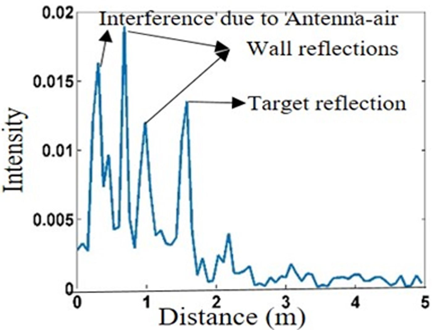
Fig. 3. A-scan image of the target behind the wall.
From Fig. 3, it is observed that the second and third reflections, which correspond to front and back walls respectively, are obtained as 0.825 and 1.05 m, therefore, the wall thickness can be estimated as 1.05 − 0.825 = 0.225 m, but the range resolution of the system is ΔR = C/2BW = 7.5 cm, where C is the velocity of the electromagnetic wave in free space and BW is the bandwidth, so that reflection is obtained as the multiple of 7.5 cm. Now, the wall thickness can be assumed anywhere between >15 cm and <22.5 cm. It is assumed to be 18 cm and the dielectric constant of the brick wall is 4 for our consideration of analysis.
Image formation using the delay–sum algorithm
There are lots of imaging techniques are available in the literature: microwave imaging techniques likes ω–k [Reference Qiu, Hu and Ding12], back projection, sum–delay beamforming [Reference Rau and McClellan13–Reference Debes, Hahn, Zoubir and Amin15], etc. However, the implementation of these techniques is applicable upon the user's requirement and parameters. In the current work, we have applied the delay and sum beam forming algorithm for the generation of high-resolution image of an object behind the wall. The delay and sum algorithm has been derived from the beamforming algorithm which has been applied to TWI systems [Reference Debes, Hahn, Zoubir and Amin15, Reference Ahmad, Amin and Kassam16]. The basic idea is to use synthetic aperture radar (SAR) for simulating a large directional antenna. This algorithm works in the frequency domain as opposed to back projection which works in the time domain. The region to be imaged behind the wall is divided into voxels and a 2D horizontal or vertical grid is formed as shown in Fig. 4, where, y a is the antenna location, (x t, y t) is the target pixel position, and R_w is the center of the antenna scanning position to the center of the voxel grid. The pixel size of the voxel grid is 59 × 15.

Fig. 4. Real-time imaging geometry for the delay–sum algorithm.
For each voxel, the distance and the corresponding delay is calculated from each radar location according to below equation:
 $$\tau _q = \displaystyle{{2R_n} \over C},$$
where C is the velocity of the electromagnetic wave and R n has been calculated as shown in Fig. 4.
The delay calculated using equation (7) is then applied to the signal received at each radar location. Coherent summation is carried out for the calculation of the intensity value of that voxel using the calculated delay. Here, the effect of the wall has been ignored. If the wall effect is considered, then the focusing delay depends upon the dielectric constant and the thickness of the wall [Reference Ahmad, Amin and Kassam16]. Therefore, the wall parameters play the crucial role to generate the focused image behind the wall.
For the SFCW system, the expression for the intensity value of the voxel at (x t, y t) is given as:
 $$S(x,\,y) = \sum\limits_{n = 1}^N {\sum\limits_{k = 1}^K {S_n}} \exp ( - 2j\omega _k\tau _q),$$
where S n is the signal received when the radar is at nth location and τ q is the focusing delay calculated for the voxel located at (x t, y t).
N is the number of positions on the scanner at which the radar is kept in monostatic mode.
K is the number of frequency points of the SFCW signal. The delay–sum algorithm can be implemented as follows:
• Calculate the distance of each voxel from all the antenna locations by considering the effect of the wall.
• For data collected at each antenna location at all SFCW frequency points, apply the delay according to the distance calculated in the above step.
• Sum the received data for all the frequency points.
• Repeat above steps for all the antenna locations.
• Sum the results obtained for all antenna locations to form the final image.
Proposed technique
The method and proposed technique is composed of different steps, as, it starts from detecting the target location, estimating the wall parameters like its thickness and dielectric constant. Later, the image of the target is generated by applying the delay–sum beamforming algorithm for the estimated wall parameters, and also, the image generated is compared with the images formed for the different values of wall parameters on the basis of the peak signal to noise ratio (PSNR). The autofocusing approach is achieved by applying the optimization technique like curve fitting and the GA.
PSNR calculation
Now, the wall thickness is varied from 15 to 23 cm and the dielectric constant is varied from 3 to 7 and C-scan images of the same target are generated accordingly. The PSNR has been considered as a comparative parameter of the different C-scan images. Initially, wall thickness of 18 cm and dielectric constant of 4, have been considered as a reference image for the PSNR calculation. Accordingly, the mean square error (MSE) and hence PSNR is calculated using the following equations [Reference Smith Steven17]:
 $$MSE = \displaystyle{1 \over {M \times N}}(\sigma _r - \sigma _n)^2,$$
 $$PSNR(\hbox{dB}) = 10\log \left( {\displaystyle{1 \over {MSE}}} \right),$$
where σ r and σ n are the standard deviation of the reference image and image with different wall parameters, respectively. M and N are the dimensions of the image. The normalized plot of the PSNR with different values of wall parameters is shown in Fig. 5. Several readings have been taken for triangular metal target and the same value of the PSNR has been obtained, as shown in Fig. 5.
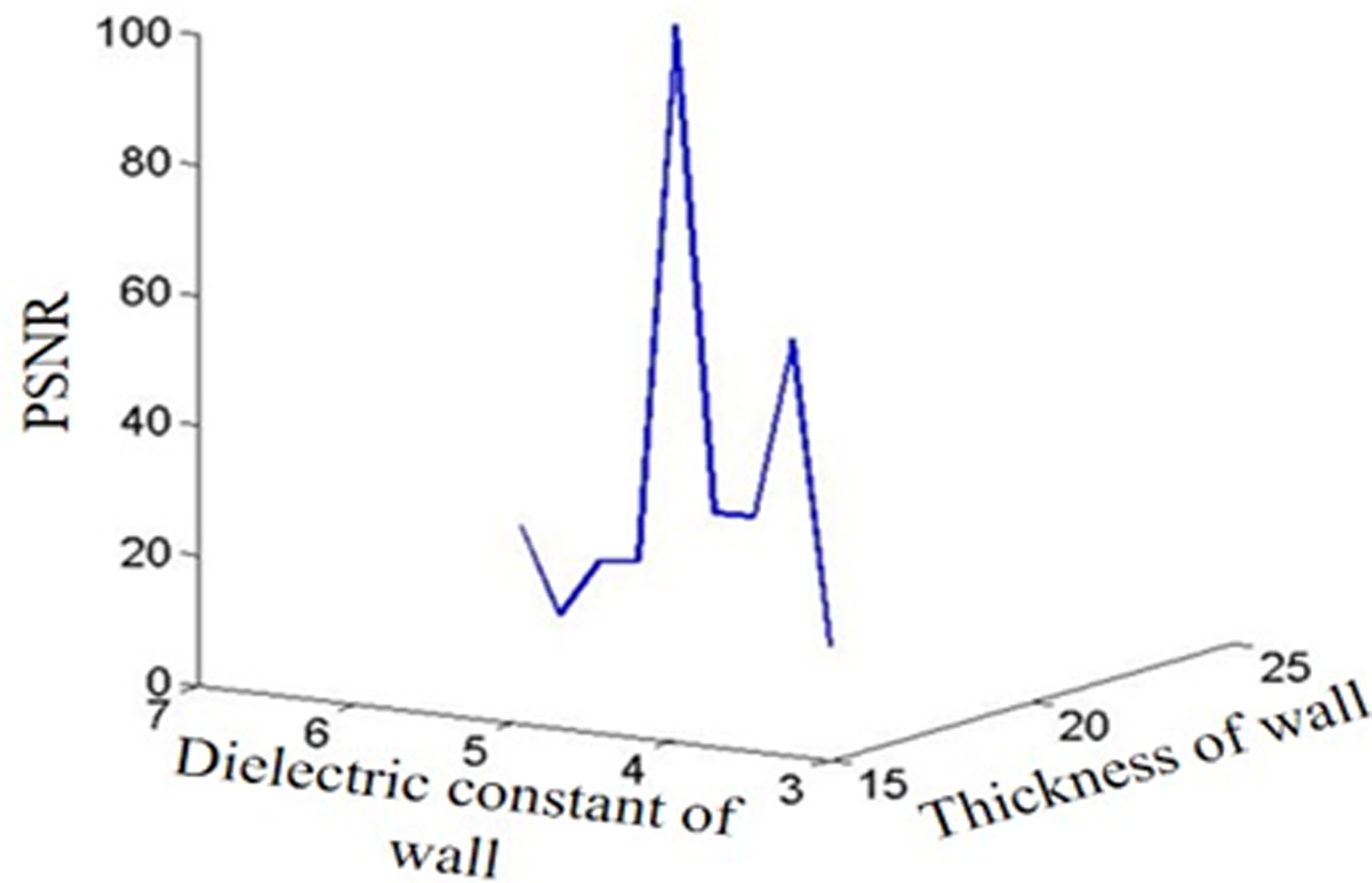
Fig. 5. PSNR values at different thickness and dielectric values.
Wall parameter adjustment using the GA
It is essential to optimize the PSNR for unknown wall thickness and dielectric constant. Let us now, consider the wall ambiguities so that wall thickness and dielectric constant due to ambiguities be t′ = t ± Δt and d′ = d ± Δd, respectively. The variation of wall thickness is Δt and that of dielectric constant is Δd. It is to be noted that any variation of wall parameters affects the image resolution and hence the PSNR.
Practically, in real life the wall thickness and dielectric constant are unknown, therefore, it is essential to optimize the PSNR for unknown wall parameters. The curve fitting optimization tool has been used for this, where, PSNR is a function of wall thickness “t” and dielectric constant “d” for developing the empirical relation with coefficient of determination (R 2) value close to 0.9 for the PSNR and wall parameters are as follows [Reference Kumar, Upadhyay and Singh18]:
 $$PSNR = a1\,\hbox{exp} - \left( {\displaystyle{{t - b1} \over {c1}}} \right)^2 \,+ \,a2\,\hbox{exp} - \left( {\displaystyle{{d - b2} \over {c2}}} \right)^2,$$
where a1, a2, b1, b2, c1, and c2 are constants, which are calculated using the curve fitting approach for R 2 values near to 0.9. Four different types of targets like rectangular, circular, triangular, and square have been considered. In total, 20 readings have been taken, five for each target. PSNR values have been obtained for each dataset according to equations (9) and (10). These PSNR values have been applied in equation (11) for calculating the constant value using the curve fitting approach. Now, the values of a1, b1, c1, a2, b2, and c2 of equation (11) have been replaced by average value of these obtained constants. The average value of the constants a1, b1, c1, a2, b2, and c2 are −0.05592, 0.175, 0.4789, 0.7411, 204.8, and −0.0868, respectively. After deriving the mathematical relation of PSNR using the curve fitting approach, next step is to find the best value of PSNR such that it should be maximized. For this purpose, GA [Reference Capelli, Riba, Rupérez and Sanllehí19, Reference Mahlab, Shamir and Caulfield20] has been applied. GA is an optimization technique that is used for large-scale optimization problems and the principles are applied to provide the best solution that motivated researchers to explore GA in imaging and pattern recognition [Reference Mahlab, Shamir and Caulfield20]. Now, taking the wall ambiguities in consideration, so that wall thickness and dielectric constant due to ambiguities be t′ = 18 ± Δt and d′ = 4 ± Δd, respectively. The variation of wall thickness is Δt and that of dielectric constant is Δd. It is to be noted that any variation of wall parameters affects the image resolution and hence PSNR. Further, the globally iterative numerical optimization method has been used for the optimization of PSNR function. The main significant feature of the GA is that it has arbitrary constituents that test for solutions outside the current minimum while the algorithm converges. In this problem, the lower and upper bounds for all the constraints of PSNR are taken as 10 and 100%, respectively. Now, the PSNR equation is given below after putting new wall parameters as equation (12):
 $$Y\lpar {{\rm \Delta} t,\,{\rm \Delta} d} \rpar = a1\,\hbox{exp} - \left( {\displaystyle{{{t}^{\prime} - b1} \over {c1}}} \right)^2 + \,a2\,\hbox{exp} - \left( {\displaystyle{{{d}^{\prime} - b2} \over {c2}}} \right)^2.$$
In genetic optimization algorithm problem, function Y(Δt, Δd) has been used, where Y(Δt, Δd) is the PSNR value. Our main aim is to maximize Y(Δt, Δd) for the optimum value of (Δt, Δd). For this, the goal has been set such that Y(Δt, Δd) should be lower than the upper boundary (UB = 100%) and greater than the lower boundary (LB = 10%). The goal vector can be defined as goal = [UB, LB] for fitness function Y(Δt, Δd). This gives the critical value of (Δt, Δd) such that Y(Δt, Δd) > LB and Y(Δt, Δd) < UB. Finding unknown variables (Δt, Δd) that optimize the objective function Y(Δt, Δd) such that Y(Δt, Δd) is maximized. After optimization, the obtained values of Δt and Δd are 1 and 1.5, respectively. Now, the corrections of wall parameters have been done; correction of the wall parameters results in new value with new thickness, which is 19 cm and the dielectric constant is 5.5. The complete flow chart of the algorithm is shown in Fig. 6.

Fig. 6. Flowchart of the proposed method.
Results and discussion
The raw data have been generated to scan the target behind the wall at 30 horizontal positions and 15 vertical positions at every 5 cm of scanning steps. The next step is to generate the high-resolution image of the triangular and rectangular metal using the delay–sum algorithm. Figure 7 shows the image of metallic triangular target behind the wall, obtained using the delay–sum algorithm without considering the wall effect. From Fig. 3, the approximate wall thickness has been assumed, i.e. 18 cm, and, also the dielectric constant is assumed to be 4. Now, the delay–sum algorithm has been applied to generate an image as shown in Fig. 8, which seems a defocused image. For obtaining a focused image, the method followed is that, the dielectric constant and the wall thickness are varied from 3 to 7 and 15 to 23 cm, respectively. For each new value of the wall parameter, the target image is generated and further compared with Fig. 8, which has been considered as the reference image. It is to be noted that the comparison is based on the image quality, as, PSNR being the measuring parameter. Later, the curve fitting approach and GA have been applied to maximize the PSNR value for different wall thickness and dielectric constant values, using equation (12). It is observed that, the maximum PSNR value has been obtained for the wall thickness of 19 cm and dielectric value of 5.5. These parameters are considered for the delay–sum algorithm, and, hence the image shown in Fig. 9 is obtained, which is a more focused image in comparison with the previous image. A better focused image of the new target, i.e. rectangular metal sheet has been generated, as shown in Fig. 10.
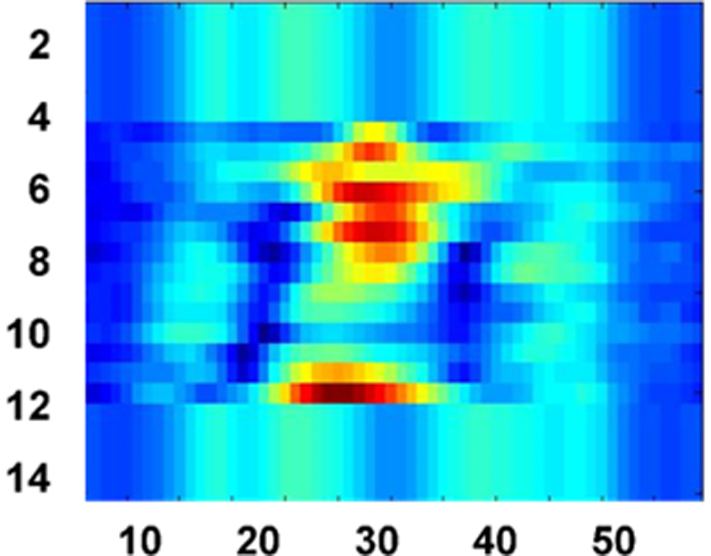
Fig. 7. C-scan image of the triangular target without the considering wall effect.
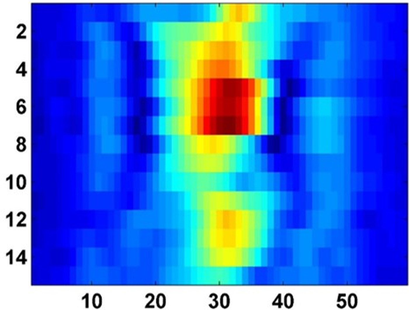
Fig. 8. C-scan image of the triangular target behind the wall at thickness t = 18 cm and dielectric value d = 4.
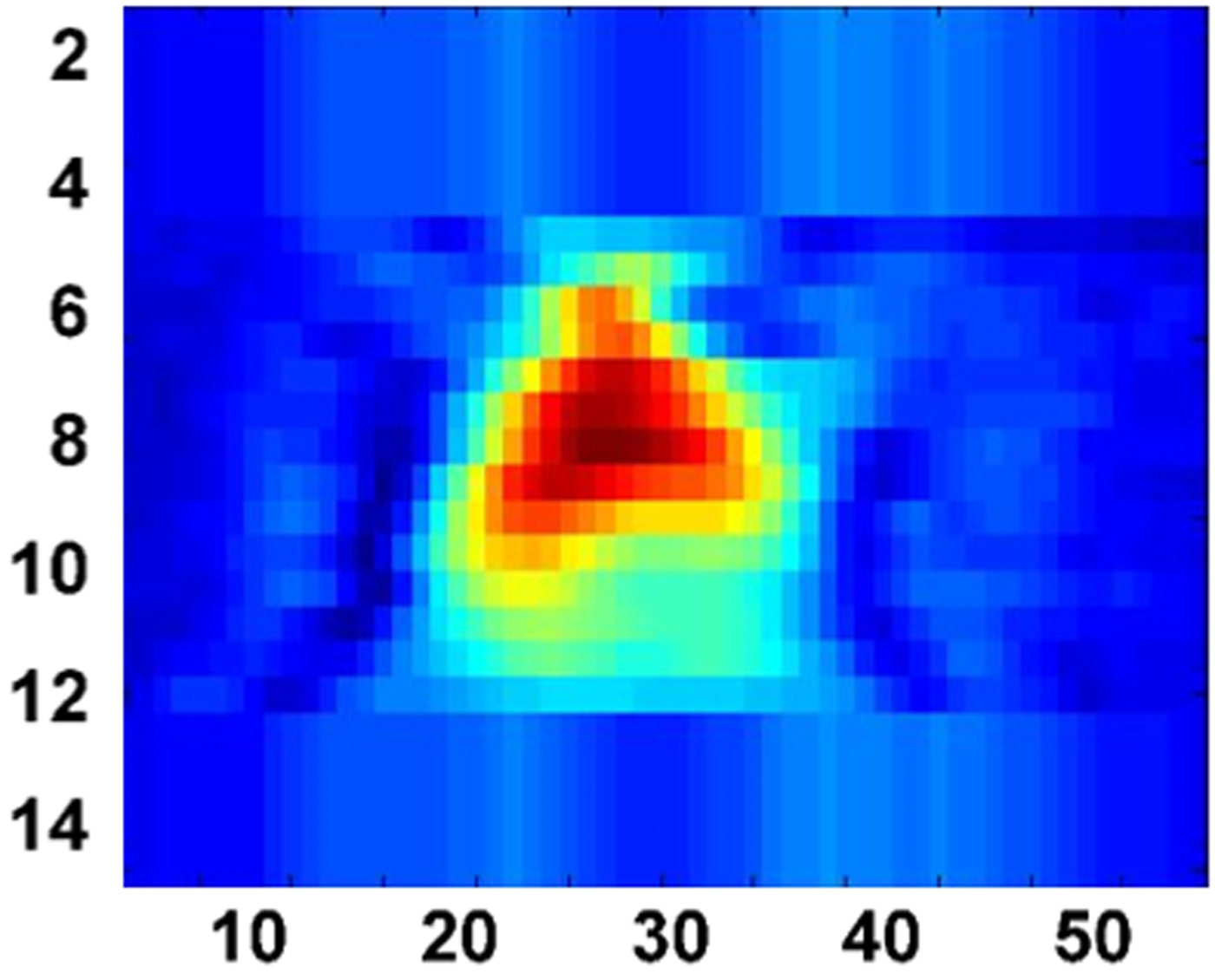
Fig. 9. C-scan image of the triangular target behind the wall at thickness t = 19 cm and dielectric d = 5.5.
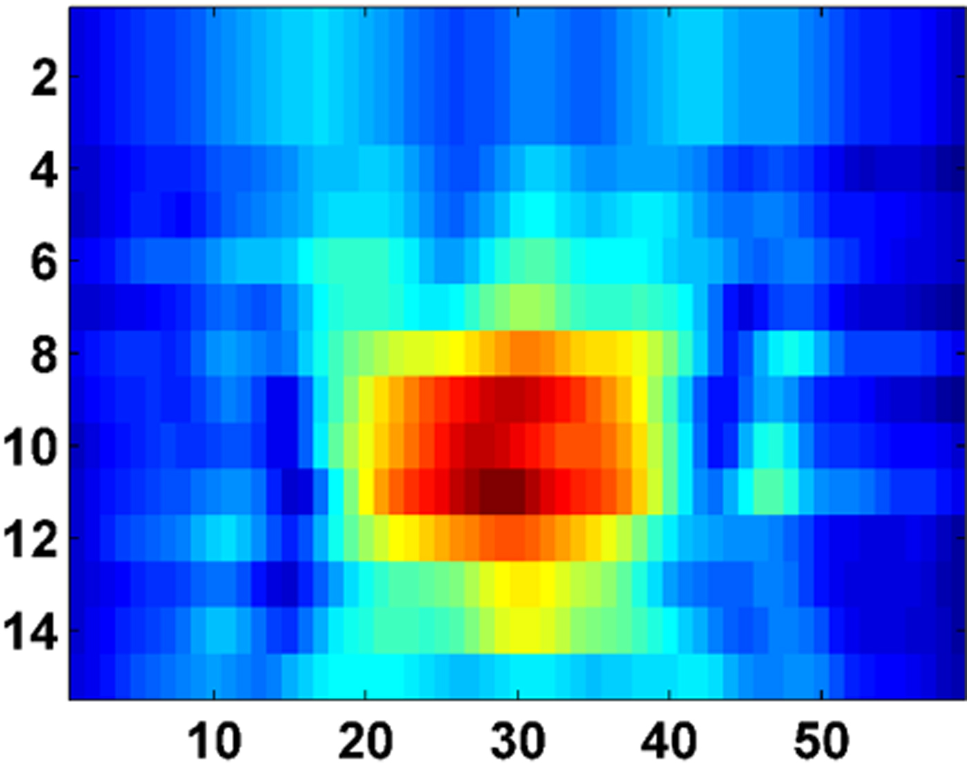
Fig. 10. C-scan image of the rectangular target behind the wall at thickness t = 19 cm and dielectric d = 5.5.
Conclusion
The method and approach followed is the combination of real-time experimental work being carried out along with the deep critical analysis of the observations and results. The articulate work concludes that the wall ambiguities affect the image quality, as, incorrect estimation of the wall thickness and dielectric constant leads to the blurriness of the image. Curve fitting and GA have been used to maximize the PSNR of images, which is the figure of merit to obtain a better quality image. The new autofocusing approach presented here is less complex and takes few minutes for simulation. Though, enough work has been done previously, but, it has been observed that B-scan images were taken previously into the consideration for analysis, whereas, the current work has been carried out by C-scan, which has put a new benchmark in the field of TWI. Finally, an autofocusing imaging system with appropriate delay–sum algorithms has been developed for through-wall imaging. It is concluded that the algorithm and the method followed in the current work for autofocusing correct the wall parameter ambiguities to generate the correct and actual image of the target.
 Sandeep Kaushal hails from a small town in Punjab (India). He completed his B.E. (Electronics) from North Maharashtra University, Maharashtra. Then, he worked for 2 years and joined the teaching profession in 2003 and later earned an M.Tech. (ECE) and an MBA (HRM). He also earned a Ph.D. in Uttarakhand Technical University, Dehradun in 2010. He has expertise in the field of optical fibers communication, biomedical image processing, wireless technologies and microwave radar technology & applications. He has published more than 40 research articles in various conferences and journals. Currently, he is working as an Associate Professor in the Department of ECE at ACET, Amritsar (Punjab), India.
 Bambam Kumar hails from Bihar, India. He received his Ph.D. degree in hidden object detection through microwave and MMW imaging from the Indian Institute of Technology Roorkee (IIT Roorkee), Roorkee, India. He has more than 7 years of experience in teaching. Presently, he is an Assistant Professor in the Department of Electronics and Communication Engineering, Bhagalpur College of Engineering, Bhagalpur. He received a young scientist award in 2016 organized by UCOST, Uttarakhand. His research interests include RF and microwave engineering, microwave and MMW imaging and electromagnetism. All experimental studies were carried out on through the wall imaging radar system by him.
 Dharmendra Singh received his Ph.D. degree in electronics engineering from Banaras Hindu University, Varanasi, India. He has more than 20 years of experience in teaching and research. He was a Visiting Scientist/Postdoctoral Fellow with the Information Engineering Department, Niigata University, Niigata, Japan; the German Aerospace Center, Wessling, Germany; the Institute for National Research in Informatics and Automatique, France; the Institute of Remote Sensing Applications, Beijing, China; Karlsruhe University, Karlsruhe, Germany; and UPC, Barcelona, Spain. He is currently a Professor with the Department of Electronics and Communication Engineering, Indian Institute of Technology Roorkee, Roorkee, India. He has published more than 190 papers in various national/international journals and conferences. His main research interests include microwave remote sensing, electromagnetic wave interaction with various media, polarimetric and interferometric applications of microwave data, numerical modeling, ground penetrating radar, and through-wall imaging. Through the wall imaging radar system activity was spear headed by him.