Introduction
The ecological imbalance created by ever-increasing anthropogenic pressure on the environment with respect to the slow regeneration of its resources has always been a burning issue for land use planners and environmentalists. This human-induced resource extraction is best manifested by the spatial and temporal variation of land use classes (Palchoudhuri et al. Reference Palchoudhuri, Roy and Srivastava2015). Potential land use assessment is thereby the fundamental step for sustainable land resource management (Dengiz & Sağlam Reference Dengiz and Sağlam2012). Being the primary land use, evaluating and monitoring spatio-temporal dynamics of agriculture is thereby the major concern for most land use planners and environmentalists. Therefore, knowledge of spatial location and distribution of crops at global, national and regional scale is a pre-requisite for any agricultural assessment application. Records of crop types, usually reflected as crop maps, are an invaluable source for any national or regional agricultural boards and insurance agencies. This inventory serves the purpose of yield estimation (Becker-Reshef et al. Reference Becker-Reshef, Vermote, Lindeman and Justice2010; Kogan et al. Reference Kogan, Kussul, Adamenko, Skakun, Kravchenko, Krivobok, Shelestov, Kolotii, Kussul and Lavrenyuk2013), assembling crop phenology statistics (Gallego et al. Reference Gallego, Kravchenko, Kussul, Skakun, Shelestov and Grypych2012, Reference Gallego, Kussul, Skakun, Kravchenko, Shelestov and Kussul2014), crop rotation records, assessing soil fertility (Löw et al. Reference Löw, Michel, Dech and Conrad2013; Ustuner et al. Reference Ustuner, Sanli, Abdikan, Esetlili and Kurucu2014), identifying factors of crop damage or stress due to disease, mineral deficiency, drought or bad weather (Kussul et al. Reference Kussul, Skakun, Shelestov, Lavreniuk, Yailymov and Kussul2015).
Remote sensing (RS) images, particularly from space-borne satellites, have always been a promising source of knowledge for analysing spatio-temporal variability of any biophysical parameter (Dhumal et al. Reference Dhumal, Rajendra, Kale and Mehrotra2013). Along with a synoptic view, RS can provide evidence on the health of vegetation and identify changes in phenology between fields as well as between different crop types. Thus, due to its capacity to acquire timely images, providing repeated measurements of crop phenology, it plays a significant role in assessing crop health, providing crop classification or potential yield estimation.
The traditional approach to crop classification with RS data has been primarily based on supervised and unsupervised classification techniques to map geographic distribution of crops. Remote sensing images represent the features on Earth with respect to their corresponding spectral reflectance, known as a spectral signature (Al-doski et al. Reference Al-doski, Mansor and Shafri2013). Based on the same concept, any two different crop types would also exhibit differing spectral signatures, which can be used to distinguish them in RS classification. In plant species, this difference in signature is due to their phenology (accumulation of biomass), leaf orientation and canopy structure. In RS, multi-temporal spectral information from red and infrared and their ratio indices (vegetation indices (VIs)) has been used successfully to assess plant phenology (Jackson & Huete Reference Jackson and Huete1991). Meneses-Tovar (Reference Meneses-Tovar2011) and Palchowdhuri et al. (Reference Palchowdhuri, Vyas, Kushwaha, Roy and Roy2016) identified significant relationships between plant biomass growth and normalized difference vegetation index (NDVI), derived from satellite images to assess the health of vegetation. Since the launch of Landsat-1 in 1972, multi-sensor and multi-resolution remote sensed images have provided crop type information (Bauer & Cipra Reference Bauer and Cipra1973; Jewell Reference Jewell1989). With the promotion of higher resolution sensors with time such as RapidEye (2008), GeoEye-1 (2008), WorldView-2 (2009), Landsat-8 (2013), SPOT-7 (2014) and Sentinel-2 (2015), data acquisition has become faster, more up-to-date and more cost-effective. Itzerott & Kaden (Reference Itzerott, Kaden and Braun2006) considered assessing spectral curves to distinguish 12 crop types from a time-series of 35 Landsat-TM scenes for 1987 to 2002. Odenweller & Johnson (Reference Odenweller and Johnson1984) assessed multi-temporal Landsat images in the US Corn Belt and analysed the spectral profile of a green vegetation indicator of specific annual crops, such as winter cereal and sunflowers. Serra & Pons (Reference Serra and Pons2008) supported the use of a multi-temporal approach as well as phenology data in any crop classification methodology. The method used by Zhong et al. (Reference Zhong, Gong and Biging2014) was based on spectral and phenological metric indices representing multi-temporal information with only a single year training set. According to Knight et al. (Reference Knight, Lunetta, Ediriwickrema and Khorram2006), phenology plays a critical role in classifying and generating accurate crop maps. Li et al. (Reference Li, Wang, Zhang and Lu2015b ) also endorsed an enhanced time series of NDVI to be analysed in a decision tree (DT) environment to obtain a classification accuracy >90%.
A multi-temporal series data for tracking plant phenology during the cropping window as well as high spatial and spectral resolution is, therefore, a prerequisite to any crop classification effort. Time-series data of the study site incorporates the growth stage of the phenology cycle, whereas the spectral and spatial information is useful for accurate identification of crop types (differentiating from one another spectrally and spatially). Vinciková et al. (Reference Vinciková, Hais, Brom, Procházka and Pecharová2010) and Singha et al. (Reference Singha, Wu and Zhang2016) investigated the effect of phenology combined with high-resolution multi-spectral (MS) data to accurately classify crops. Time-series MS data from MODIS & NOAA-AVHRR (coarse spatial resolution), Landsat (medium spatial resolution), IRS & SPOT (high spatial resolution) and WorldView-2 (very high spatial resolution) have been used in many studies at the national and sub-national level for precision agriculture mapping (Upadhyay et al. Reference Upadhyay, Ghosh, Kumar, Roy and Gilbert2012; Son et al. Reference Son, Chen, Chen, Duc and Chang2014; Wang et al. Reference Wang, Xiao, Qin, Dong, Zhang, Kou, Jin, Zhou and Zhang2015). A recent addition to the medium to high spatial resolution sensors is the ESA's (European Space Agency) Sentinel-2 images. Due to their high spectral (13 bands-visible, near infrared (NIR) and short wave Infra-red spectrum) and temporal resolution (5-day revisit), these data have immense potential for temporal evolution of the two most prime bio-physical parameters that define a particular crop type; chlorophyll content and leaf area index (LAI) (Frampton et al. Reference Frampton, Dash, Watmough and Milton2013; Majasalmi & Rautiainen Reference Majasalmi and Rautiainen2016). Immitzer et al. (Reference Immitzer, Vuolo and Atzberger2016) ascertained the potential of Sentinel-2 in extracting the crop type information, useful for parameterizing crop growth models for yield estimation and agricultural statistics.
These special traits (image resolution, repeat cycle, etc.) of very high resolution (VHR) sensors (WorldView, GeoEye) have always proved to have potential for the Control with RS (CwRS) programme, a significant component for verifying of European Union's Common Agricultural Policy (CAP) applications by farmers in Europe (Chmiel et al. Reference Chmiel, Kay, Spruyt and Altan2004). The CAP supported by EU provides a range of Price guarantees and Direct Payments to farmers, representing >0·40 of the EU budget. Each Member State of the EU is responsible for subsidy administration and control; CwRS, being one of the accepted control programmes for administering CAP subsidies, uses the remote-sensing high-resolution data to extract farm information digitally. Under this CwRS campaign, an attempt has been made to develop a methodology for a high-resolution sub-parcel crop diversification in the UK at a regional scale of 1 : 10 000. The current study adopts a semi-automatic integrated spectral statistical model in order to validate the crop types using their spectral signatures.
Conventional classification mainly includes the supervised classifiers that use the maximum-likelihood (ML) algorithm. However, because of the recent accessibility of fine resolution data, these conventional classifiers could no longer decipher the complexity of such informative data (Lloyd et al. Reference Lloyd, Berberoglu, Curran and Atkinson2004). To resolve such issues, studies nowadays use object-based or machine learning algorithms to identify features from RS (Li et al. Reference Li, Ke, Gong and Li2015a ). Therefore, in the current approach, Decision Tree (DT) learning and the Random forest (RF) algorithm, being the most representative machine-learning procedure that is noise-free and subject to minimum overfitting (Arminger et al. Reference Arminger, Enache and Bonne1997; Watts & Lawrence Reference Watts and Lawrence2008), has been integrated for the first time into a statistical framework to assess various spectral VIs as a signature to identify each crop type. The current research paper illustrates a case-study for the above-mentioned hybrid modelling approach of a sub-parcel crop classification in the Coalville region of England (UK). As a part of the 2016 CwRS programme, Coalville was among 15 zones considered for crop diversification using Earth Observation. It was chosen as the study area because of its central location in England and predominantly agrarian land use, to showcase the influence of high-resolution satellite information and machine learning technology on deciphering the major crop types and their distribution. The output crop map would hold a significant influence on any agricultural assessment application including crop stress management, field potential, or yield estimation.
Materials and methods
Study area
The current study was carried out in Coalville, in northwest Leicestershire, in central England (Upper Left: 52° 46′ N; −1° 33′ W; Lower Right: 52° 35′ N; −1° 15′ W) and it covers an area of 400 km2 (Fig. 1). The region is characterized by a temperate climate with an average annual temperature of 9·2 °C and 699 mm of mean annual rainfall. The landform of the area is typical of the gently rolling farmland associated with the Leicestershire countryside; local watercourses, including the River Sence and River Mease which run east to west in the south of the study area, and are interspaced by farm valleys. Bardon Hill creates a prominent landform to the east of Coalville, characterized by its evergreen forest plantation and a granite quarry. The predominant land use of the zone is grassland; the major crop types grown in the zone are barley, wheat, oat, oilseed, maize, peas and field beans.

Fig. 1. Study area, Coalville, UK.
Dataset
Ground truth
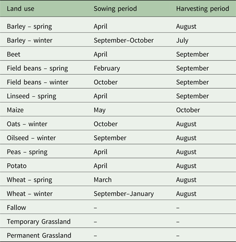
A polygon vector dataset of the rural land register (RLR), consisting of agricultural parcels (plots) with attributes of growing crop types and its area updated by regional farmers for claiming the Single Payment Scheme as an integral part of the Common Agricultural Policy (CAP) of EU, was provided by the Rural Payments Agency (RPA) for the study area, and used as ancillary data to support the ground truth. The RPA also provided a parcel boundary layer (PBL) as a vector dataset throughout the zone to represent the agricultural parcels. Multi-crop parcels from both RLR and PBL datasets were split with respect to each crop type boundary under the same parcel IDs, representing each crop type as a separate polygon entity. Assessment of the farmers’ claims revealed 27 crop types grown in the study area, of which 16 were considered for classification purposes because of their popularity within the zone (Table 1). An extensive field survey was carried out from mid-May to June 2016 over the study area. Stratification based on the most and least frequently claimed crop types and conditioned by field accessibility (proximity to road connectivity), as well as cloud-free locations on the satellite data, was implemented by applying RS and geographic information system (GIS) techniques. Altogether, 596 samples of crops were chosen throughout the area to be verified on the ground based on the above conditions. Claimed crops were verified for those selected samples in the field by surveyors and were used as valid ground truth parcels for executing and validating the classification model. Out of 596, 311 samples of crop types were used to train the classifier and the remaining 285 samples applied for classification validation (Fig. 2).

Fig. 2. Ground truth sample distribution for training and validation.
Table 1. Land use classification in Coalville, UK, 2016
Satellite data and pre-processing
Three optical satellite images, one from WorldView-3 (WV-3) and two from Sentinel-2A (S2), covering the cropping season (Table 1) were used in the current study. Data were selected based on data availability, the proportion of cloud cover (<0·05) and the vegetation phenology period for the chosen crops (Table 1) over the study area. Areas falling under cloud were also masked out of the scene due to its detrimental effect on classification. The choice of these sensors, S2 and WV-3, was also to showcase the integration of multi-sensor data and its impact on classification accuracy and to show how the finer spectral resolution of S2 can be used to refine the classification result based on broad bands of red and NIR of WV-3. The WV-3 MS image was acquired in April 2016 and S2 images were acquired in June and July 2016 over the study area. WV-3 is a commercial Earth Observation satellite developed by DigitalGlobe Inc., (Longmont, CO, USA) and launched in August 2014. It is a very high spatial resolution MS satellite sensor with eight MS bands (400–1040 nm) at 1·24 m, eight shortwave-infrared (SWIR) bands (1195–2365 nm) at 3·7 m, one panchromatic band (450–800 nm) at 0·31 m and 12 ‘Clouds, Aerosols, Vapours, Ice and Snow’ (CAVIS) bands (405–2245 nm) at 30 m. The satellite has a swath width of 13·1 km, an off-nadir angle of 20°, an average revisit time of <1 day and capturing 6 80 000 km2 of imagery per day. The chosen WV-3 was a Standard Imagery (2A) MS 4 band (Blue, Green, Red and Infrared) data from Digital Globe as provided by the Joint Research Centre covering the study area of 400 km2 by two non-overlapping tiles. After importing the tiles in *.img format and constructing a mosaic image, a seamless scene of WV3 data for the study area was generated. The orthorectification process was performed in ERDAS Imagine, version 15 using the Worldview Rational Polynomial Coefficient model (2nd order Polynomial) as well as the OS Terrain 5 m Digital Elevation Model for elevation info and collecting ground control points from the reference ordinance survey master map following a sub-pixel root mean square error accuracy.
S2 was launched in June 2015 by the European Space Agency (ESA). It is a MS and high spatial resolution satellite which is part of Copernicus, the European Commission's Earth Observation Programme (Drusch et al. Reference Drusch, Del Bello, Carlier, Colin, Fernandez, Gascon, Hoersch, Isola, Laberinti, Martimort, Meygret, Spoto, Sy, Marchese and Bargellini2012). The MS Sensor of Sentinel-2 has 13 spectral bands; four visible (VIS) and NIR bands at 10 m, six red-edge SWIR bands with spatial resolution of 20 m and three atmospheric bands with 60 m resolution (Drusch et al. Reference Drusch, Del Bello, Carlier, Colin, Fernandez, Gascon, Hoersch, Isola, Laberinti, Martimort, Meygret, Spoto, Sy, Marchese and Bargellini2012). The S2 MS images were downloaded from the ESA Sentinels Scientific Data Hub website as Level 1C top-of-atmosphere reflectance tiles, which are 100 km2 orthorectified images in UTM/WGS 84 projection (European Space Agency 2015). The current study followed the British National Grid coordinate system; therefore, the S2 data downloaded was re-projected accordingly from its UTM projection. Due to the multi-resolution of the data, both WorldView and Sentinel images were re-scaled to 2 m scale (cell size modification, values being unaffected) and were applied to evaluate the potential of visible and NIR bands in the classification process. The data pre-processing also involved masking out of non-agricultural areas including natural vegetation, waterbodies and man-made features in order to reduce the impact of mixed pixels (reflectance caused by non-agricultural areas) on crop classification accuracy.
Vegetation indices
Vegetation indices have been used widely in RS for a range of applications such as vegetation monitoring (Fensholt & Proud Reference Fensholt and Proud2012; Lu et al. Reference Lu, Kuenzer, Wang, Guo and Li2015), drought studies (Sánchez et al. Reference Sánchez, González-Zamora, Piles and Martínez-Fernández2016), or climate and hydrological modelling (Diodato & Bellocchi Reference Diodato and Bellocchi2008; Kaspersen et al. Reference Kaspersen, Fensholt and Drews2015). Spectral VIs are mathematical functions of various spectral bands, covering the visible and NIR regions of the electromagnetic spectrum. The main objective of generating the time series spectral VIs was to enhance and separate photosynthetically active vegetative responses from non-vegetative reflectance throughout the cropping season from emergence to harvesting.
In the current study, three VIs were tested: the NDVI (Rouse et al. Reference Rouse, Haas, Schell, Deering, Freden, Mercanti and Becker1973); the green normalized difference vegetation Iidex, GNDVI (Gitelson et al. Reference Gitelson, Kaufman and Merzlyak1996) and the soil adjusted vegetation index, SAVI (Huete Reference Huete1988). These VIs were selected due to their significance in measuring the vigour of green vegetation, e.g. percentage cover, LAI, biomass. The choice of indices was based on the response from different crop types in the zone. For example, because SAVI adjusts the impact of soil on reflectance, spring crops in the zone can be easily separated from winter ones. Therefore their selection was also representative of the amount of biomass accumulated with time, chlorophyll content and crop health, as well as negating the impacts of soil condition.
Being a common VI, NDVI is based on the difference between the maximum absorption and reflection in the red and NIR spectral bands to quantify the vegetation's photosynthetic response (Tucker Reference Tucker1979; Sellers Reference Sellers1985). This index is calculated by the following equation:
 $$NDVI = \displaystyle{{\rho - \alpha} \over {\rho + \alpha}} $$
where ρ and α are the reflectance in NIR and red bands, respectively.
The GNDVI is a modification of the NDVI and it measures reflectance in the green band instead of the red band. It is calculated by the following equation:
 $$GNDVI = \displaystyle{{\rho - \beta} \over {\rho + \beta}} $$
where ρ and β are the reflectance in NIR and green bands.
Soil-adjusted vegetation indices were developed to reduce the soil brightness effect from spectral VIs using red and NIR wavelengths. Huete (Reference Huete1988) considered the SAVI, which contains an adjustment factor (L) in its calculation:
 $$SAVI = \displaystyle{{\rho - \alpha} \over {\rho + \alpha - L}} \times (1 + L)$$
Huete (Reference Huete1988) suggested including the optimal adjustment factor (L = 0·5), as this value has been found effective for reducing soil noise throughout a wide range of vegetation densities. For this reason, and taking into account the current study area, L was set to 0·5 in the current study.
The NDVI, GNDVI and SAVI indices were computed for the study area based on the corresponding bands for both sensors (WV3-B2 (550 nm), B3 (660 nm) and B4 (835 nm) and S2 with B3 (560 nm), B4 (665 nm) and B8 (840 nm)). In Fig. 3, the NDVI, GNDVI and SAVI layers are represented as the RGB composite of their time series values (i.e. R = T1 NDVI, G = T2 NDVI and B = T3 NDVI).

Fig. 3. Vegetation indices of NDVI, GNDVI and SAVI for Coalville.
Classification
A RF classification algorithm (Breiman Reference Breiman2001) was applied to the study area to classify the different crop types. This is an ensemble learning technique that involves a combination of several DTs designed to separate the crop types. The concept of combining many trees is more reliable for an accurate result than the use of only one tree. This process of combination ensures tree diversity because of their training with various subsets and with different split rules at their nodes. Hence, each tree within the ensemble is defined with respect to a random subset of the original data, resampling the data in the process. After that, tree nodes are separated using the best split variable selected from random predictive variables. As a result, different classification outputs are derived from each tree, and a simple majority function is used to create the final classification result. The RF technique has been used successfully in various RS applications including land cover and crop classification studies (Gislason et al. Reference Gislason, Benediktsson and Sveinsson2006; Rodriguez-Galiano et al. Reference Rodriguez-Galiano, Chica-Olmo, Abarca-Hernandez, Atkinson and Jeganathan2012a , Reference Rodriguez-Galiano, Ghimire, Rogan, Chica-Olmo and Rigol-Sanchez b ; Tatsumi et al. Reference Tatsumi, Yamashiki, Canales Torres and Ramos Taipe2015).
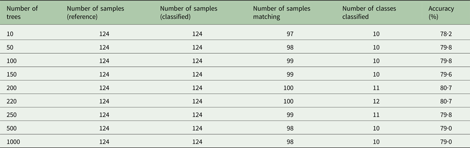
In the current study, the RF algorithm was implemented using SAGA GIS (Conrad et al. Reference Conrad, Bechtel, Bock, Dietrich, Fischer, Gerlitz, Wehberg, Wichmann and Böhner2015). Different parameters were optimized in RF; after testing its performance with various sets of trees with respect to output accuracy for a small subset of the study area (Table 2), the number of trees selected for the final classification was set to an optimum value of 220 for its highest accuracy as well as highest number of class identification. For the Coalville area, three different RF classification models were developed using the same training set but different input variables (i.e. NDVI, GNDVI and SAVI).
Table 2. Assessment of optimum number of trees for Random forest parameterization

Identification of crop types depends on temporal phenological discrimination of their spectral signatures from the representative ground samples. However, it is often found that some crop types exhibit similar responses at a particular phenological stage, even with a similar soil and moisture pattern. Also, because of the broad band-widths, MS sensors result in spectral confusion and inseparability for some crop types. Therefore in the current study, to resolve such issues, higher band ratios and spectral indices of Sentinel-2 (13 bands) were evaluated along with the above-mentioned VIs in a supervised DT modeller to improve classification accuracy. Other than Red, Green and NIR, Red Edge channels of 705, 740 and 783 nm of S2 were also used in indices to separate spectrally overlapping crops.
Hence, along with RF, the DT classifier was also tested separately to distinguish spectrally overlapping crop types in the study area. Only the misclassified crop types that resulted from the RF classifier were chosen and filtered in the DT modeller. This DT technique also uses RS data to classify Land Cover/Land Use or crop type maps (Otukei & Blaschke Reference Otukei and Blaschke2010; Punia et al. Reference Punia, Joshi and Porwal2011; Li et al. Reference Li, Wang, Zhang and Lu2015b ) following a non-parametric learning method based on a supervised concept, i.e. its basic requirements include a training dataset linking the response variable to its explanatory drivers. In RS classification, the land use area, in this case, the area under each crop type, constitutes the response variable and the spectral information identifying this represents the explanatory variables (Fig. 4).

Fig. 4. Decision tree modeller.
Both RF and the DT were executed separately in the study area to spectrally distinguish crop types in various iterations. At the end, the filtered output of the spectrally overlapping classes from the DT modeller was integrated into the RF output at parcel level in the final classified result. Four iterations were conducted altogether, and each iteration was followed by a confusion matrix that assessed the quality of the results and set a goal for the next iteration. Thus, each iteration and its results are an update of the previous one.
To evaluate the crop classification result from both methods (RF and DT), standard accuracy assessment metrics derived from a confusion matrix (between classified and ground reference data) were calculated, i.e. overall accuracy (OA), κ coefficient, producer's accuracy (PA) and user's accuracy (UA). This error matrix was standardized and recommended by Foody (Reference Foody2002), and is used commonly in the literature. Producer's accuracy relates to the probability that a reference class is correctly classified. On the other hand, the UA estimates the probability of a predicted class on a map, which matches the corresponding class on the reference data. The OA of a classification is found by relating the diagonal cells of the confusion matrix to the total number of validation samples. The κ coefficient (Tatsumi et al. Reference Tatsumi, Yamashiki, Canales Torres and Ramos Taipe2015) is calculated as follows:
 $$\kappa = \displaystyle{{P(\alpha ) - P(e)} \over {1 - P(e)}}$$
where P(α) is the proportion of cases in agreement and P(e) is the proportion of cases that are expected by chance. Therefore, κ = 1 shows that the classes are in complete agreement, however, κ = 0 indicates no agreement among classes.
Results
Random forest classifier
Normalized difference vegetation index, green normalized difference vegetation index and soil adjusted vegetation index assessment
The NDVI stack image of three time periods (April, June and July) for the study zone was used in the RF classifier as the raster input and the ground truth as the training set input in the model run with an optimum number (220) of trees. The output classified layer (Fig. 5) was a thematic raster.

Fig. 5. Crop type Classification output using NDVI, GNDVI and SAVI for Coalville.
For the study area, NDVI was found to have reduced classification accuracy for linseed-spring, maize, wheat-winter and temporary grassland crop types (Table 3). Therefore, RF was also implemented using the GNDVI index as the raster input with respect to the same training sets vector to aim for an improvement in these classes. When GNDVI was integrated with NDVI, the accuracy of all the classes mentioned, as calculated from the output, has improved (Table 3).
Table 3. Accuracy assessment (%) of the classified crop map under the study area
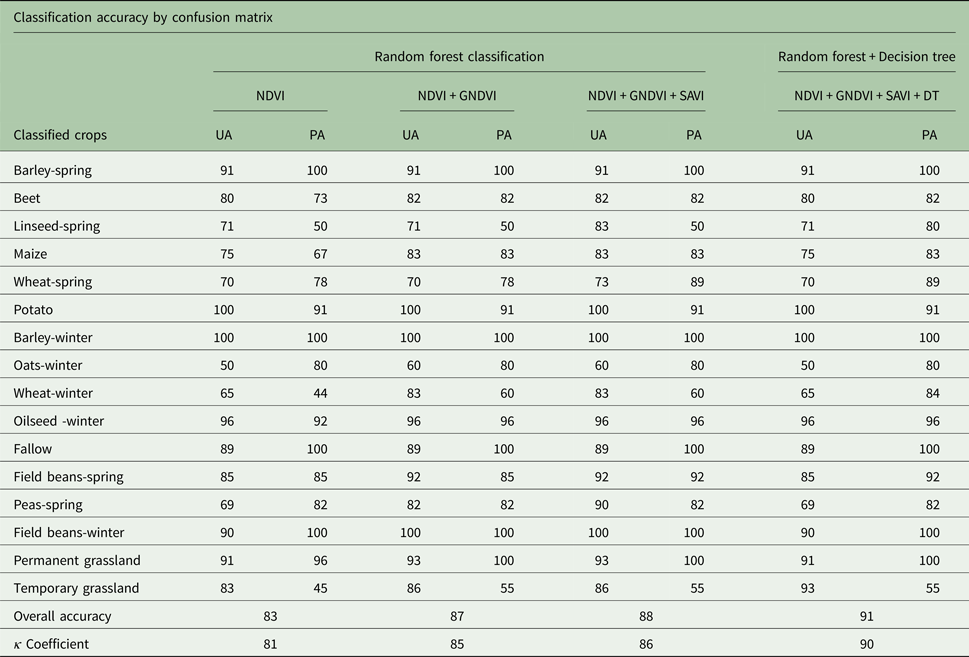
Finally, RF was also tested using the SAVI index as the raster input with respect to the same training sets vector data. Other than improving wheat-spring and field beans-spring, SAVI did not make much difference to the classification accuracy (Table 3).
Decision tree classifier
A DT algorithm was also utilized in the study area to improve those crop types that were misclassified due to similar spectral response in visible and NIR bands by the RF classifier. Combining various spectral ratios from Sentinel-2 (Band 6 to 8 with Band 3 to 5 Infrared and red narrow bandwidths) with NDVI in the DT modeller (Fig. 6), classes such as linseed-spring and wheat-winter could be spectrally filtered out from overlapping classes such as wheat-spring and oat-winter, thereby considerably increasing their producer's accuracy in the final classified layer. Finally, the output was based on the conditions set for each crop type depending on their priority within the zone.

Fig. 6. Use of Sentinel-2 for spectral filtering of wheat-winter and oats-winter in decision tree model. (a) Sentinel-2 image. (b) VHR image.
Zonal attributes
Zonal attribution was implemented using GIS to extract crop type information from the derived classified output rasters (RF and DT) with respect to each agricultural parcel boundary of the zone. The PBL representing each agricultural parcel, as a polygon with a unique ID, was used to mask out crop type information from the classified output layers. This PBL vector layer was attributed to their respective crop type and its area using a majority function on the classified raster. The output tables were considered for classification accuracy assessment with respect to the collected ground truth validation samples. Finally, the classified layer for Coalville was created as the classified land use vector layer, containing the attributes of crop name and parcel area, as extracted from the classified raster output from RF and DT (Figs 7 and 8).

Fig. 7. Classified crop map for Coalville, UK.

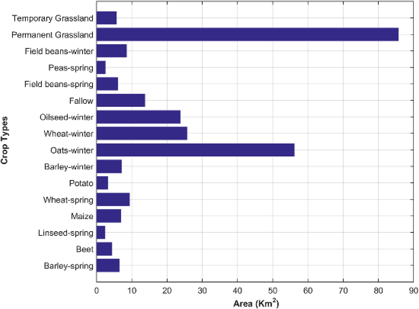
Fig. 8. Area of coverage for each classified crop.
Accuracy assessment
The confusion matrix was evaluated with each iteration (four for the study zone) in order to increase crop identification accuracy.
The first column (Table 3) is the result following classification with NDVI. With this index, crop type (linseed-spring, maize, wheat-winter and temporary grassland) were of low accuracy, with the majority of crops well represented, presenting accuracies > 80%; the OA was calculated as 83%. The second step was integration with GNDVI classification (Table 3), which produced an improved OA compared with NDVI, from 83 to 87%. Classes such as beet, maize, wheat-winter, oilseed-winter, temporary grassland and permanent grassland were improved considerably. The output from SAVI classification was further integrated similarly with NDVI and GNDVI processes. Other than wheat-spring and field beans-spring, for the remaining crop types, SAVI did not make any difference to the accuracy (Table 3).
Finally, results from the DT modelare shown in the fourth column of Table 3, as integrated with the above three. Based on the output of the third iteration (NDVI + GNDVI + SAVI), the overlapping classes with accuracy <60% were considered to refine the DT. As shown in Table 3, the accuracy of the classes such as spring linseed and winter wheat was considerably increased, which also enhanced the OA to 91%.
Discussion
A hybrid model was developed to integrate and assess several spatially derived multi-temporal spectral indices (NDVI, GNDVI and SAVI as well as filtering spectral indices from Sentinel-2) and use them as a signature for crop type separation in the machine learning algorithm. How the sensitivity of the multi-temporal spectral bands affects the classification accuracy was the major objective of the study.
The outputs derived from the above methodology can be grouped into two parts; the final crop-classified vector layer of Coalville 2016 along with its attributes of land use codes (crop type), and the accuracy assessment evaluated in the process. From the classified map, it is evident that the zone has, altogether, been classified into 16 land use classes with a uniform coverage for grassland and oat-winter throughout. Among the other major crops, maize is concentrated towards the southern central part, wheat-winter and oilseed -winter towards the southwest part of the zone, barley-winter towards the southwest and northeast section and barley-spring are clustered around the southeast and central area of the study region. The maximum coverage was found to be under permanent grassland and the least detected under pea-spring. The other major crops were oat-winter, wheat-winter and oilseed-winter.
The confusion matrix implemented in the study not only served the purpose of result validation but also provided an aid to improve on the overall as well as individual accuracies. It was generated with every iteration of the classification process. From the results, it was found that each iteration is an improved version of the previous one. Thus, the first matrix displays the result of classification using only NDVI, which shows that the classes linseed-spring, maize, wheat-winter and temporary grassland are not well represented using the biomass (NDVI) as a causal variable. In the second iteration, when NDVI was integrated along with GNDVI, the crop separability became more conspicuous. This is due to the fact that in the second iteration, another variable of chlorophyll content was implemented (GNDVI) along with the NDVI. Since GNDVI is composed of the green channel instead of the red band, this ratio is, therefore, more sensitive to the chlorophyll content of the plant. Therefore, plants with larger leaves or at a higher or more mature stage of phenology are more susceptible to GNDVI (Gitelson & Merzlyak Reference Gitelson and Merzlyak1997; Gitelson et al. Reference Gitelson, Gritz and Merzlyak2003). From the second confusion matrix, it is estimated that crops such as beet, maize, wheat-winter, oilseed -winter, permanent grassland and temporary grassland have improved on their producer's accuracy. Therefore, analysing the results, it can be inferred that these land use crop types were recognized better with help of biomass as well as chlorophyll count, because of their morphology (leaf structure) and mature stage of phenology (both wheat-winter and oilseed -winter are winter crops; the temporal window of analysis for these crops covers a mature stage of phenology). On the contrary, SAVI, assessed in the third iteration along with NDVI and GNDVI, enhanced the result for wheat-spring and field bean-spring. It reduces classification noise created by the influence of soil and its moisture on the classification output (Huete Reference Huete1988; Panda et al. Reference Panda, Ames and Panigrahi2010). Therefore, it is the best variable to identify the crops in an early stage of growth, where the soil is much more visible through the growing canopy. Being a spring crop, both wheat-spring and field bean-spring were assessed during the early stages of their crop cycle, therefore are better recognized by NDVI and GNDVI when integrated with SAVI.
The fourth iteration with the DT classifier produced the final result. Spectrally overlapping major crops that otherwise could not be identified by the major indices were separated using higher band ratios in Sentinel-2. For the Coalville study area, linseed-spring and wheat-winter were two major crops that were spectrally overlapping and misclassified into wheat-spring and oat-winter, respectively. Four bands of visible and infrared of the MS VHR WorldView-3 sensor were not able to distinguish these classes. Therefore, an effort to separate these classes using the higher and finer band widths of Sentinal-2 (red edge or NIR) was implemented to improve the accuracy. In Table 3, the accuracy for both of the classes linseed-spring and wheat-winter increased, by 30% and 24% respectively, therefore making the DT a successful and robust class discriminator. It also reflects how each iteration has improved on the overall as well as the individual crop accuracies. The final accuracy of the classification was measured at the end of the fourth iteration using OA, which is 91%, and κ coefficient, which is 0·90. Except for temporary grassland, which was misclassified with spectrally similar permanent grassland, all other crops were classified with >80% confidence, with the highest accuracy being assessed for the classes barley-spring, barley-winter, fallow, field bean-winter and permanent grassland.
Similar observations have been made by various studies on crop type classification using spectral indices at different scales. Ustuner et al. (Reference Ustuner, Sanli, Abdikan, Esetlili and Kurucu2014) evaluated the combination of three major indices (NDVI, GNDVI or NDRE) to distinguish the agricultural crops of the Aegean region of Turkey and found that the resulting classification accuracy with three indices is higher than that from any dual-combination of the VIs. Shanahan et al. (Reference Shanahan, Schepers, Francis, Varvel, Wilhelm, Tringe, Schlemmer and Major2001) also used three VIs (NDVI, TSAVI and GNDVI) to monitor maize grain yield and recommended the use of GNDVI, to produce relative yield maps showing its spatial variability. Silleos et al. (Reference Silleos, Misopolinos and Perakis1992) also investigated how spectral indices such as NDVI, Radiometric means and Brightness Index and their various crop discrimination abilities can be applied in combination to optimize crop area estimation. Similar to the current study, Hao et al. (Reference Hao, Wang and Niu2015), classified crop types using time series spectral indices on hybrid classifiers such as RF, Support Vector Machine and C 5·0 to assess their discriminatory power. Their results indicated that the hybrid classifier improved classification OA by 5–10%. A similar parcel-based RF approach was envisaged by Ok et al. (Reference Ok, Akar and Gungor2012) in their crop classification and was found to be better than corresponding pixel-based output representations of ML classifier.
Alternatively, Verma et al. (Reference Verma, Garg, Hari Prasad and Dadhwal2016) tested 11 VIs (NDVI, DVI, GEMI, GNDVI, MSAVI2, NDWI, NG, NR, NNIR, OSAVI and green VI) to classify high-resolution LISS IV data in a DT approach with an OA of 82%. Pal & Mather (Reference Pal and Mather2001) obtained an accuracy of 86·5% in identifying six crop classes (wheat, beet, potatoes, peas, onions and lettuce) in a univariate DT classifier in Cambridgeshire, UK. According to Sharma et al. (Reference Sharma, Ghosh and Joshi2013), the DT classifier provided greater crop separation with 90% accuracy than ISODATA clustering or MLC algorithms. It has also been suggested by Otukei & Blaschke (Reference Otukei and Blaschke2010) as a potential technique for data mining, producing greater accuracy than MLC and SVMs. Thirteen land use crop classes, with patterns of the double crop, kharif, rabi or zaid, were extracted from multi-temporal IRS P6 AWiFS data using a DT classifier with an accuracy of 91·8% in a study by Punia et al. (Reference Punia, Joshi and Porwal2011). Therefore, a DT approach has a growing application in feature separability conditioned by various biophysical variables and can distinguish the conflicting classified crop types with similar spectral properties. Being non-parametric, it can handle non-homogenous, noisy datasets efficiently, as well as discriminating between the non-linear relationship between any land cover feature and its classes (Verma et al. Reference Verma, Garg, Hari Prasad and Dadhwal2016). In order to diversify the land use types (crop types) at a scale of 1 : 10 000, a case-study has been developed on Coalville (UK), where efforts have been directed towards establishing a hybrid model using a combination of time-series biophysical variables (spectral indices) in a machine learning and DT environment. Though past research efforts have supported the use of spectral indices and DT in a number of potential applications, this approach of integrating various indices with respect to the phenology of each crop class within their cropping season and assessing the longer spectral band potential of Sentinel-2 in class discrimination is one of its kind.
The current study formulates a dynamic crop classification model, which assesses and tracks time-series biophysical properties related to crop phenology and produces a large-scale crop map (sub-parcel) for Coalville (UK). This would provide a potential background for site-specific management of agricultural crops. It can serve a vital role as a valuable input to any ecological model as well as in precision agriculture. Vegetation index maps extracted from the model can be of potential use for developing agriculture management zones, by sustainable land managers and policy makers.
Conclusions
Significance and potential of different VIs of multi-temporal and multi-sensor imageries on crop type classification as well as their integrated robustness in classification accuracy have been investigated in the current study. Crop identification has been based purely on the corresponding phenological spectral response that defines their spectral signature. Machine learning algorithms of RF and DT have been assessed and assimilated to track time-series VIs assigning single or multiple crop types to each agricultural parcel of the study area. Very high resolution 4-band WorldView-3 imagery has been evaluated in conjunction with Sentinel-2 13 band data to maximize their potentiality (spatially and spectrally) in modelling crop types. The results of the study explain how the classification varies for each index assessment and how it elevates its accuracy when integrated. The results observed also prove DT as a key tool to reduce classification noise and separate spectrally similar classes from one another. This hybrid classification modeller, built on an integration of RF and DT, simulates the crop types’ distribution for each agricultural parcel of the zone on the basis of their multi-temporal and MS VIs response. Unlike other classification studies, a confusion matrix was analysed in every step of the process that defines the OA and the PA in percentage. Overall and κ accuracies of 91% and 0·90, respectively, have been estimated for the study area, with the majority of classes showing a producer's accuracy of >80%. An increment of temporal scenes for precise and elaborate tracking of the plant phenology as well as the incorporation of other longer spectral bands with NIR from Sentinel-2 should be implemented and assessed in future for a more robust classification accuracy. This hybrid spectral modeller using optical RS would also aid in developing a regional spectral library for the crops grown.
Acknowledgements
All the work has been carried out in Cyient Europe Ltd., under CwRS (Control with Remote Sensing) project of Common Agricultural Policy (CAP) funded by European Union and governed by Rural Payment Agency, UK.