


1 Introduction
This paper synthesizes and extends the literature on multivariate two-part regression modelling with an emphasis on actuarial applications.
1.1 What is a Multivariate Two-Part Regression Model?
Multiple linear regression is a widely used statistical methodology; this can be seen from a cursory examination of the scientific literature (through the many applications of regression), popular press (e.g. textbooks) or scientific computing space (e.g. statistical packages). Regression is a statistical technique that serves to explain the distribution of an outcome of interest in terms of other variables, often called “explanatory” or “predictor” variables. Although it is possible to consider only a single explanatory variable, applications that involve multiple (more than one) variables are more prevalent. Typically, one uses linear combinations of explanatory variables as parameters of the distribution, hence giving rise to the phrase “multiple linear regression.”
Many actuarial data sets come in “two parts:”
• one part for the frequency, indicating whether or not a claim has occurred or, more generally, the number of claims and
• one part for the severity, indicating the amount of a claim.
In predicting or estimating claims distributions, we often associate the cost of claims with two components: the event of the claim and its amount, if the claim occurs. This is the traditional way of decomposing “two-part” data, where one can think of a zero as arising from a policy without a claim (Frees, Reference Frees2010, Chapter 16). Because of this decomposition, two-part models are also known as frequency-severity models.
Healthcare data also often feature a large proportion of zeros. Zero values can represent an individual's lack of healthcare utilization, no expenditure, or non-participation in a program. In healthcare, Mullahy (Reference Mullahy1998) cites some prominent areas of potential applicability:
• outcomes research – amount of health care utilization or expenditures
• demand for health care – amount of health care sought, such as number of physician visits, and
• substance abuse – amount consumed of tobacco, alcohol and illicit drugs.
This paper emphasizes applications where there is more than a single outcome of interest. For example, there could be several components of an automobile claim corresponding to (i) damage to one's own vehicle, (ii) another party's vehicle or other property, or (iii) injury to an insured driver. Of course, simply because an analyst examines several outcomes of interest, the utility of using other variables to explain these outcomes does not disappear – regression techniques are important when examining multivariate outcomes. Although not universal, we use the widely adopted descriptor multivariate regression to denote the situation when multiple explanatory variables are used to explain several outcomes of interest.
1.2 Actuarial Applications
To motivate multivariate regression models, we provide a few examples that have appeared recently in the actuarial literature.
Example 1. Health Care Expenditures. Frees et al. (Reference Frees, Gao and Rosenberg2011a) examined medical payments of 9,472 participants from the Medical Expenditure Panel Survey. Over thirty participant characteristics were used to model payment patterns including demography (age, sex, ethnicity), socio-economic (education, marital status, income), health status, employment (status, industry), and availability of health insurance. Payments consisted of two types: inpatient (e.g. hospital) and outpatient expenditures. This paper extends this study and is described in more detail beginning in Section 3.
Example 2. Multi-Peril Homeowners Insurance. Many actuaries interested in pricing homeowners insurance are now decomposing the risk by peril, or cause of loss. Homeowners is typically sold as an all-risk policy, which covers all causes of loss except those specifically excluded. By decomposing losses into homogenous categories of risk, actuaries seek to get a better understanding of the determinants of each component, resulting in a better overall predictor of losses. However, it seems unlikely that perils are independent. Event classification can be ambiguous (e.g. fires triggered by lightning) and unobserved latent characteristics of policyholders (cautious homeowners who are sensitive to potential losses due to theft-vandalism and liability) may induce dependencies among perils. Frees et al. (Reference Frees, Meyers and Cummings2010) examined a dataset containing a sample of over 400,000 policies issued by several major insurance companies in the US. This paper established strong dependencies among perils.
Example 3. Life Insurance Ownership. In Frees & Sun (Reference Frees and Sun2010), a bivariate two-part regression model was used to study the demand for life insurance. The study considered 2,150 households from the Survey of Consumer Finances. The paper examined the joint ownership of the amount of term life insurance and the net amount of risk (coverage amount less cash value) for whole life insurance. From the survey, many variables were available to help explain life insurance ownership, including ownership of assets, debt, income, bequests and inheritance, age, education and financial vulnerability. This study revealed that the ownership decision involves substitution, i.e., the two products tend to serve as replacement for one another. Further, for households owning both types of insurance, amounts are positively related. That is, term and whole life insurance are substitutes in the frequency yet complements in the severity.
1.3 Why Multivariate Outcomes?
Analysts and managers gain useful insights by studying insurance risks individually. These insights can be augmented through the study of joint behaviour of insurance risks, i.e., a multivariate approach.
1. For some products, insurers must track payments separately by component to meet contractual obligations.
• In automobile coverage, deductibles and limits depend on the coverage type, e.g. bodily injury, damage to one's own vehicle or to another party.
• In medical insurance, there are often co-payments in more routine expenditures such as prescription drugs.
• In personal lines umbrella insurance, there are separate limits for homeowners and auto coverages, as well overall limits for losses from all sources.
When contract specifications differ by type, it is natural for insurers to decompose a total loss into components; jointly studying several components of loss simultaneously can be accomplished through a multivariate approach.
2. For other products, there may be no contractual reasons to decompose an obligation by components. Nonetheless, insurers often do so to help them better understand the overall risk. Homeowners insurance in Example 2 illustrates this situation. It is intuitively appealing to decompose an overall loss into perils because some variables do well in predicting certain perils but not others. For example, “dwelling in an urban area” may be an excellent predictor for the theft peril but provides little useful information for the hail peril.
3. Multivariate models need not be restricted to only insurance losses.
• In Example 3 we presented a study of term and whole life insurance ownership. Potential competition among products suggests dependencies in demand. Although demand is not an “insurance loss,” actuaries can use the same models to understand demand, an important issue for any business.
• For some additional examples, insurers may also be interested in the type and amount of debt or assets that individuals own.
When considering multivariate outcomes, it is important to understand how each component depends on the others. Intuitively, we may think of each multivariate outcome as a vector of risks. When actuaries consider multiple asset categories, another type of risk, they are well trained to appreciate their inter-dependencies. For example, actuaries almost intuitively consider dependencies among risky stocks, risky bonds and (relatively) risk-free government assets.
The purpose of this paper is to analyze inter-dependent risks that insurers and other financial service firms routinely deal with. Unlike the linear, Gaussian model that is commonly used on the assets side, we also wish to consider modelling losses. Thus, we entertain distributions that have large proportions at zero (corresponding to no loss) and when positive, the distribution tends to have a longer tail than the normal (Gaussian) distribution.
1.4 Modelling Strategy
The multivariate modelling strategy is to build upon well-known models of univariate outcomes to allow for multivariate dependencies. To this end, we review univariate models in Section 2.1 where we compare the two-part models to Tweedie (pure premium) and tobit (censored regression) approaches. Then, Section 2.2 introduces the multivariate two-part model. For frequencies, multivariate binary regressions are considered in Section 2.2.1. For severities, we join the component amount distributions using a copula in Section 2.2.2.
Section 3 will show how to use these models in the context of a detailed case study on healthcare expenditures. After introducing the data, Section 4 describes model estimation results and Section 5 summarizes prediction results. Section 6 provides concluding remarks.
2 Models and Inference
It is helpful to use mathematical notation to introduce technical model ideas compactly. To this end, we use y to denote an outcome of interest, typically an insurance loss. The vector x represents a set of explanatory variables that can be used to explain the distribution of y. Lower case Greek letters denote model parameters.
2.1 Univariate Models
We begin with a representation of a single outcome, y, which we call a univariate model.
2.1.1 Generalized Linear Model (GLM)
Many insurance and actuarial applications employ the generalized linear model (GLM) to represent the distribution of y. In this model, the outcome distribution is a member of the linear exponential family with location parameter μ that depends on parameters β, explanatory variables x, and a scale parameter φ. Important special cases of the linear exponential family allows the analyst to handle:
• linear regression, with approximately normally distributed outcomes,
• logistic regression, with binary outcomes,
• Poisson regression, with count outcomes, and
• gamma regression, with heavy tail outcomes.
In actuarial applications, Tweedie GLMs are also prominent. The Tweedie distribution is a Poisson sum of gamma random variables. Thus, it has a mass at zero as well as a continuous component. It is used to model “pure premiums,” where the zeros correspond to no claims and the positive part is used for the claim amount.
For a more detailed introduction to GLMs with an actuarial emphasis, see Haberman & Renshaw (Reference Haberman and Renshaw1996), Frees (Reference Frees2010), or de Jong & Heller (Reference de Jong and Heller2008).
2.1.2 Two-Part Model
In a two-part model, one explicitly decomposes the outcome of interest into the occurrence event and a positive part. That is, let  $$$ y\: = \:\left\{ \matrix { 0 & {r\: = \:0} \cr\ {{{y}^ \ast } } & {r\: = \:1} \\\end{}} \right. $$$
, where r indicates if an outcome occurs and, conditional on an outcome occurrence (r = 1), y* is the amount.
$$$ y\: = \:\left\{ \matrix { 0 & {r\: = \:0} \cr\ {{{y}^ \ast } } & {r\: = \:1} \\\end{}} \right. $$$
, where r indicates if an outcome occurs and, conditional on an outcome occurrence (r = 1), y* is the amount.
To model the distribution of the outcome vector (r, y*), it is convenient to first model the occurrence event and then model the amount. Symbolically, we use f(r, y*) = f1(r) × f2(y*∣r). From this, parameter estimation proceeds in two steps.
• Part 1. The random variable r is binary and so its distribution can be estimated using logistic regression.
• Part 2. Given r = 1 (the occurrence of an outcome), the amount y* can be represented using a GLM. For example, in personal lines automobile insurance, it is common to use a gamma regression model.
When the parameters from the two parts are functionally independent, we can optimize each part in isolation of one another and thus, treat the likelihood process in “two parts”.
Tweedie GLMs. Some two-part data (y, x) can also be analyzed using a Tweedie GLM model. For example, if the outcome is an insurance claim, we interpret y = r = 0 to be the event of no claim and so can use a Tweedie distribution. Compared to the two-part model, a strength of the Tweedie approach is that both parts are estimated simultaneously; this means fewer parameters, making the variable selection process simpler. Further, simpler models are preferred for predictive purposes, other things being equal. In contrast, the two-part model employs a set of parameters for the frequency and another set of parameters for the amount. In many applications, variables that affect the frequency may differ from those that affect the amount. For a healthcare example, it is an individual's decision to seek treatment and those characteristics affect the frequency whereas the physician mainly decides the intensity of expenditures, making the individual's characteristics less relevant. The two-part model cleanly captures this joint decision-making process by splitting the likelihood into two parts, one for each decision maker.
Tobits. Another commonly used device for incorporating a mass at zero into an otherwise continuous distribution is through a censored regression model. Here, the dependent variable y = max(0, y*) is limited, or censored, by zero. For example, we might think of y* as a continuous measure of a person's unobserved tendency to incur healthcare expenditures; the observed quantity, y, is bounded below by zero. Censored regression models have strengths and limitations that are comparable to the Tweedie GLM model. They typically have fewer parameters than the two-part model at the price of limited flexibility. Moreover, both the Tweedie GLM and the censored regression model require strong distributional assumptions on the amount component. Because the Tweedie distribution is defined as the Poisson sum of gamma random variables, there is an implicit parametric distribution assumption on the positive (amount) component. The censored regression model typically assumes normality, resulting in the so-called “tobit” model. In contrast, the two-part model retains flexibility in the specification of the amount distribution.
2.2 Multivariate Two-Part Model
To define a multivariate two-part model, we use a multivariate outcome of interest y where each element of the vector consists of two parts. Thus, we observe
 $${\bf {{y}}}\: = \:\left( \matrix { {{{y}_1}} \cr\ \vdots \cr\ {{{y}_p}} \\\end{}} \right)\; \; {\rm{as}}\,{\rm{well}}\,{\rm{as}}\; \; {\bf {{r}}}\: = \:\left( \matrix { {{{r}_1}} \cr\ \vdots \cr\ {{{r}_p}} \\\end{}} \right)$$
and potentially observe
 $$ {{{\bf {{y}}}}^ \ast } \: = \:\left( \matrix { {y_{1}^{ \ast } } \cr\ \vdots \cr\ {y_{p}^{ \ast } } \\\end{}} \right). $$
We think of r as the frequency vector and y* as the amount, or severity, vector. As with the univariate model, we may decompose the overall likelihood into frequency and severity components. Specifically, we use  $$$ {\rm{f(}}{\bf {{r}}},{{{\bf {{y}}}}^ \ast } {\rm{)}}\: = \:{{{\rm{f}}}_1}{\rm{(}}{\bf {{r}}}{\rm{)}}\:\times \:{{{\rm{f}}}_2}{\rm{(}}{{{\bf {{y}}}}^ \ast } |{\bf {{r}}}{\rm{)}} $$$
.
$$$ {\rm{f(}}{\bf {{r}}},{{{\bf {{y}}}}^ \ast } {\rm{)}}\: = \:{{{\rm{f}}}_1}{\rm{(}}{\bf {{r}}}{\rm{)}}\:\times \:{{{\rm{f}}}_2}{\rm{(}}{{{\bf {{y}}}}^ \ast } |{\bf {{r}}}{\rm{)}} $$$
.
We now discuss each component.
2.2.1 Multivariate Binary Models
Fortunately, there are many good approaches to modelling multivariate binary frequencies in the statistics literature. See, for example, Diggle et al. (Reference Diggle, Heagerty, Liang and Zeger2002). Unfortunately, none of these approaches appears to be uniformly superior to the others. Thus, this section provides an overview, emphasizing approaches that are most promising for actuarial applications.
Multinomial Logistic Regressions. We first note that there are only a finite number of possibilities associated with the binary vector r; specifically, there are 2p possible events. Thus, a straightforward way of fitting the distribution of r is to treat it as a categorical outcome and to use multinomial logistic regression, e.g. Glonek & MuCullagh (Reference Glonek and MuCullagh1995). This approach allows the analyst to specify a set of explanatory variables for each event. This flexibility means that one can get very good fits. However, analysts prefer models that have explanatory variables and coefficients associated with each outcome variable. These “marginal regression” models are easier to interpret and so are our focus here.
Marginal Binary Regressions. Specifically, suppose we wish to predict the probability that the ith individual has the first outcome, i.e.,  $$$ {{\pi }_{i1}}\: = \:\rm Pr{\rm{(}}{{\it r}_{\it i}{_1}}\: = \:{\rm{1)}} $$$
. With a marginal logistic regression model, we would employ
$$$ {{\pi }_{i1}}\: = \:\rm Pr{\rm{(}}{{\it r}_{\it i}{_1}}\: = \:{\rm{1)}} $$$
. With a marginal logistic regression model, we would employ
 $${{\pi }_{i{\rm{1}}}}\: = \:\frac{{{\rm{exp}}({\bf {{x}}}_{{i1}}^{{\prime}} {{{\bf {{\beta }}}}_1})}}{{{\rm{1}}\: + \:{\rm{exp}}({\bf {{x}}}_{{i1}}^{{\prime}} {{{\bf {{\beta }}}}_1})}},$$
resulting in  $$$ {\rm{logit(}}{{\pi }_{i{\rm{1}}}}{\rm{)}}\: = \:{\bf {{x}}}{'}_{{i{\rm{1}}}} {{{\bf {{\beta }}}}_{\rm{1}}} $$$
. Through this notation, we allow the explanatory variables (x) and regression coefficients (β) to depend on the type of outcome.
$$$ {\rm{logit(}}{{\pi }_{i{\rm{1}}}}{\rm{)}}\: = \:{\bf {{x}}}{'}_{{i{\rm{1}}}} {{{\bf {{\beta }}}}_{\rm{1}}} $$$
. Through this notation, we allow the explanatory variables (x) and regression coefficients (β) to depend on the type of outcome.
Dependence Ratios and Odds Ratios. For association among binary variables, instead of correlations it is customary to use (1) dependence ratios and (2) odds ratios. Intuitively, correlations, such as those due to Pearson and Spearman, are less useful because they rely on higher order moments that do not provide a great deal of information about a binary distribution. We begin with the dependence ratio and drop the “i” subscript for the moment. The dependence ratio,
 $${{\tau }_{{\rm{12}}}}\: = \:\frac{{{\rm{Pr(}}{{r}_{\rm{1}}}\: = \:{\rm{1}},{{r}_{\rm{2}}}\: = \:{\rm{1}})}}{{{\rm{Pr(}}{{r}_{\rm{1}}}\: = \:{\rm{1)Pr(}}{{r}_2}\: = \:{\rm{1)}}}},$$
is the ratio of the joint probability to the product of the marginal probabilities. In the case of independence, we would expect the dependence ratio τ 12 to be 1. Values of τ 12 > 1 indicate positive dependence and values of τ 12 <1 indicate negative dependence.
For the odds ratio approach, first recall that the odds of the event {r 1 = 1} is
 $$ odds{\rm{(}}{{r}_{\rm{1}}}{\rm{)}}\: = \:\frac{{{{\pi }_{\rm{1}}}}}{{{\rm{1 \,-\, }}{{\pi }_{\rm{1}}}}}\: = \:\frac{{{\rm{Pr(}}{{r}_{\rm{1}}}\: = \:{\rm{1)}}}}{{{\rm{Pr(}}{{r}_{\rm{1}}}\: = \:{\rm{0)}}}}. $$
With this, the odds ratio between r 2 and r 1 is
 $${ {\rm{OR(}}{{r}_{\rm{2}}},{{r}_{\rm{1}}}{\rm{)}} & \: = \:\frac{{odds{\rm{(}}{{r}_{\rm{2}}}|{{r}_{\rm{1}}}\: = \:{\rm{1)}}}}{{odds{\rm{(}}{{r}_{\rm{2}}}|{{r}_{\rm{1}}}\: = \:{\rm{0)}}}} \cr & = \frac{{{\rm{Pr(}}{{r}_{\rm{2}}}\: = \:{\rm{1}}|{{r}_{\rm{1}}}\: = \:{\rm{1)}}/{\rm{(1 - Pr(}}{{r}_{\rm{2}}}\: = \:{\rm{1}}|{{r}_{\rm{1}}}\: = \:{\rm{1))}}}}{{{\rm{Pr(}}{{r}_{\rm{2}}}\: = \:{\rm{1}}|{{r}_{\rm{1}}}\: = \:{\rm{0)}}/{\rm{(1 - Pr(}}{{r}_{\rm{2}}}\: = \:{\rm{1}}|{{r}_{\rm{1}}}\: = \:{\rm{0))}}}} \cr & = \frac{{{\rm{Pr(}}{{r}_{\rm{2}}}\: = \:{\rm{1}},{{r}_{\rm{1}}}\: = \:{\rm{1)}}/{\rm{(Pr(}}{{r}_{\rm{1}}}\: = \:{\rm{1) - Pr(}}{{r}_{\rm{2}}}\: = \:{\rm{1}},{{r}_{\rm{1}}}\: = \:{\rm{1))}}}}{{{\rm{Pr(}}{{r}_{\rm{2}}}\: = \:{\rm{1}},{{r}_{\rm{1}}}\: = \:{\rm{0)}}/{\rm{(Pr(}}{{r}_{\rm{1}}}\: = \:0{\rm{) - Pr(}}{{r}_{\rm{2}}}\: = \:{\rm{1}},{{r}_{\rm{1}}}\: = \:{\rm{0))}}}} \cr & = \frac{{{\rm{Pr(}}{{r}_{\rm{2}}}\: = \:{\rm{1}},{{r}_{\rm{1}}}\: = \:{\rm{1)Pr(}}{{r}_{\rm{2}}}\: = \:0,{{r}_1}\: = \:{\rm{0)}}}}{{{\rm{Pr(}}{{r}_{\rm{2}}}\: = \:{\rm{1}},{{r}_{\rm{1}}}\: = \:{\rm{0)Pr(}}{{r}_{\rm{2}}}\: = \:0,{{r}_1}\: = \:{\rm{1)}}}}. \cr}$$
As with the dependence ratio, the odds ratio is one under independence. Values greater than one indicate positive dependence and values less than one indicate negative dependence.
Example. Health Care Expenditures. Beginning in Section 3, we describe a dataset of n = 18,908 subjects who have up to p = 5 types of expenditures. Table 1 provides the joint counts as well as total event counts. This table shows that office-based events are the most prevalent; specifically, 10,528 subjects, or 55.7%, had an office-based healthcare expenditure during the year. Equivalently, the odds of an office-based expenditure are 1.256 to one (= 0.557/(1 − 0.557)).
Table 1 Joint Counts Among Types of Events and Total Event Counts
Tables 2 and 3 give the corresponding dependence ratios and odds ratios, respectively. To illustrate the calculations, the dependence ratio between office-based and hospital outpatient may be determined as  $$$ \frac{{{\rm{1982/18908}}}}{{{\rm{0}}{\rm{.557}}\:{\rm{\times }}\:{\rm{0}}{\rm{.114}}}}\:{\rm{ = }}\:{\rm{1}}{\rm{.645}} $$$
. From equation (3), the odds ratio is.
$$$ \frac{{{\rm{1982/18908}}}}{{{\rm{0}}{\rm{.557}}\:{\rm{\times }}\:{\rm{0}}{\rm{.114}}}}\:{\rm{ = }}\:{\rm{1}}{\rm{.645}} $$$
. From equation (3), the odds ratio is.
 $$\frac{{{\rm{(1982/18908)}}\, {\rm{\times }}\, {\rm{(18908 - 2164 - 10528}}\, {\rm{ + }}\, {\rm{1982)/18908}}}}{{{\rm{(2164 - 1982)/18908}}\, {\rm{\times }}\, {\rm{(10528 - 1928)/18908}}}}\, {\rm{ = }}\, {\rm{10}}{\rm{.447}}$$
Table 2 Dependence Ratios Among Types of Events

Table 3 Odds Ratios Among Types of Events
For both association measures, we see that there is positive dependence among all types. The strongest association appears to be between inpatient and home health (dependence ratio is 6.670 and odds ratio is 12.717). The weakest association for the dependence ratio is between office-based and emergency room (1.416) and for odds ratio is between hospital outpatient and emergency room (2.627). This example emphasizes that the two statistics measure different aspects of the association. Also note that Tables 2 and 3 do not account for potential explanatory variables, or risk factors; we shall control for these risk factors in subsequent regression modelling.
Both approaches have been used extensively in the statistical literature. The dependence ratio approach was introduced by Ekholm et al. (Reference Ekholm, Smith and McDonald1995) and was used in actuarial applications in Examples 2 and 3. Sun (Reference Sun2011) develops applications in personal lines automobile and homeowners insurance. The odds ratio approach is discussed in Diggle et al. (Reference Diggle, Heagerty, Liang and Zeger2002), among others, and will be used in the case study in this paper.
Both approaches work well when the marginal probabilities are small. For the p = 2 case, one can determine the joint probability of two outcomes through knowledge of the two marginal distributions and the association parameter. For example, in the dependence ratio case,  $$$ {\rm{Pr(}}{{r}_{i{\rm{1}}}}\: = \:{\rm{1}},{{r}_{i{\rm{2}}}}\: = \:{\rm{1)}}\: = \:{{\tau }_{{\rm{12}}}}\:\times \:{\rm{Pr}}({{r}_{i{\rm{1}}}}\: = \:{\rm{1)Pr(}}{{r}_{i{\rm{2}}}}\: = \:{\rm{1)}} $$$
. As when introducing correlation association parameters in generalized least squares, it is customary to assume that the association parameters are constant over observations. These simplifying assumptions allow one to calculate the likelihood and then use maximum likelihood estimation to determine model parameters. This yields interpretable regression parameters for each marginal logistic distribution and an overall association parameter. As with generalized least squares, one could weaken these assumptions by allowing the association parameters to depend on specific explanatory variables.
$$$ {\rm{Pr(}}{{r}_{i{\rm{1}}}}\: = \:{\rm{1}},{{r}_{i{\rm{2}}}}\: = \:{\rm{1)}}\: = \:{{\tau }_{{\rm{12}}}}\:\times \:{\rm{Pr}}({{r}_{i{\rm{1}}}}\: = \:{\rm{1)Pr(}}{{r}_{i{\rm{2}}}}\: = \:{\rm{1)}} $$$
. As when introducing correlation association parameters in generalized least squares, it is customary to assume that the association parameters are constant over observations. These simplifying assumptions allow one to calculate the likelihood and then use maximum likelihood estimation to determine model parameters. This yields interpretable regression parameters for each marginal logistic distribution and an overall association parameter. As with generalized least squares, one could weaken these assumptions by allowing the association parameters to depend on specific explanatory variables.
For p > 2 and small marginal probabilities, strategies are similar. With small marginal probabilities, the probability of the occurrence of three or more events is small, meaning that one can focus on bivariate association measures. This was the case in Example 2 on homeowners insurance where the overall probability of a homeowners’ event during the year was only about 6.5%. By decomposing the loss according to peril, the marginal probabilities were very small and bivariate association measures were most important. In this case, there are  $$$ {\rm{(}}_{2}^{p} {\rm{)}} $$$
pairs of association parameters.
$$$ {\rm{(}}_{2}^{p} {\rm{)}} $$$
pairs of association parameters.
In contrast, for the case study beginning in Section 3, marginal probabilities are not small and one needs to be concerned about higher order interactions. We discuss this situation in the context of the case study.
Other Marginal Binary Regression Approaches. There are two other approaches that are used with multivariate binary regression modelling that we do not consider in detail here. One approach is the multivariate probit model. To fit this model using likelihood methods, one needs to compute a multivariate normal distribution function for each subject. This is computationally feasible for problems with p = 2 or 3 but for other applications (such as the case study beginning in Section 3), the computational burden becomes cumbersome when p is larger.
Another approach, widely used in the biomedical community, is known as “alternating logistic regressions,” (Carey et al. Reference Carey, Zeger and Diggle1993). Alternating logistic regressions uses generalized estimating equations (GEE) methods to estimate binary dependencies. This approach is helpful when the main goal of the analysis is to account for the dependence of the outcome vector using a set of explanatory variables. However, for many actuarial applications, the dependence is an important relationship to be modelled and used in a predictive capacity.
2.2.2 Multivariate Severity Models
There are four features that are desirable in a model of the severity vector. We require a multivariate distribution that:
1. can readily incorporate discrete and continuous explanatory variables,
2. has marginal distributions that may be asymmetric with the ability to handle long tails,
3. allow marginal distributions to differ so that each distribution may have a distinctive shape, and
4. can address the unbalanced nature of observed severities (where the imbalance is dictated by the frequency vector).
Historically, the multivariate normal has been the distribution of choice. This distribution allows one to readily handle features (1) and (4). Power transforms, such as a logarithmic transform, allows analysts to handle feature (2) in a limited fashion. To illustrate feature (3) in automobile losses, one might wish to use a long-tail distribution to handle bodily injury claims yet need only a medium- or short-tail distribution for damage to one's own vehicle. This data feature is difficult to address with multivariate normal distributions.
In contrast, in this paper (as well as Examples 1–3) we use copula regression models. A copula is a multivariate distribution with uniform marginal distributions on the interval (0, 1). As tools to construct multivariate distributions, copulas are being increasingly explored in the statistics, econometrics, finance and insurance literature. Copulas separate the multivariate joint distribution into two parts: one describing the interdependency of the probabilities, the other describing the marginal distributions only. Through their construction, copulas provide an easy way to describe and simulate jointly distributed random variables. This approach readily accommodates the four features that we find desirable in a multivariate severity model.
2.2.3 Other Approaches to Multivariate Two-Part Modelling
To accommodate potential dependencies, Frees et al. (Reference Frees, Meyers and Cummings2012) introduced an instrumental variables approach in the context of multi-peril homeowners insurance. Instrumental variables is an estimation technique that is commonly used in econometrics to handle dependencies that arise among systems of equations. To illustrate, suppose that we are interested in predicting fire claims and believe that there exists an association between fire and theft/vandalism claims. One would like to use the information in theft/vandalism claims to predict fire claims; however, the number and severity of theft/vandalism claims are unknown when making the predictions. We can, however, use estimates of theft/vandalism claims as predictors of fire claims. This is the essence of the instrumental variable estimation method where one substitutes proxies for variables that are not available a priori.
Frees et al. (Reference Frees, Meyers and Cummings2012) showed statistically significant relationships among perils in their homeowners data and that the instrumental variable technique provided desirable out-of-sample forecasts. Although it is not a likelihood-based method, a notable feature of this approach is that it can be implemented in a two-stage fashion, without the requirement of coding specialized routines.
Robinson et al. (Reference Robinson, Zeger and Forrest2006) developed a hierarchical version of the multivariate two-part model. They were concerned with three levels (services within patient within primary care physician) and developed mixed generalized models to handle dependencies. Liu et al. (Reference Liu, Strawderman, Cowen and Shih2010) extended this approach, again using latent variables to represent dependencies among observations that are induced by the hierarchical nature of their sampling (e.g. they examine several patients served by the same physician).
3 Case Study: Health Expenditures
National health expenditures in the US exceeded $2.3 trillion in 2008, almost double the $1.2 trillion spent ten years earlier in 1998. During the last ten years, the average annual percent growth of expenditures was about 7%, which was faster than the growth of the gross domestic product (GDP). This resulted in a steady increase of health expenditures’ share of GDP from 13.5% in 1998 to 16.2% in 2008. The per capita spending in health care was $7,681 in 2008, a dramatic increase from the $4,295 spent in 1998 and the $2,814 spent in 1990 (e.g. Centers for Medicare and Medicaid Services, National Health Expenditure Data).
Broken down by inpatient stays, office-based medical doctor visits, outpatient department visits, emergency room visits, and home health visits, the expenditures of each component have grown steadily every year from 1998 to 2008 with only a few exceptions. In particular, spending on office-based medical doctor visits, the largest component, was $27 million in 2008, more than doubling the $11 million spending in 1998. Spending on emergency room visits was the fastest-growing component, with an average annual growth of 11.6% over the 10-year period.
We wish to predict health expenditures of an individual, both in total and by type, e.g. inpatient stays, office-based medical doctor visits, outpatient department visits, emergency room visits, and home health visits. One could certainly predict the expenditures for each type of outcome in isolation of the others and then sum the component predictors to get a prediction of total expenditures. However, as we will see, these outcome types turn out to be correlated, both in terms of the possibility of simultaneous occurrence of more than one type of outcome, and the impact of the severity of one outcome on the other. In an economic context, it is important to find out whether these components of health care are complements or substitutes; providers may have the option of substituting one type of service for another while consumers may elect one type of outcome versus another. By taking into account the dependencies among different types of health outcomes, we hope to arrive at better predictors of total health expenditures.
3.1 Medical Expenditure Panel Survey (MEPS)
The Medical Expenditure Panel Survey (MEPS) is a set of large-scale surveys of families and individuals, their medical providers, and employers across the United States. The survey includes household, medical provider and insurance components. The household component provides complete data on the cost and use of health care and health insurance coverage. It also provides respondents’ health status, demographic and socio-economic characteristics, employment, access to care, and satisfaction with health care.
Expenditures refer to the amount paid for health care services. Specifically, expenditures in MEPS are defined as the sum of payments for care received, including out-of-pocket payments and payments made by private insurance, Medicaid, Medicare and other sources. This definition differs from a “charge,” where the former is a more appropriate proxy for medical expenditures during the 1990s due to the increasingly common practice of discounting, as well as not taking into account uncollected liability, bad debt, and charitable care, which are actually not expenditures because there are no payments associated. Appendix Section 7.1 provides a detailed description of the sources of payments.
In our modelling, we examined whether an expenditure occurred and, if so, how much. Special attention needs to be paid to “zero dollar” medical events, such as those arising from non-payment for services and “flat fee groups.” In a flat fee groups, a fixed dollar amount is paid for a group of health care services, e.g. orthodontic care. Appendix Section 7.2 describes zero expenditures and flat fee groups in more detail.
For estimation purposes in Sections 3 and 4, we use panels 10 and 11 from the MEPS data from calendar year 2006. In this data set, there were n = 18,908 individuals between ages 18 and 65. For out-of-sample validation purposes in Section 5, we use panels 11 and 12 from calendar year 2007.
3.2 MEPS Data
We decomposed expenditures into five categories:
1. Office-based (OB) provider visits occur in places such as a doctor's or group practice office, medical clinic, managed care plan or HMO centre, or community health centre.
2. Hospital outpatient (OP) department visits are visits to a unit of a hospital, a facility, or “urgent care centre” owned by or affiliated with a hospital, examples include obesity clinics, cardiology clinic, and internal medicine department.
3. Emergency room (ER) visits are visits to a medical department at a hospital that is open 24 hours a day where no appointment is necessary.
4. Inpatient admissions (IP) include persons who were admitted to a hospital and stayed overnight. Hospital stays with the same date of admission and discharge are excluded from inpatient counts and expenditures, but are included in either outpatient department or emergency room visit counts and expenditures. Payments associated with emergency room visits that immediately preceded an inpatient stay are included in the inpatient expenditures. Prescribed medicines that are linked to hospital admissions are included in inpatient expenditures.
5. Home health (HH) visits are healthcare provided in a patient's home by healthcare professionals. These services may include some combination of professional health care services and life assistance services. Professional home health services could include medical or psychological assessment, wound care, medication teaching, pain management, disease education and management, physical therapy, speech therapy, or occupational therapy. Life assistance services include help with daily tasks such as meal preparation, medication reminders, laundry, light housekeeping, errands, shopping, transportation, and companionship.
Table 4 summarizes the five expenditure types. This table shows that office-based expenditures are the most prevalent (55.7% of respondents had such a visit during the year) whereas home-health expenditures are the least prevalent (1.2%). Among types of expenditures, inpatient expenditures were typically the most expensive, at least in terms of the mean and the median expenditure amount. Each amount distribution appears to be skewed in that the mean exceeds the median and standard deviation is large relative to the mean.
Table 4 Summary Statistics of Expenditures by Event Types
*An observation is a person who has this type of medical event during the year.
We chose our explanatory variables from a large set of factors that are described in Table 13. Table 13 also provides summary statistics that suggest factor effects on the probability of positive healthcare expenditures for each of the five types of events. For example, females have higher overall utilization than males throughout all of the five types; and Asian people have lower overall utilization. Many other explanatory variables also show great variation among categories.
3.3 Dependencies
As noted above, outcome types turn out to be related, both in terms of the possibility of simultaneous occurrence of outcomes and the impact of the amount of one outcome on the other. To get a sense of the dependencies in the amounts, Table 5 provides correlations among outcome types. This table shows several positive dependencies. For example, the correlation between office-based (OB) and hospital outpatient (OP) expenditures is 24.5%, indicating that when an OB expenditure is large, the OP expenditure tends to be large (and vice-versa). We use a Spearman correlation (a rank-based version of the usual ordinary, or Pearson, correlation) because of the skewness of our expenditure distributions. Of course, these correlations only suggest a positive relationship among amount types; subsequent sections will control for explanatory variable effects and introduce models to assess their statistical significance.
Table 5 Spearman Correlations Among Five Types of Expenditure
To get a sense of the dependencies in the frequencies, Table 6 provides counts by the number and types of events. These are the same data introduced in our Section 2.2.1 examples; there, we suggested positive association in joint counts using both dependence ratio and odds ratios. One can use the information in Table 6 to see that there are also higher order positive associations in this data set; for example, the probability of the quadruple OB&OP&ER&IP is  $$$ \frac{{{\rm{163}}}}{{{\rm{18,908}}}}\:{\rm{ = }}\:{\rm{0}}{\rm{.86\% }} $$$
; this is much larger than would be suggested by a model of independence. We utilize multivariate binary frequency models to account for this feature.
$$$ \frac{{{\rm{163}}}}{{{\rm{18,908}}}}\:{\rm{ = }}\:{\rm{0}}{\rm{.86\% }} $$$
; this is much larger than would be suggested by a model of independence. We utilize multivariate binary frequency models to account for this feature.
Table 6 Counts by Number and Type of Events
4 In-Sample Modelling Results
4.1 Marginal Regression Models
4.1.1 Frequency
Following the two-part model framework, the frequency part and the severity part of data are fit separately. For the frequency part, we use logistic models to model the binary outcomes of whether a type of medical event happened; for the severity part, we use gamma regression marginal models. For both the frequency and severity parts, there are five outcomes acting as dependent variables. The “marginal” models are estimated assuming independence among different types of events. Table 14 summarizes the fits of the marginal logit regression models.
Demographic factors such as age and gender are significant determinants of medical services utilization. Females are consistently heavier users of all kinds of medical services, especially the office-based events, where they are 1.8 times more likely than men to visit medical doctors in the office. However, the signs of age are not consistent across all types of events. Contrary to expectations, age is negatively associated with emergency room visits and inpatient stays. The ethnicity factors turn out to be significant determinants for office-based, outpatient department, and emergency room visits, with Asians being the least frequent users, which are also indicated from the summary statistics.
The access to care and its proxies (region variables) are useful determinants except for home health events. People who have their usual source of care (USC) are much more likely to use medical services, especially office-based visits. People from the west seem to use less of these medical services.
People with higher education are more likely to have office-based, hospital outpatient department visits, and inpatient stays. Other socioeconomic factors such as marital status, family size, and income level, show some interesting results across different types of medical services utilization. Marital status variables are significant except for inpatient stays. In particular, people who never married use less ordinary medical services, but have more home health events than their ever-married counterparts. Family size has a negative impact on the probability of healthcare utilization except for inpatient stays and home health visits. Income factors show some interesting implications. People in the highest income group are more likely to have office-based medical doctor visits, but less likely to have emergency room or inpatient visits, and the effect of income on utilization of home health is U shaped, indicating a non-linear relationship.
Health status variables are significantly related to all types of medical events with expected signs. People feeling less comfortable with themselves use more health care services, and those who rated their health as “poor” are generally 3–4 times more likely to have any type of medical events than those who rated their health as “excellent.” The self-rated mental health factors are less significant determinants, though they show large differentiation in the summary statistics in Table 13, which may be due to the fact that the mental health effects have been incorporated in the physical health effects in the regression models. Another health status variable, any activity limitation, has a large impact on healthcare utilization, especially on home health visits, with a coefficient larger than 2 and highly significant, indicating that people who have some kind of activity limitation are almost 8 times more likely to have home health care.
The employment factors are interesting as well. People who are unemployed use more office-based, inpatient, and home health care. Considering that inpatient and home health visits are generally the most expensive outcomes, these results show possible financial burden on the unemployed. Across industries, there are a lot of variations shown in Table 13. But after controlling the other covariates, only a few occupations remain slightly significant. For example, people working in education and health, or public administration, are more likely to use some types of healthcare, while people in the natural resource industry are the least frequent users.
For the insurance factors, people who have any kind of insurance at the beginning of the year are significantly more likely to use healthcare services. Whether the coverage is involved with any sort of managed care arrangement turns out not as important, and managed care patients even have slightly more office-based and hospital outpatient department visits, contrary to the cost-containment expectation of managed care plans.
Do the explanatory variables account for the dependencies among outcome types noted in Section 3.3? To assess the dependence, we computed the two-sample t-statistics that were described in Frees et al. (Reference Frees, Meyers and Cummings2010, Section 2.3); the results appear in Table 7. From this table, we see strong association among all event types with the exception of home health (using the usual cut-off rules for statistical significance). For home health, recall from Table 4 that only 1.2% of respondents had home health expenditures during the year. Thus, we attribute the lack of statistical significance to a small sample size effect.
Table 7 Association Test Statistics From Logistic Regression Fits

4.1.2 Severity
Table 15 summarizes the marginal distribution fit of the severity part. Compared to the frequency part, there are fewer covariates that are significant. This reinforces the theory that the choice of healthcare utilization and the subsequent expenditure are two different processes; individual factors have larger impacts on the choice of healthcare utilization while the subsequent expenditures may be more likely to be determined by medical providers.
Demographic factors such as age and gender are still quite significant, though their signs are different from those in the frequency part. Age has a positive effect on expenditure, as expected. Females spend less on medical events such as emergency room, inpatient and home health visits, despite the fact that they use the services more frequently. Ethnicity variables turn out not as significant as in the frequency part.
Access to care variables are not as significant either.
Education factors are only significant in the office-based and home health models. Only in the office-based model do they have expected signs, confirming the idea that higher-educated people also spend more. Income levels have mixed effects on expenditures. We cannot simply say that people with higher income spend more, and in fact for some types of events, people under or near the poverty line have quite large expenditures.
The self-rated physical health variables are still important determinants of office-based, emergency room, and inpatient visits, with healthier people spending less, but the results for outpatient department visits and home health visits are not clear. People with any activity limitation tend to spend more on healthcare, with the exception of emergency room visits.
Employment factors show that unemployed people spend more on office-based and home health events, while industry classification is not that important.
Insurance factors show significant effects only on some types of healthcare services. People who are insured at the beginning of the year spend more on office-based and inpatient visits, and those who have managed care plans spend even more on hospital outpatient department visits.
Do the explanatory variables account for the dependencies among outcome types noted in Section 3.3? To assess the dependence, we computed the two-sample t-statistics based on residuals from the marginal model fits. The idea is that residuals represent the value of expenditures having “controlled for” the explanatory variables. The results appear in Table 8 where we see the level of correlations are comparable to the correlations in Table 5 (without controlling for covariates). This table suggests that there remains some positive correlation among outcome types.
Table 8 Spearman's Rho after Controlling for Covariates
4.2 Models of Dependence
4.2.1 Frequency
For the healthcare case study, odds ratio approach is used to model the multivariate binary frequencies. This is a likelihood approach, where the likelihood is written in terms of marginal probabilities and odds ratios. See Appendix Section 8 and Liang et al. (Reference Liang, Qaqish and Zeger1992) for details.
For p = 5, full parameterization with odds ratio approach needs 26 association parameters: ten bivariate odds ratios, ten triple odds ratios, five quadruple odds ratios, and one quintuple odds ratio. In this case study, we assume independence between home health visits and all other outcome, i.e., the odds ratios associated with home health are assumed to be zero. This assumption is based on two reasons. Intuitively, home health services mainly target the elderly and may include some combination of professional healthcare services and life assistance services. It is quite different from the other four healthcare services in nature and is less likely to be associated with them. As noted earlier, only 1.2% of observations have home health visits, much fewer than the counts of any other events in our sample that leads to difficulties in assessing strong dependence patterns. Under this assumption, the dependence model is parameterized by six bivariate, four triple, and one quadruple odds ratios.
To estimate the dependence model, we use the explanatory variables that were developed under the independence model. There are many explanatory variables for each healthcare, and so we summarize the results only for the dependence parameters.
Likelihood estimates and t-statistics of odds ratios are summarized in Table 9. The empirical estimates without controlling for covariates are also included in the table for comparison. Recall that odds ratio is one under independence, values greater than one indicate positive dependence and values less than one indicate negative dependence. All the bivariate odds ratios are significantly greater than one, indicating positive association between any pair of outcomes choosing from office-based, hospital outpatient, emergency room and inpatient stay. From an economic perspective, the positive association suggests that the four healthcare services are complements in frequency. The strongest association appears to be between office-based visits and inpatient stays while the weakest association appears to be between hospital outpatient visits and emergency room visits.
Table 9 Odds Ratios Estimates and t-statistics
All the triple odds ratios are significantly less than one, indicating negative third-order associations, yet much less significant than the bivariate associations. This means that given the occurrence of an event, the positive association between two other events is weaker than it would be if the first event had not occurred. In other words, given the utilization of one type of healthcare, an individual is less likely to utilize two more types of healthcare simultaneously than he/she would be if he/she had not utilized the first healthcare. This makes sense intuitively. To illustrate, think about two persons who are otherwise identical except their healthcare utilization. Assume Person A had an office-based visit while Person B did not. Compared to B, A is more likely to have one more other type of healthcare, say hospital outpatient visit, to cure his/her condition since the two events are complements. Now suppose both persons had hospital outpatient visits (recall that A had an office-based visit while B did not). Now A may have already received enough care and thus is less likely to seek one more type of service on top of his/her office-based and hospital outpatient visits.
The quadruple odds ratio is not significant, indicating the absence of fourth-order association. Comparison between the likelihood and empirical estimates shows that with only one exception, the likelihood estimates deviate less from one than the empirical estimates do. Hence, it can be concluded that a proportion of, but not all, associations are explained by the covariates.
4.2.2 Severity
Copula regression is a promising method in continuous severity modelling with bivariate associations. For the severity part of our healthcare case study, Gaussian copulas are used to model the dependence between each pair of outcomes. That is, now we focus only on the bivariate associations, which is different from what we did for the frequency model.
Unlike the odds ratio model for frequency part, adding one more outcome for the copula model does not increase much computational difficulty. Hence, we now include Home Health in the dependence modelling. We allow the correlation matrix to be unstructured (subject to being symmetric and invertible), resulting in  $$$\left( {_{{\rm{2}}}^{{\rm{5}}} } \right) $$$
=10 association parameters for p = 5 to be estimated, one for each pair of healthcare expenditures. The likelihood for severity part under copula model has been documented extensively (see, e.g. the Appendix of Frees et al. Reference Frees, Meyers and Cummings2010).
$$$\left( {_{{\rm{2}}}^{{\rm{5}}} } \right) $$$
=10 association parameters for p = 5 to be estimated, one for each pair of healthcare expenditures. The likelihood for severity part under copula model has been documented extensively (see, e.g. the Appendix of Frees et al. Reference Frees, Meyers and Cummings2010).
For consistency with the frequency part, we estimate models including regression covariates developed from independence model, but do not report on this portion of the results. Tables 10 and 11 show the likelihood estimates for the 10 association parameters and the corresponding t-statistics respectively. Here, we see positive associations between most pairs, the only exception is between Inpatient Stay and Home Health where the parameter is an insignificant small negative value. From an economic perspective, it suggests that the five types of healthcare are complements in severity. Among the 10 parameters, six are statistically significant. They are between Office-Based and any other outcome, Hospital Outpatient and Inpatient Stay, Emergency Room and Inpatient Stay. The strongest association appears to be between Office-Based and Hospital Outpatient. The lack of statistical significance for the other four pairs is possibly due to the fact that there are relatively few individuals having joint expenditures in these pairs.
Table 10 Copula Parameters Estimates
Table 11 Copula Parameters t-statistics
With only one exception, Home Health is not significantly associated with other expenditures. This is consistent with the frequency dependence modelling where Home Health did not appear to be related to the other types of expenditures.
5 Out-of-Sample Results
We use the MEPS data from calendar year 2006 for estimation, and apply the estimated coefficients to the MEPS data from calendar year 2007 for out-of-sample validation. Section 5.1 compares our predictions to held-out data at an observation level. Section 5.2 summarizes the distribution of our predictions.
5.1 Out-of-Sample Point Predictions
Table 16 summarizes the out-of-sample statistics measured by six criteria for a range of models.
The first set of models are the Section 2.1.1 univariate one part models. Here, we consider only a single (univariate) outcome – the total expenditure of the five types of healthcare events, and do not separate frequency part from severity part. BasicOnePart fits a basic linear regression; LogOnePart assumes log normal distribution to deal with the skewed outcome; SmearOnePart further applies smearing adjustment to the prediction; Tweedie assumes that the outcome has a Tweedie distribution discussed in Section 2.1.2. See, for example, Frees et al. (Reference Frees, Gao and Rosenberg2011a) for a discussion of the smearing adjustment.
The second set of models consists of the Section 2.1.2 univariate two part models. Here, the single outcome is modelled in two steps – the frequency part and the severity part. BasicTPM assumes that the severity part (conditional on positive expense) follows normal distribution; TPMlogNSev takes the log of the severity; TPMSmearSev does a smearing transformation to the log of severity outcome; TPMGammaSev assumes the severity part follows gamma distribution.
The third set consists of models that are multivariate, where we decompose the total expenditure into five types of outcomes, and assume independence among different types of outcomes. We start with one part models, INDBasicOnePart, INDLogOnePart, and INDOnePartTweed, that use full sets of covariates to model each outcome. Next, we consider INDBasicOnePartReduced, INDLogOnePartReduced, and INDOnePartTweedReduced, that use selected covariates for each outcome based on in-sample estimation results.
The last set consists of multivariate two part models that include dependencies, which are the focus of our case study. The first six in this category are the two-part versions of the previous multivariate one part models. We also explored CellTPMlogNSev that fits a multinomial logistic regression to the frequency part, treating the binary vector as a categorical outcome (there are 25 = 32 categories). The last two models incorporate dependencies among different types of outcomes using the modelling techniques and parameter estimates described in Section 4.2. These two models specify a lognormal and a gamma distribution for the severity part, respectively.
We choose six criteria to measure how each model performs in terms of out-of-sample prediction. The first three statistics are standard out-of-sample validation statistics, e.g. Frees (Reference Frees2010); they measure how far away the predicted values deviate from the observed values in the hold-out sample. Thus, the smaller the numbers, the better are the predictions. The mean absolute (percentage) error computes the average of the (percentage) absolute error between the prediction and the observed value; the root mean square error is the square root of the average squared distance between the prediction and the observed values.
The next three statistics measure the correlation between predicted values and observed values in the hold-out sample. The larger the numbers, the better are the predictions. The Pearson correlation is obtained by dividing the covariance of two variables by their standard deviations; the Spearman correlation is defined as the Pearson correlation coefficient between the ranked variables. That is, the original values need to be converted to ranks, and Spearman correlation is less sensitive than Pearson correlation to outliers in the tails of both samples. The Gini coefficient is a newer measure due to Frees et al. (Reference Frees, Meyers and Cummings2011b, Reference Frees, Meyers and Cummings2013). Essentially, it measures the correlation between the prediction error and the rank of prediction.
Surprisingly, the models that give better estimation results do not predict better, and there is no model that is obviously superior to the others measured by these six criteria. In general, the two part models perform slightly better than the one part models in that they often have higher correlation statistics. Nonetheless, the Tweedie model is also a good choice considering its simplicity.
5.2 Out-of-Sample Risk Measures
Despite the strong in-sample associations documented in Section 4.2, we found no substantial differences among point predictions in Section 5.1 on an out-of-sample basis. Thus, in the section, we examine the entire distribution of our alternative prediction methods. To provide focus, we consider only the Section 4 multivariate two-part models, comparing the model using the independence assumption for both frequency and severity to that of the model incorporating dependence.
We compare the model estimated in Section 4.1 to that in Section 4.2 by simulating the distribution of total expenditures for the group in our held-out validation sample. Specifically, for the marginal regression models, we use the in-sample estimated parameter values and the explanatory variables associated with the held-out sample to compute location and (if relevant) scale parameters for each person in the sample, for both the frequency (logistic) and severity (gamma) distributions. With these parameters, we then simulated both the occurrence and the amount of each expenditure and used these to calculate the simulated value of the total expenditures for each person in the held-out sample. Expenditures from all individuals were summed to get a realization from the entire held-out sample. We repeated this procedure 1,000 times to get our predictive distribution for total group expenditures.
For the model of dependence, the process was similar but more complex. Simulating severity outcomes using a copula is well-known, see, e.g. the description in Frees et al. (Reference Frees, Shi and Valdez2009), Appendix A.3. To simulate from the frequency model, one needs to use the odds-ratio dependencies to simulate the joint occurrence of claims and then simulate this multivariate outcome.
Figure 1 and Table 12 summarize the result of our comparison. For the figure, the smooth density is the predictive distribution from the independence model. The rectangular histogram is from the dependence model. The arrow marks the actual held-out 2007 expenditures.
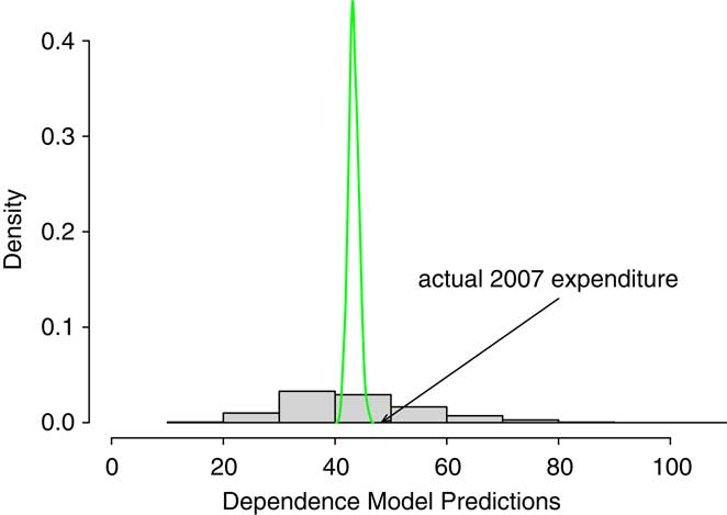
Figure 1 Comparison of Predictive Distributions. The smooth density is the predictive distribution from the independence model. The rectangular histogram is from the dependence model. The arrow marks the actual held-out 2007 expenditures.
Table 12 Out-of-Sample Risk Measures
Table 13 Covariate Description and Percentage of Positive Expenditures by Level of Covariates

Table 14 Marginal Logistic Regressions for Five Types of Events

Table 15 Marginal Regressions for Expenditure of Five Types of Events Assuming Gamma Distribution

Table 16 Out-of-Sample Statistics

In Table 12, we use standard actuarial risk measures, the value at risk, VaR, and conditional tail expectation, CTE, although our approach could be easily extended to other risk measures. The VaR is simply a quantile or percentile, the VaR(α) gives the 100(1 − α) percentile of the distribution. The CTE(α) is the expected value conditional on exceeding the VaR(α). See, for example, Frees et al. (Reference Frees, Shi and Valdez2009) for another predictive modelling application using these risk measures. In Table 12, VaRInd and CTEInd are the value at risk and conditional tail expectation for the independence model whereas VaRDep and CTEDep are the corresponding measures for the dependence model.
As anticipated, both the figure and table show that the predictive distribution for the independence model is much narrower than the model for dependence. In basic probability theory that we teach students, for two random variables X and Y, that  $$$ Var{\rm{(}}X\: + \:Y{\rm{)}}\:{\rm{ = }}\:Var{\rm{(}}X{\rm{)}}\, + \,Var{\rm{(}}Y{\rm{)}}\, + \,{\rm{2}}Cov{\rm{(}}X,Y{\rm{)}} $$$
(here, “Var” is for “variance” and “Cov” is for “covariance”). That is, if X and Y are positively associated, then a model that assumes independence will display less uncertainty than a model that accounts for dependence;
$$$ Var{\rm{(}}X\: + \:Y{\rm{)}}\:{\rm{ = }}\:Var{\rm{(}}X{\rm{)}}\, + \,Var{\rm{(}}Y{\rm{)}}\, + \,{\rm{2}}Cov{\rm{(}}X,Y{\rm{)}} $$$
(here, “Var” is for “variance” and “Cov” is for “covariance”). That is, if X and Y are positively associated, then a model that assumes independence will display less uncertainty than a model that accounts for dependence;  $$$ Var{\rm{(}}X{\rm{)}}\, + \,Var{\rm{(}}Y{\rm{)}}\, \lt \,Var{\rm{(}}X\: + \:Y{\rm{)}} $$$
. In the same vein, Table 12 shows that the model incorporating dependence has a wider spread than the model that ignores these features.
$$$ Var{\rm{(}}X{\rm{)}}\, + \,Var{\rm{(}}Y{\rm{)}}\, \lt \,Var{\rm{(}}X\: + \:Y{\rm{)}} $$$
. In the same vein, Table 12 shows that the model incorporating dependence has a wider spread than the model that ignores these features.
Unfortunately, for our analysis, we have only one held-out realization. Total expenditures in 2007 turned out to be $ 48.34 million. This is unlikely to occur in the model of independence although very plausible in the dependence model. Of course, this does not validate the model of dependence but it is consistent with what we learned from our detailed in-sample analysis.
As a final remark, we note that this sampling procedure was done using the estimated parameters as fixed quantities. An alternative procedure to incorporate their sampling variability into this analysis would be to bootstrap the results.
6 Concluding Remarks
Multivariate two-part regression models can be applied in many different areas of actuarial practice. In this paper, we have cited applications in healthcare, property and casualty (general), and life insurance. Our detailed case study of healthcare expenditures shows that it is important to distinguish between when an event may occur (frequency) and, if it occurs, the amount of expenditure (severity). The explanatory variables that influence an expenditure may differ by whether one is modelling frequency or severity. Moreover, we have found that the association among differ types depends greatly on whether one is modelling frequency or severity.
In this paper, we have used the descriptor “frequency” to describe whether or not an event may occur. We note that there are many important situations in actuarial practice when the analyst has a count of claims and would use a frequency distribution such as a Poisson or negative binomial distribution for modelling. This is also referred to as a “frequency” problem. Clearly, an interesting extension of this paper would be to consider multivariate regression problems where the number of claims for each event type is available.
Acknowledgment
The first author thanks the Assurant Health Insurance Professorship for funding to support this research.
7 Appendix – Additional Survey Details
7.1 Sources of Payment
The total expenditure for medical services is the sum of 12 sources of payment: (1) out-of-pocket by the user or family, (2) Medicare, (3) Medicaid, (4) private insurance, (5) Veterans Administration, excluding TRICARE/CHAMPVA, (6) TRICARE/CHAMPVA, (7) other federal sources including Indian health services, Military treatment facilities, and other care by the Federal government, (8) other state and local sources including community and neighbourhood clinics, state and local health departments, and state programs other than Medicaid, (9) workers’ compensation, (10) other unclassified sources including sources such as automobile, homeowner's, and liability insurance, and other miscellaneous or unknown sources, (11) other private such as any type of private insurance payments reported for persons not reported to have any private health insurance coverage during the year as defined in MEPS, and (12) other public such as Medicare/Medicaid payments reported for persons who were not reported to be enrolled in the Medicare/Medicaid program at any time during the year.
7.2 Zero Expenditures Flat Fee Groups
There are some medical events reported by respondents where the payments were zero. Zero payment events can occur in MEPS for the following reasons:
1. The event was covered under a flat fee arrangement (flat fee payments are included only on the first event covered by the arrangement).
2. There was no charge for a follow-up stay.
3. The provider was never paid by an individual, insurance plan, or other source for services provided.
4. Charges were included in another bill (e.g. for emergency room visits that have a subsequent inpatient stay).
5. The event was paid for through government or privately-funded research or clinical trials.
6. For office-based or outpatient department files that contain events involving a telephone call rather than a medical provider visits, there are no expenditure associated.
7. All expenditures for home health care provided by informal care providers (family, friends, or volunteers) were assigned −1 “inapplicable” because those types of events were skipped out (never asked) of the questions regarding expenditures.
The approach used to count expenditures for flat fee groups was to place the expenditure on the first visit of the flat fee group (stem event). The remaining visits (leaves) have zero facility payments, while physician's expenditures may be still present. Thus, if the first visit in the flat fee group occurred prior to 2006, all of the events that occurred in 2006 will have zero payments. Conversely, if the first event in the flat fee group occurred at the end of 2006, the total expenditure for the entire flat fee group will be on that event, regardless of the number of events it covered after 2006.
There are no flat fee groups regarding prescribed medicine or home health visits. Outpatient and office-based medical provider visits are the only two event types allowed in a single flat fee group. The stem may have been reported as an outpatient department visit and the leaves may have been reported as office-based medical provider visits.
8 Appendix – Odds Ratios
As emphasized in equation (3), odds ratios can be interpreted as conditional odds. This interpretation is particularly convenient when defining higher order associations. We follow standard statistical literature (e.g. Liang et al. Reference Liang, Qaqish and Zeger1992, Section 2) and define higher order association measures in terms of contrasts of conditional odds ratios. Specifically, define the third order association measure
 $${{\zeta }_{{\rm{123}}}}\, = \, {{\zeta }_{{\rm{123}}}}{\rm{(}}{{r}_{\rm{1}}},{{r}_{\rm{2}}},{{r}_{\rm{3}}}{\rm{)}}\, = \, {\rm{ln}}\,{\rm{OR((}}{{r}_{\rm{1}}},{{r}_{\rm{2}}}{\rm{)}}|{{r}_{\rm{3}}}\, = \, {\rm{1) - ln}}\,{\rm{OR((}}{{r}_{\rm{1}}},{{r}_{\rm{2}}}{\rm{)}}|{{r}_3}\, = \, 0{\rm{)}}$$
and the fourth order association measure
 $${ {{\zeta }_{{\rm{1234}}}}\, = \, {{\zeta }_{{\rm{1234}}}}{\rm{(}}{{r}_{\rm{1}}},{{r}_{\rm{2}}},{{r}_{\rm{3}}},{{r}_{\rm{4}}}{\rm{)}} \cr = \, {\rm{ln}}\,{\rm{OR((}}{{r}_{\rm{1}}},{{r}_{\rm{2}}}{\rm{)}}|{{r}_{\rm{3}}}\, = \, {\rm{1}},{{r}_{\rm{4}}}\, = \, {\rm{1)}}\, + \,{\rm{ln}}\,{\rm{OR((}}{{r}_{\rm{1}}},{{r}_{\rm{2}}}{\rm{)}}|{{r}_{\rm{3}}}\, = \, {\rm{0}},{{r}_{\rm{4}}}\, = \, {\rm{0)}} \cr \ {\rm { - ln}}\,{\rm{OR((}}{{r}_{\rm{1}}},{{r}_{\rm{2}}}{\rm{)}}|{{r}_{\rm{3}}}\, = \, {\rm{0}},{{r}_{\rm{4}}}\, = \, {\rm{1) - ln}}\,{\rm{OR((}}{{r}_{\rm{1}}},{{r}_{\rm{2}}}{\rm{)}}|{{r}_{\rm{3}}}\, = \, {\rm{1}},{{r}_{\rm{4}}}\, = \, {\rm{0)}}. \cr}$$
Higher order association parameters are possible (e.g. Liang, et al. Reference Liang, Qaqish and Zeger1992, Section 2) but will not be needed for our application. That is, for our application with p = 5, we assume independence between home health visits and all other events, and set the log odds ratios associated with home health to zero.
Bounds
Knowledge of the marginal means πj and the odds ratios are sufficient to determine joint probabilities and hence evaluate likelihood functions. To illustrate, consider equation (3). Simple algebra shows that
 $$ {\rm{exp(}}{{\zeta }_{{\rm{12}}}}{\rm{)}}\, = \, \frac{{{{\pi }_{{\rm{11}}}}{\rm{(1 \,- \, }}{{\pi }_{\rm{1}}}{\rm{ - }}{{\pi }_{\rm{2}}}\, + \, {{\pi }_{{\rm{11}}}}{\rm{)}}}}{{({{\pi }_{\rm{1}}}\,{\rm{ - }}\,{{\pi }_{{\rm{11}}}}{\rm{)(}}{{\pi }_{\rm{2}}}{\rm \,{ - }}\,{{\pi }_{{\rm{11}}}}{\rm{)}}}}, $$
where  $$$ {{\pi }_{{\rm{11}}}}\: = \:{\rm{Pr}}({{r}_{\rm{1}}}\: = \:{\rm{1}},{{r}_{\rm{2}}}\: = \:{\rm{1)}} $$$
. From this expression, we may determine π 11 as the solution to a quadratic function involving ζ12, π 1, and π 2:
$$$ {{\pi }_{{\rm{11}}}}\: = \:{\rm{Pr}}({{r}_{\rm{1}}}\: = \:{\rm{1}},{{r}_{\rm{2}}}\: = \:{\rm{1)}} $$$
. From this expression, we may determine π 11 as the solution to a quadratic function involving ζ12, π 1, and π 2:
 $${ & {\rm{(exp(}}{{\varsigma }_{12}}{\rm{) - 1)}}\pi _{{{\rm{11}}}}^{{\rm{2}}} {\rm{ - [(exp(}}{{\varsigma }_{{\rm{12}}}}{\rm{) - 1)(}}{{\pi }_{\rm{1}}}\, + \, {{\pi }_{\rm{2}}}{\rm{)}}\, + \, {\rm{1]}}{{\pi }_{{\rm{11}}}}\, \cr & \quad \quad \quad \quad \quad \quad + \, {\rm{exp(}}{{\varsigma }_{{\rm{12}}}}{\rm{)}}{{\pi }_{\rm{1}}}{{\pi }_{\rm{2}}}\, = \, {\rm{0}}. \cr}$$
With this joint probability and marginal means, other joint probabilities  $$$ {\rm{Pr(}}{{r}_{\rm{1}}}\: = \:j,{{r}_{\rm{2}}}\: = \:k{\rm{)}},{\rm{\{ }}j,k{\rm{\} }}\:{\rm{ = }}\:{\rm{\{ 0,1\} }} $$$
may be readily determined.
$$$ {\rm{Pr(}}{{r}_{\rm{1}}}\: = \:j,{{r}_{\rm{2}}}\: = \:k{\rm{)}},{\rm{\{ }}j,k{\rm{\} }}\:{\rm{ = }}\:{\rm{\{ 0,1\} }} $$$
may be readily determined.
Knowledge of third order association parameters ζ123, together with marginal means πj, j = 1,2,3 and joint probabilities Pr(r 1 = j, r 2 = k) allows one to determine joint probabilities of the form  $$$ {\rm{Pr(}}{{r}_{\rm{1}}}\: = \:j,{{r}_{\rm{2}}}\: = \:k,{{r}_{\rm{3}}}\: = \:l{\rm{)}},\;\,{\rm{for}}\,{\rm{\{ }}j,k,l{\rm{\} }}\,{\rm{in}}\,{\rm{\{ 0,1\} }} $$$
. The triple joint probabilities are the solution of a fourth order polynomial equation. Similarly, quadruple probabilities can be found as the solution of an eighth-order degree polynomial.
$$$ {\rm{Pr(}}{{r}_{\rm{1}}}\: = \:j,{{r}_{\rm{2}}}\: = \:k,{{r}_{\rm{3}}}\: = \:l{\rm{)}},\;\,{\rm{for}}\,{\rm{\{ }}j,k,l{\rm{\} }}\,{\rm{in}}\,{\rm{\{ 0,1\} }} $$$
. The triple joint probabilities are the solution of a fourth order polynomial equation. Similarly, quadruple probabilities can be found as the solution of an eighth-order degree polynomial.
There are two difficulties in determining the joint probabilities from knowledge of the marginal means and association parameters. The first is a computational one. Solutions to second, fourth and eighth-order degree polynomials must be found for each observation for each evaluation of the likelihood function. This means that even for data sets that are moderately sized (about 19,000 observations for our application), computational concerns arise. Second, joint probabilities are bounded by lower-order joint probabilities. For example, it is easy to see that
 $${\rm{max(0}},{{\pi }_{\rm{1}}}\, + \, {{\pi }_{\rm{2}}}{\rm{ - 1)}}\,\leq \,{{\pi }_{{\rm{11}}}}\,\leq \,{\rm{min(}}{{\pi }_{\rm{1}}},{{\pi }_{\rm{2}}}{\rm{)}}.$$
Because of this, when we compute the solutions to high-order polynomials for each observation, the roots depend heavily on the specification of the association parameters.
Equation (7) implies that the bounds for bivariate dependence ratio are
 $$\frac{{{\rm{max(}}0,{{\pi }_{\rm{1}}}\, + \, {{\pi }_{\rm{2}}}{\rm{ - 1)}}}}{{{{\pi }_{\rm{1}}}{{\pi }_{\rm{2}}}}}\,\leq \,{{\tau }_{{\rm{12}}}}\,\leq \,{\rm{\Big(}}\frac{{\rm{1}}}{{{{\pi }_{\rm{1}}}}},\frac{{\rm{1}}}{{{{\pi }_{\rm{2}}}}}{\rm{\Big)}},$$
Recall that with dependence ratio approach, it is customary to define a constant dependence ratio over observations. When marginal probabilities are small, the dependence ratio approach works well since equation (8) could be easily satisfied by a constant dependence ratio. For high-frequency events, e.g. office-based visits, the marginal probability is high and equation (8) leads to very strict restrictions on the constant dependence ratio. Care must be taken to set appropriate boundaries for dependence ratio in the modelling algorithm.
With odds ratio approach, it is customary to define a constant odds ratio over observations. While the odds ratio is constant, the dependence ratio varies over observations. This allows one to apply the approach even when the marginal probabilities are relatively large. Taking exp( $$$\varsigma$$$
12)→0, it is easy to solve for π 11 from equation (6):
$$$\varsigma$$$
12)→0, it is easy to solve for π 11 from equation (6):
 $${{\pi }_{{\rm{11}}}}\, = \, \frac{{{{\pi }_{\rm{1}}}\, + \, {{\pi }_{\rm{2}}}{\rm{ - 1}}\, + \,|{{\pi }_{\rm{1}}}\, + \,{{\pi }_{\rm{2}}}{\rm{ - 1}}|}}{{\rm{2}}}\, = \,{\rm{max(0}},{{\pi }_{\rm{1}}}\, + \, {{\pi }_{\rm{2}}}{\rm{ - 1)}}.$$
Taking exp( $$$\varsigma$$$
12)→∞, it is easy to see that
$$$\varsigma$$$
12)→∞, it is easy to see that
 $${{\pi }_{{\rm{11}}}}\, = \, \frac{{{{\pi }_{\rm{1}}}\, + \, {{\pi }_{\rm{2}}}{\rm{ - }}|{{\pi }_{\rm{1}}}{\rm{ - }}{{\pi }_{\rm{2}}}|}}{{\rm{2}}}\, = \, {\rm{min(}}{{\pi }_{\rm{1}}},{{\pi }_{\rm{2}}}{\rm{)}}.$$
Hence, a mild constraint on the odds ratio, i.e., exp( $$$\varsigma$$$
12) > 0 would make equation (7) satisfied even if the marginal probabilities are relatively large. In this sense, given a fixed association parameter over observations, the odds ratio approach is preferred to the dependence ratio approach when the outcomes of interest contain one or more frequent events.
$$$\varsigma$$$
12) > 0 would make equation (7) satisfied even if the marginal probabilities are relatively large. In this sense, given a fixed association parameter over observations, the odds ratio approach is preferred to the dependence ratio approach when the outcomes of interest contain one or more frequent events.


