


INTRODUCTION
Marine dissolved organic carbon (DOC) is the oceans’ largest organic carbon reservoir. Ultraviolet photochemical oxidation (UVox) has been used for decades as a method to measure DOC concentrations (noted herein as [DOC]), δ13C, and Δ14C values (Armstrong et al. Reference Armstrong, Williams and Strickland1966; Williams Reference Williams1968; Williams et al. Reference Williams, Oeschger and Kinney1969). Renewed interest in DOC has resulted in the development of several custom UVox systems, with commonly sought after methodological improvements that include higher sample throughput (>1× sample per day), smaller C blanks, and smaller sample volumes (Beaupré et al. Reference Beaupré, Druffel and Griffin2007; Xue et al. Reference Xue, Ge and Wang2015). DOC Δ14C values measured on systems that reproducibly achieve blank-corrected yields of standards within uncertainty of 100%, δ13C and Δ14C values within uncertainty of consensus values, and methodological precisions less than natural DOC variability are required to reliably interpret marine DOC biogeochemistry. Therefore, careful, continual examination of all procedures from sample collection to isotopic blank corrections are essential for accurate, reproducible, and intercomparable DOC Δ14C measurements performed on each UVox system. In order to minimize uncertainties, parameters including UVox reactor kinetics, trapping efficiencies, manometric precisions, and blank corrections should be characterized routinely (Beaupré et al. Reference Beaupré, Druffel and Griffin2007). Here, we highlight additional parameters to consider when collecting and preparing samples for UVox. We also share several recent “hurdles” we have encountered as important considerations improving UVox efficiency, quantitative sample C recovery, decreasing carbon blanks and minimizing potential isotopic fractionation within UVox systems.
METHODS
UV Photochemical Oxidation at UC Irvine
Marine DOC samples are collected by filtering seawater from Niskin bottles through pre-combusted (540°C, 2 hr) GF/F filters (0.7 µm) held in acid cleaned (10% HCl) 70 mm stainless steel filter holders fitted with acid cleaned platinum cured silicone tubing. All GF/F filters are pre-combusted in individual Al foil “envelopes” to minimize C contamination during sample collection. The filtered seawater is collected in pre-combusted (540°C, 2 hr) 1-L amber Boston round bottles. Each bottle is rinsed 3 times with 100 mL of sample prior to filling with ∼800 mL of seawater, and then sealed with a Teflon lined cap. An additional layer of chromic acid cleaned PTFE tape is placed between the cap and bottle. Samples are immediately frozen at sea in a 20°C chest freezer, at a 15–20° angle to prevent bottle breakage during freezing.
For detailed discussion of most DOC line run parameters, including a diagram of our vacuum line and reactor systems, we refer the reader to Beaupré et al. (Reference Beaupré, Druffel and Griffin2007). We routinely use the dilution method for UVox isolation of DOC from seawater (Beaupré et al. Reference Beaupré, Druffel and Griffin2007; Griffin et al. Reference Griffin, Beaupré and Druffel2010; Druffel et al. Reference Druffel, Griffin and Walker2013; Walker et al. Reference Walker, Griffin and Druffel2016). Here, seawater DOC samples (∼800 mL) are diluted to ∼1000 mL with 18.2 MΩ cm Milli-Q water (MQ; 0.4–1.0 μM C) prior to UVox. There are several advantages in using the dilution method. First, it effectively reduces the detection limit of a DOC line instrument to very small volumes of seawater (30 mL) (Beaupré et al. Reference Beaupré, Druffel and Griffin2007). Second, this method saves time by eliminating the need to pre-irradiate MQ water to be used as diluent for samples and standards. It also reduces the total number of standards that are needed for AMS corrections, and thus preparation time from two days to one day (Griffin et al. Reference Griffin, Beaupré and Druffel2010). Third, dilution allows for routine monitoring of MQ blank C and DOC system line blanks that can be directly used to correct sample concentrations and isotopic values via mass balance. Finally, it prevents evaporative loss of seawater and a buildup of salts on the reactor wall closest to the lamp—preventing a decrease in UVox efficiency.
During sample loading, diluent and sample water volumes are determined non-intrusively by measuring the meniscus height from outside the quartz reactor using a homemade, calibrated cathetometer. The cathetometer is comprised of a 30 cm ruler fixed vertically, and level in both x and y, to a laboratory ring stand. Reactor meniscus heights are read using a 3× power hand lens to an accuracy of 0.5 mm. Reactor-specific volume (mL) and meniscus height (cm) relationships are experimentally determined by measuring known aliquots of MQ water by mass and applying a least squares linear regression analysis. MQ water density is also inferred using a linear density approximation (0.9982 g/mL at 20°C, 0.9957 g/mL at 30°C) after measuring its temperature. The resultant linear regression is then used to determine daily sample and diluent volumes based on their meniscus heights with propagated uncertainties of ±3–5 mL.
After loading, the sample is then acidified with 1 mL 85% phosphoric acid (Fisher HPLC grade). Dissolved inorganic carbon (DIC) is sparged from the sample using ultra high purity (UHP; 5.0) He gas. The mixing ratio of CO2 venting from the sample is monitored with an infrared gas analyzer (LiCOR, LI-6252) and logged to a lab computer. The LiCOR is calibrated bi-monthly with standard reference gases (0–500 ppm CO2 in He). Following complete DIC removal, DOC samples are UV oxidized to CO2 using a 1200W medium-pressure mercury arc lamp for 4 hr. The CO2 produced photochemically from DOC is then sparged with UHP He, purified cryogenically, and manometrically quantified. At all stages, UHP He flow rates are quantified with a 50 mL soap-film bubble flow meter (Restek, #RES-20136) at the LiCOR’s vent.
Following manometry, equilibrated gas splits of CO2 are taken for Fm and δ13C measurements at UCI’s Keck Carbon Cycle AMS (KCCAMS) Laboratory. One split (2–800 µgC) is graphitized via sealed-tube Zn reduction (Xu et al. Reference Xu, Trumbore, Zheng, Southon, McDuffee, Luttgen and Liu2007; Walker and Xu Reference Walker and Xu2019) for accelerator mass spectrometry radiocarbon (AMS 14C) measurements. The other split is cryogenically transferred to 3 mm diameter, 5.5 cm length, Pyrex tubes for δ13C analysis with a Gas Bench II and Finnigan Delta Plus IRMS (Walker et al. Reference Walker, Druffel, Kolasinski, Roberts, Xu and Rosenheim2017). Consensus values for isotopic standards are either known (e.g. from IAEA) or experimentally determined via elemental analysis and IRMS (EA-IRMS; ±0.1‰).
The total reproducibility of these methods for [DOC], Fm, and δ13C values are [DOC] ±1.3μM, Fm ±0.004, and δ13C ±0.2‰, respectively (Walker et al. Reference Walker, Griffin and Druffel2016). However, in some cases we have observed Fm of ±0.010 when seawater samples were split in half and analyzed after long storage periods (Druffel et al. Reference Druffel, Griffin and Walker2013). The system “line” blank (i.e. re-irradiated MQ water) ranges from 3 to 12 µgC, but is typically ∼4 µgC.
RESULTS AND DISCUSSION
Collection, Storage, and Preparation of Seawater DOC Samples
Extreme care should be taken during DOC sample collection, storage, and laboratory preparation to minimize any possible extraneous C addition. Previous work has shown that acidification and room temperature storage of filtered seawater results in loss of semi-labile (14C modern) DOC (Walker et al. Reference Walker, Griffin and Druffel2016). While frozen storage does not appear to be affected, it is prone to the unpredictable precipitation of salt crystals that can introduce [DOC] and isotopic measurement errors (Beaupré and Druffel Reference Beaupré and Druffel2009). For example, Druffel et al. (Reference Druffel, Griffin and Walker2013) noted changes in DOC recovery (by 1–5 µM), Δ14C offsets (±10‰, or Fm ±0.0100), and δ13C bias (–0.3‰) for duplicate aliquots of seawater from the same sample bottles that were measured on different days. Thus, phase transitions and inconsistent transfer of sample carbon from storage bottles to the UVox reactor may lead to measurement artifacts (Beaupré and Druffel Reference Beaupré and Druffel2009).
In order to minimize errors associated with frozen storage, we originally restricted our measurements to samples that did not develop visible crystals (Beaupré and Druffel Reference Beaupré and Druffel2009). To increase the proportion of useable samples, Walker et al. (Reference Walker, Griffin and Druffel2016) quantitatively transferred the contents of each sample bottle into the reactor via rinsing to achieve reproducibility in [DOC], Fm, and δ13C of ±1.3 µM, ±0.0094, and ±0.1‰, respectively. Since these crystals are likely precipitated carbonates (Beaupré et al. 2009), we now acidify and shake thawing samples in their storage bottles to re-dissolve crystals before transferring seawater to the reactor (Figure 1). The acidified seawater and any remaining crystals are then transferred quantitatively to the reactor with three or four ∼50 mL MQ rinses. These simple procedures have provided reliable storage, compositional fidelity, and decreased variability in [DOC], Δ14C (or Fm) values (Griffin et al. unpublished data).
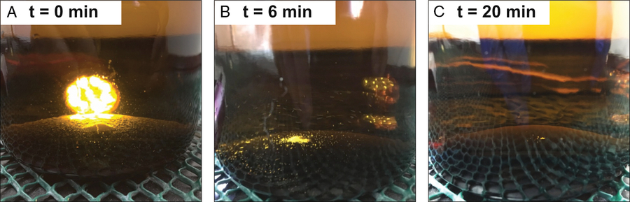
Figure 1 Dissolution of crystals from thawed seawater samples. Pictured is a time series of a thawed, acidified sample with abundant crystals. The sample was vigorously shaken every 1 min to achieve crystal re-dissolution. (A) 1.0 mL of phosphoric acid is added to the 1-L amber Boston round sample bottle, a flashlight behind the bottle helps illustrate the mound of crystals. (B) Half of the original crystals remain after 6 min of repeated shaking. (C) Almost 100% of crystals have re-dissolved by 20 min of shaking.
Liquid Nitrogen Trap Efficiency and Minimizing Break Through (BT)
The DOC line at UC Irvine utilizes two highly efficient compact Horibe traps to cryogenically trap water (−78°C, dry ice and isopropanol slush) and sample CO2 (–196°C, liquid nitrogen; LN2) (Beaupré et al. Reference Beaupré, Druffel and Griffin2007). In early tests of the DOC line, He streams with high CO2 mixing ratios and flow rates were found to allow some sample CO2 to “break through” (BT) the LN2 Horibe trap and leave the system without being quantified. CO2 BT was experimentally determined to be minimized through an initial reduction in He flow rate (to below 50 mL min–1) during the sparging of sample DOC. However, data from these experiments were never published and unfortunately, the procedure of reducing the DOC initial sparge rate, was never adopted as standard lab practice. Thus, throughout much of the DOC line’s history (2008–2017), BT was present and some sample C was lost from our DOC samples. An example of a LiCOR trace during a full day experiment is shown in Figure 2 and illustrates this C BT during the DOC sparge step. We have conducted a series of experiments, seeking to quantify and minimize C BT.
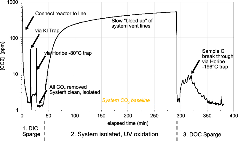
Figure 2 Example of monitoring CO2 gas leaving the DOC UVox line over an experiment. At the beginning of the day, DIC and residual CO2 in the DOC line is removed via acidification of the sample and sparging with UHP He (DIC Sparge). When all residual CO2 is removed, the He flow is stopped, the line isolated from atmosphere and UVox started. Throughout UVox, the system vent tubing slowly “bleeds up” to lab air. This does not affect the DOC sample, because it is isolated. After 4 hr, the UVox is stopped and He gas is used to sparge all resultant CO2 for isolation in the Horibe trap (DOC Sparge). In this example, a flow rate of 200 mL min–1 was used. Several minutes later, we see sample C breaking through the Horibe trap and leaving the system (0–10 ppm). BT lasts between 45 and 70 min, depending on [DOC] and flow rate.
Quantifying BT as a Function of [DOC] and Flow Rate
We analyzed 8 OX-I standards to determine the amount of BT as a function of [DOC] in the reactor, and the flow rate of He gas during the DOC sparge. First, BT was measured at two flow rates of He (200 mL min–1 and 250 mL min–1) during the DOC sparge, at [DOC] values ranging from 20 to 75µM. Results show that BT at both flow rates are equal (22±2 µgC) for samples with [DOC] values of 12 and 15µM (Figure 3A). However, for samples with higher [DOC] values (>30 µM), BT is consistently higher for samples that were sparged at 250 mL min–1 than those sparged at 200 mL min–1. The average of three BT values for tests run at 200 mL min–1 is 27.3±2.9 µgC, and that for tests run at 250 mL min–1 is 34.9±0.4 µgC. We observe no significant differences between Fraction Modern (Fm) values of samples run at the different He flow rates or [DOC] values (Figure 3B). Stable C isotopic (δ13C) results also show no significant differences in the samples (Figure 3C). In this limited dataset, we do not observe fractionation of carbon isotopes with changing [DOC] or He flow rate.

Figure 3 Mass and C isotopic effects of sample breakthrough (BT) at differing OX-I [DOC] and flow rates. (a) relationship between mass of BT as CO2 (µgC) at two He flow rates and three [DOC] values. (b) DOC OX-I Fm values, both uncorrected and corrected, showing no effect of sample BT C on corrected 14C measurements. (c) uncorrected DOC OX-I δ13C values show no isotopic fractionation with sample C BT. In plots B and C, the green line represents the consensus Fm and δ13C value of OX-I. (Please see electronic version for color figures.)
Following these findings, we have made corrections to our [DOC] values for samples to account for the lost CO2 (BT) run at UC Irvine prior to these tests; this has resulted in a 3–4 µM increase in our [DOC] values. In addition, we have adopted the practice of DOC sparging at a He flow rate of 45–54 mL min–1. This practice has minimized our DOC sample C BT to <3 µgC for samples and isotopic standards (200–700 µgC), and 0.5 to 1.0 µgC for MQ blanks (10–15 µgC) and line blanks (typically ∼4 µgC). By adopting these changes (i.e. adding C lost via BT and subtracting the line blank), we routinely achieve DOC standard yields of 100±2%.
Testing of New Stainless Steel Cryogenic Trap Designs
Following the discovery of Horibe trap C BT, we developed and tested several new cryogenic trap designs. One hypothesis for the observed C BT is that as sample CO2 builds up at the LN2 interface of the glass Horibe trap wall, it may reach a critical mass or geometric shape that permits CO2 “snow” to blow away, sublimate and leave the system with the flowing He gas. One economical solution to this problem was to build a stainless steel trap containing many loops, forcing sample CO2 to pass through multiple LN2 and room temperature interfaces. Stainless steel has the added benefits of being easy to work with and a much higher thermal conductivity (16 W m–1 K–1) than glass (1 W m–1 K–1) (Lide Reference Lide2005), and thus should be more efficient at trapping CO2. We have tested three types of stainless steel cryogenic traps for sample C BT.
The first trap was made from 0.25 inch OD 304 stainless steel tubing (3.5 m length, ID = 5.3 mm) wrapped to form 7 loops ∼6 inches in height. The trap was adapted to the DOC line with Swagelok Ultra-Torr fittings and vacuum tested. Only the bottom third of the trap was placed in LN2, thus forcing sample CO2 to cross a total of 14 thermal interfaces between room temperature (20°C) and LN2 (–196°C). This trap was tested via acidification of bicarbonate (DOC = 800 µM) in MQ and He stripping at 200 mL min–1 to simulate a DOC sample (as above in the section Quantifying Break Through (BT) as a Function of [DOC] and Flow Rate). In this test, we quantified 70±7 µgC BT in the first hour of sparging. A second test (DOC = 800 µM) of this trap with 6-mm Pyrex rods installed, to force sample gas onto the side walls of the trap, yielded a nearly identical amount of C BT (78±7 µgC).
We tested a second trap design made from 0.125 inch OD 304 stainless tubing (3.6 m in length, ID = 1.4 mm) with a total of 8 loops and 16 thermal interfaces. In our first bicarbonate (DOC = 800 µM acidification/sparge test, the trap clogged within the first 5 min of the experiment, likely due to the small tubing diameter, high CO2 trapping efficiency and the large mass of C being sparged. We observed zero C BT during this experiment.
A third, hybrid trap design, was tested where sparged CO2 was first passed through the 0.25 in trap, and next via the 0.125 in trap coupled with a Swagelok Ultra-Torr fitting. This trap had a path length of 7.1 m, a volume of 84 mL and a combined total of 15 loops and 30 thermal interfaces (Figure 4A,B). Instead of using bicarbonate acidification, we performed two tests with a standard reference gas (400 ppm CO2 in UHP He) at 150 mL min–1 and 50 mL min–1. These tests resulted in similar rates of C BT (0.020 µgC min–1) at both flow rates (Figure 4C,D). Once new baseline values were reached for the reference gas flowing through the LN2 trap, we determined a total C BT mass of 2.08±0.21 and 2.30±0.23 µgC at the low and high flow rate condition through integrating 10 minutes of baseline, respectively. Rates of C BT were slightly higher than the glass Horibe trap at 50 mL min–1 (0.001 µgC min–1). Since our modified trap designs did not appear to yield better results, we currently recommend using a glass Horibe trap (design specified in Beaupré et al. Reference Beaupré, Druffel and Griffin2007), at a DOC sparge flow rate of 50 mL min–1 to minimize C BT. In the future, we intend to test copper tubing traps, which are more affordable, and have a much higher thermal conductance (∼400 W m–1 K–1) (Lide Reference Lide2005).

Figure 4 Hybrid stainless steel cryogenic trap design and C BT results. (A) Side-view of the hybrid 0.25 in and 0.125 in OD stainless cryotrap next to a 15 cm ruler. (B) View of hybrid stainless trap in use. The bottom third of the cryotrap is placed in liquid nitrogen (LN2) allowing CO2 gas to heat up and re-freeze on each pass around the trap. (C) LiCOR trace of CO2 (ppm; black line) and rate of CO2 loss (µgC min–1; green line) exiting the system as CO2 (400 ppm) in He reference gas is flowed at 150 mL min–1. (D) LiCOR trace of CO2 (ppm; black line) and rate of CO2 loss (µgC min–1; green line) exiting the system as CO2 (400 ppm) in He reference gas is flowed at 50 mL min–1. Plots C and D, the blue line represents the baseline CO2 ppm value achieved with pure UHP He (no CO2) prior to the beginning of the experiment. Black arrows indicate the moment liquid nitrogen (LN2) was added to the trap, at which point the resultant LiCOR CO2 ppm values decrease. Grey shaded regions show the 10 min integration periods, from which equilibrated trap BT CO2 ppm values were determined.
DOC Line Extraneous C Sources and Use of Standards for Blank Corrections
There are two methods for determination of extraneous C blanks and correction of 14C data in a DOC UVox system (Figure 5). The first is the direct method, where extraneous C blank masses and Fm values are experimentally measured and then these C contributions subtracted from sample measurements via isotopic mass balance. With the direct method, it is imperative that this isotopic mass balance include propagation of known measurement uncertainties for both samples and extraneous C blanks. The second method is the indirect method where extraneous C blanks are quantified indirectly by measuring small to ultra-small sizes of both 14C-free and modern standard reference materials. The 14C-free standards are used to determine masses of extraneous modern carbon (MC; Fm = 1) contributions, and modern standards (OX-1) for extraneous dead carbon (DC; Fm = 0) contributions. These DC contributions are also commonly referred to as C backgrounds. The indirect method and mass balance equations are clearly presented in Santos et al. (Reference Santos, Southon, Griffin, Beaupré and Druffel2007). With the indirect method, ±50% uncertainty for both MC and DC mass contributions are prescribed as a precaution.
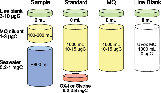
Figure 5 Conceptual diagram of carbon mass contributions and aqueous volumes for DOC samples, standards, diluent and line blanks. Various amounts of extraneous C are added for each sample type and diluent volume used. A ubiquitous, volume-less extraneous carbon “line blank” is inherent to all DOC UVox measurements. A seawater sample prepared using the dilution method also contains 100–200 mL of low carbon Milli-Q water as a diluent. A DOC isotopic standard (0.2–0.8 mgC) is accurately weighed and quantitatively transferred to the reactor with diluent. Standards contain far more MQ diluent by both mass (10–15 µgC) and aqueous volume (1000 mL) than samples. A diluent blank (MQ) is comprised only of MQ carbon and the line blank.
Both the direct and indirect methods have their own advantages and disadvantages for DOC data. For example, the indirect method does not inherently require routine monitoring of MQ diluent or line blank C masses or Fm values (albeit we strongly recommend users do this). The indirect method also does not require ultra-small mass graphitization, which can be difficult for many labs to achieve and measure on an AMS. However, there are a few disadvantages to the indirect method for DOC line data: (1) it requires analysis of many analytical “process” isotopic standards (ideally 3× for MC and 3× for DC varying in size between 50 and 500 µgC) in order to accurately determine Fm blank contributions, (2) standards are not fully representative of sample matrix (for seawater), and also overestimate MQ C (10–15 µgC) contributions to samples containing <3 µgC (MQ), and (3) this method does not adequately control for the presence of a ubiquitous DOC system line blank.
There are many reasons users should move towards the direct method of blank correction, because it: (1) can be more easily implemented given recent advances in ultra-small mass (2–25 µgC), sealed tube Zn graphitization (Walker and Xu Reference Walker and Xu2019), (2) does not overestimate C contributions from MQ diluent, (3) can effectively correct for ubiquitous system line blanks underlying all UVox measurements, (4) yields more representative [DOC] and isotopic values with propagated uncertainties, and (5) can be applied with sample matrix matching (i.e. the addition of pre-combusted salt to seawater standards and blanks), which should control for possible UVox fractionation due to halides in solution. We note that, in the case of UVox systems, the direct method requires frequent analysis of both MQ diluent and line blanks to constrain blank Fm variability. This variability can be a function of changes in user operation, system parameters, MQ [DOC], and extraneous organic C sources, such as upstream CO2 sorbents (e.g. Ascarite II), and the KI trap solution.
Direct measurement of ultra-small DOC line blanks and diluents has historically precluded the implementation of the direct method for UVox systems. At UC Irvine, the vast majority of our samples have been corrected using the indirect method. Recently, our group has started implementing direct method corrections through quantification of MQ diluent and DOC line blank Fm values using the ultra-small mass sealed tube Zn method (Walker and Xu Reference Walker and Xu2019). In the case of DOC line blanks, the validity of a 0 µgC contribution from re-irradiated MQ (RIMQ) ultimately depends on the handling/storage of this re-irradiated MQ to prevent addition of extraneous C. We measure MQ and RIMQ on sequential UVox days, keeping the RIMQ in the quartz reactor overnight, in order to minimize contamination of the line blank. We routinely measure both modern and 14C-free isotopic standards (OX-I and Glycine, respectively), with a MQ, line blank, or isotopic standard run approximately every 6–8 samples (bi-weekly). We note that salt is currently not added to the diluent used for our isotopic standards. This may affect indirect-method blank corrections as standards in a saline matrix may behave differently than in fresh water during UVox would likely have a different extraneous C blank.
Historical Record of DOC UVox Isotopic Standard Fm Values at UC Irvine
Corrected Fm and Δ14C values are typically reported for DOC samples. However, to date only a handful of studies have reported percent yields and 14C values of standard reference materials run on DOC UVox systems (Beaupré et al. Reference Beaupré, Druffel and Griffin2007; Griffin et al. Reference Griffin, Beaupré and Druffel2010; Beaupré and Druffel Reference Beaupré and Druffel2012; Druffel et al. Reference Druffel, Griffin and Walker2013). Since the establishment of the DOC UVox method at UC Irvine, we have measured over 170 isotopic standards for the correction of [DOC] and Fm values. A summary of corrected and uncorrected Fm values for these isotopic standards is shown in Figure 6. Note that DOC standards run in 2017–2018 were blank corrected using the direct method.
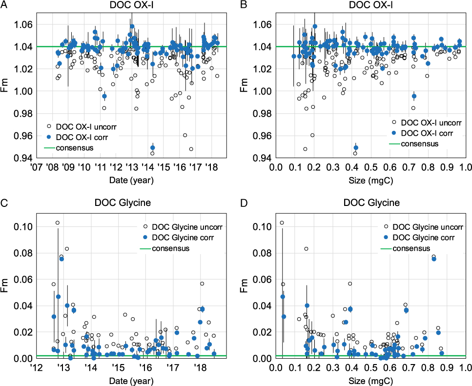
Figure 6 Fraction modern (Fm) values of DOC isotopic standards at UC Irvine. (A) DOC OX-I Fm values (n = 109) vs. date of UVox, (B) DOC OX-I Fm values vs. size, (C) DOC Glycine Fm values vs. date of UVox, (D) DOC Glycine Fm values (n = 67) vs. size. In all plots, open and closed symbols represent uncorrected and blank corrected Fm data, respectively. Green lines indicate OX-I and Glycine consensus Fm values. Error bars represent 1-sigma propagated errors of blank corrected Fm values.
Over the past decade, the majority of our measured DOC OX-I standard Fm values are correctable within 2-sigma of the consensus OX-I value (Fm = 1.0398). DOC OX-I corrected with the direct method (2017–2018) are less variable and more accurate (closer to the consensus OX-I Fm value). This suggests an improved dead C blank correction over the indirect method (i.e. less extraneous MQ C is subtracted from samples). While propagated uncertainties increase with decreasing DOC OX-I sample size, Fm values remain correctable within 2-sigma propagated error of the consensus OX-I Fm value (Figure 6B). Overall, our 14C-free DOC Glycine Fm values (2012–present) are more variable (Figure 6C,D), suggesting DOC samples are more susceptible to modern extraneous C contributions. Of the few DOC Glycine samples we have measured in 2017–2018, the indirect method also slightly under-corrects for modern C contamination. We typically achieve a combusted Glycine Fm value <0.0020 at UC Irvine, however many corrected DOC Glycine’s have Fm values >0.0050. Aside from larger propagated uncertainties with smaller standard sizes, there does not appear to be a trend between corrected DOC Glycine Fm values and sample size (Figure 6D).
In order to evaluate the difference between direct vs. indirect blank corrections on DOC Fm values, we use a Bland-Altman (difference) plot on a dataset of n = 34 DOC samples in which both corrections were applied (Figure 7). The coefficient of determination of least squares regression is weak (R2 = 0.26), however it is statistically significant, with slope errors excluding zero (m = 0.0012±0.0004). These results show that modern samples (Fm = 1.0) are less affected by the blank correction methods than half-modern (Fm = 0.5) or dead samples (Fm = 0.0). This indicates that the indirect method is over correcting for MQ C contributions (Fm = 0.4–0.7). Direct blank corrected Fm values are lower than indirect corrected value by 0.0021±0.0006 (Δ14 = 2.1±0.6‰). In addition, propagated Fm individual DOC measurement uncertainties with the direct method (Fm ±0.0052‰) are more representative of our true analytical uncertainty (Fm ±0.0040–0.0100, or Δ14C ±4–10‰), than individual measurement errors determined via the indirect method (Fm ± 0.0020).
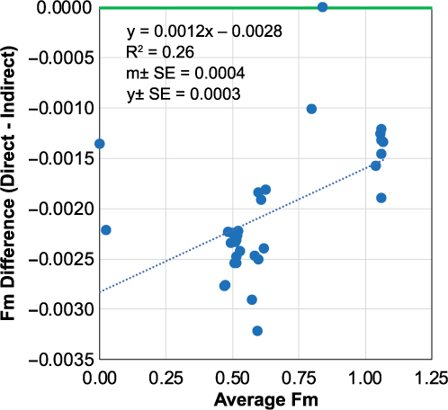
Figure 7 Bland-Altman difference plot illustrating direct and indirect blank corrected DOC sample Fm data. Green line indicates no difference between the two correction methods. The dashed blue line represents the least squares linear regression of the method difference vs. average Fm value of the two methods. Data are from n = 34 DOC sample “unknowns” measured at UC Irvine in March 2018.
Historical Record of DOC UVox Isotopic Standard δ13C Values at UC Irvine
Most UVox studies have focused primarily on [DOC] and 14C measurements. Wide ranges in seawater DOC δ13C values (∼3‰) have been reported from similar depths and locations (e.g. Broek et al. Reference Broek, Walker, Guilderson and McCarthy2017; Zigah et al. Reference Zigah, McNichol, Xu, Johnson, Santinelli, Karl and Repeta2017). Studies seeking to constrain UVox DOC δ13C values have received less attention. Here we discuss the historical record of DOC isotopic standard δ13C values measured at UC Irvine (Figure 8).
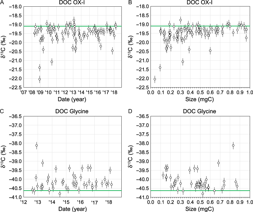
Figure 8 Stable isotopic (δ13C) permil values of DOC isotopic standards at UC Irvine. (A) DOC OX-I δ13C values vs. date of UVox, (B) DOC OX-I δ13C values vs. samples size, (C) DOC Glycine δ13C value vs. date of UVox, (D) DOC Glycine δ13C value vs. sample size. In all plots, open symbols represent uncorrected δ13C values. Green lines indicate consensus δ13C values for OX-I (IAEA reported value) and Glycine (determined at UCI by routine EA-IRMS and closed tube combustion measurements). Error bars represent assigned ±0.2‰ errors of UVox δ13C values.
Since 2008, our DOC OX-I δ13C values have ranged from –18.8‰ to –22.0‰ with an average value of –19.5‰ (±0.5‰ standard deviation, n = 95; Figure 8A). Since 2012, DOC Glycine δ13C values range from –38.1‰ to –40.8‰ with an average value of –40.1‰ (±0.5‰ standard deviation, n = 46; Figure 8C). Prior to October 2013, we did not fully equilibrate DOC CO2 gas splits for δ13C. Instead, sample gas was “bled” off the main sample through a stopcock. We hypothesize that much of the δ13C variability observed for both OX-I and Glycine (average δ13C = –19.6±0.6‰, n = 55 and –40.0±0.9‰, n = 9, before October 2013, respectively) can be attributed to mass-dependent isotopic fractionation induced by this process. Small samples would display a higher degree of mass-dependent fractionation (Figure 8B,D).
After October 2013, we began fully equilibrating CO2 gas splits by expanding into a larger volume with a 2 min equilibration time prior to “splitting” for 13C (∼12–35 µgC), (∼300–500 µgC) and an archive (100 µgC). With gas equilibration, DOC OX-I and Glycine values are less variable and more accurate, with δ13C values 0.1‰ closer to consensus values (–19.5±0.2‰, n = 40 and –40.1±0.4, n = 37, respectively). While our recent BT tests did not reveal apparent δ13C fractionation (see above in section Quantifying BT as a Function of [DOC] and Flow Rate), excluding n = 1 OX-I and Glycine outliers, over the past year our δ13C accuracy has overall improved and our variability decreased after controlling for C BT (–19.3±0.1‰, n = 13 and –40.2±0.1‰, n = 7). Currently, our isotopic standards are within 0.2‰ and 0.4‰ of consensus δ13C values for OX-I and Glycine, respectively. October 2013, we have prescribed 1-sigma ±0.2‰ DOC δ13C errors to help bracket these offsets.
DOC OX-I δ13C values are almost always equal to or lower than consensus EA-IRMS values (–19.1±0.1‰), whereas DOC Glycine’s are almost always higher than consensus EA-IRMS values (–40.6±0.1‰). Possible explanations for these offsets include (1) varying contributions of extraneous C blanks from addition of MQ water as a diluent, (2) intra-molecular isotopic heterogeneity of 13C/12C ratios (e.g. the amino-C vs. carboxyl-C groups in Glycine have different δ13C values), and (3) the UVox process induces C-isotope fractionation differentially for these two compounds. While we have not tested the latter two processes, we believe MQ and extraneous C blank contributions could largely explain our observed offsets (i.e. in both Fm and δ13C). We are currently working towards examining these effects more closely. For example, we have recently measured δ13C of our MQ diluent to be –26‰ (Walker et al. unpublished data). Thus, MQ C contributions to DOC standards would make DOC OX-I δ13C more negative and DOC Glycine more positive than their canonical values. The δ13C value of OX-I is ∼7‰ different from that of MQ and Glycine is ∼14.6‰ different from that of MQ. Given the mass contribution of MQ C to DOC standards and these isotopic endmember offsets, DOC Glycine values should therefore be more affected by blank C contributions than OX-I. This is consistent with our observed offsets of DOC standards from consensus values (Δδ13C=–0.2‰ and +0.4‰ for OX-I and Glycine, respectively). Small DOC standards should be more affected by MQ C contributions, because they comprise a larger relative percent mass of the DOC standard. However, we do not currently have enough data to make this comparison. Finally, we still working towards determining the best method for DOC δ13C blank correction. In the interim, our lab reports “uncorrected” DOC δ13C values with prescribed 1-sigma errors of ±0.2‰.
UVox Community and Methodological Recommendations
Based on our experience, we have several methodological recommendations for consideration by the broader UVox community. These are especially important for users developing their own homebuilt systems, or using adapted commercial UVox systems (e.g. Ace Glass #7900). First, effectively parameterize the UVox efficiency and kinetics of the system. Particular attention should be paid to the system lamp geometry, power, and photon flux reaching the reactor. In addition, reactor design, sample homogenization (via stirring), cooling and vacuum line design are important considerations. For detailed discussion of these parameters, we refer the reader to Armstrong et al. (Reference Armstrong, Williams and Strickland1966), Beaupré et al. (Reference Beaupré, Druffel and Griffin2007), and Oppenländer (Reference Oppenländer2007).
For sample preparation and UVox analysis, we recommend care to minimize contamination and maximize procedural efficiency and consistency. Samples should be filtered using pre-combusted GF/F filters (0.7 µm) and stored frozen, as opposed to acidified at room temperature (Walker et al. Reference Walker, Griffin and Druffel2016). When loading samples into the reactor, it is imperative that all crystals (if present) be loaded into the reactor by rinsing with MQ diluent prior to UVox. The presence of crystals precludes the loading of partial samples from a single bottle into the reactor. A low [DOC] diluent should be used (e.g. Milli-Q) and its C content measured regularly for proper correction of [DOC] and isotopic values. Any CO2 leaving the UVox system, including that which breaks through the LN2 trap during DOC sparge, should be quantified and used to correct reported [DOC] data. This step requires the use of a sensitive CO2 analyzer (0–400 ppm range).
We recommend routine analysis of diluent blanks, line blanks and isotopic standards, such that quantitative (100%) yields of standards and samples can be ensured and appropriate direct or indirect corrections can be made to DOC Δ14C values. At UC Irvine, we typically measure the following standards and blanks interspersed between sets of six DOC samples; a MQ diluent and subsequent DOC line blank (RIMQ) the following day, a large DOC OX-1 (500 µgC), a small DOC Glycine (200 µgC), another set of MQ diluent/line blanks, a small DOC OX-I (200 µgC) and a large DOC Glycine (500 µgC).
For the radiocarbon community, we recommend that UVox users report at a minimum: AMS lab numbers, [DOC], Fm or Δ14C of samples, standards (with % yields) and blanks, the year of collection, year of measurement, and IRMS determined δ13C values (if AMS 13C values are measured, state this but do not report values). In addition, propagated [DOC] and isotopic uncertainties must be determined and reported. With many new UVox systems coming online, the need for a community-wide inter-comparison study is apparent. UVox measurements should result in quantitative yields (i.e. 100%), after blank and BT corrections are applied and errors propagated. A UVox system producing low yields will fractionate DOC based on its inherent photochemical lability. Here, a UVox measurement will not be representative of total DOC, nor directly comparable with measurements from other UVox systems. Publishing standard yields and isotopic data will help users assess the inter-comparability of results—thus helping to shape future interpretations of DOC cycling in the environment.
ACKNOWLEDGMENTS
We acknowledge Noreen Garcia for help with graphitization, and general laboratory assistance. Jennifer Walker, Dachun Zhang and Xiaomei Xu aided with δ13C analysis at UC Irvine. Sample Fm values were determined by us at the UC Irvine W. M. Keck Carbon Cycle Accelerator Mass Spectrometry Laboratory. We thank John Southon for his advice and help with AMS analysis. This work was funded by NSF Chemical Oceanography program (OCE-141458941 to E.R.M.D., and OCE-1536597 to S.R.B.) and an American Chemical Society Petroleum Research Fund New Directions (PRF-55430-ND2) Grant (to B.D.W. and E.R.M.D.).


