


1. Introduction
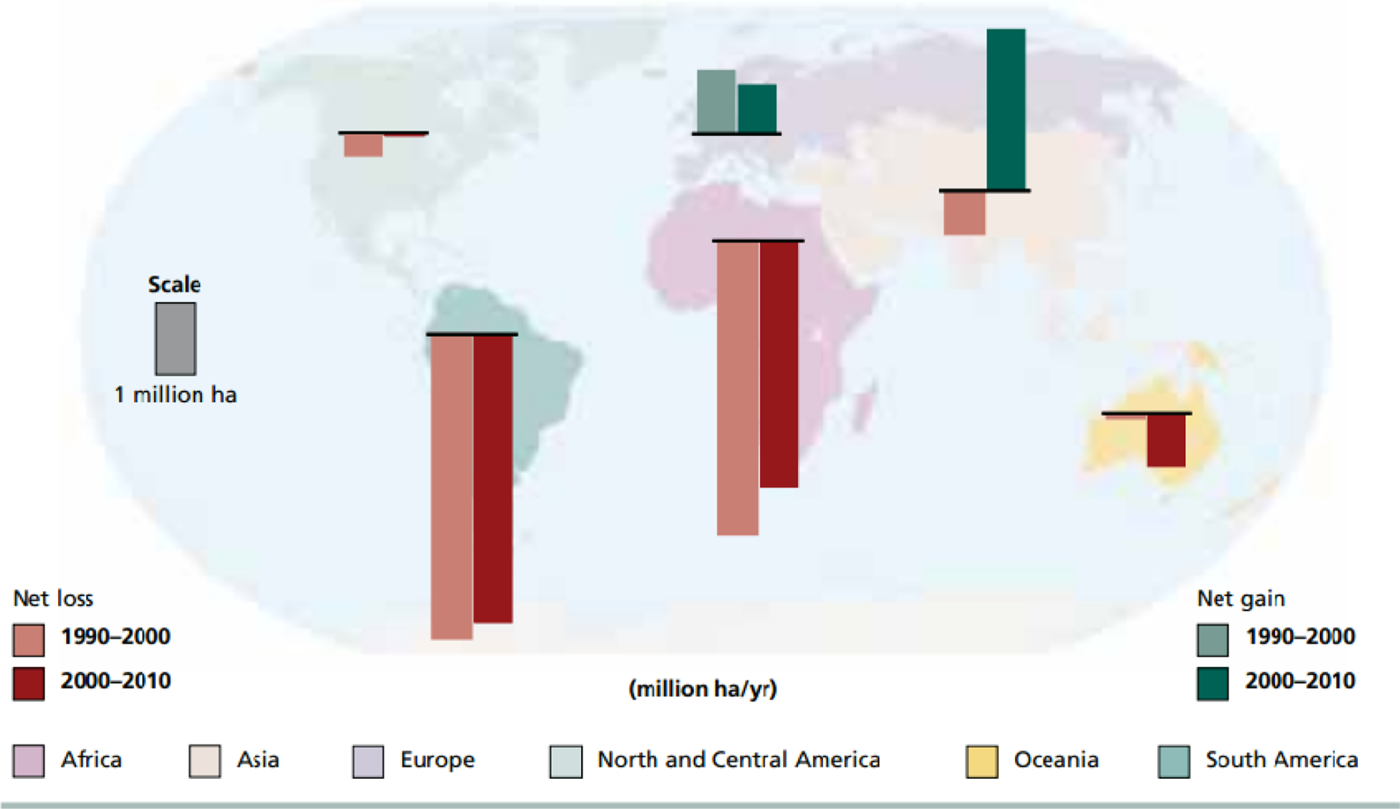
Deforestation continues to be a major environmental issue in tropical developing countries. According to the Food and Agriculture Organization (FAO, 2010), deforestation is still rising in Latin America and Africa. These two continents recorded an annual loss of about 4 and 3.4 million hectares respectively between 2000 and 2010. This has both environmental and social consequences.
At the environmental level, deforestation causes the destruction of biodiversity and ecosystem services such as soil stabilization, conservation of water, controlling erosion and desertification (FAO, 2010). Deforestation also contributes to global warming because it is a major source of CO2 emissions, contributing about 17–18 per cent of global greenhouse gas emissions per year (IPCC, 2007; WRI, 2008). At the social level, deforestation reduces the livelihood resilience and thereby increases the poverty of forest-dependent people. Indeed, deforestation increases the risk of vulnerability to economic and environmental shocks faced by the local poor population (FAO, 2010).
The importance of forest degradation in tropical developing countries can be explained by the fact that these countries are at the beginning of their development process which requires strong growth and expansion of income to address the problem of poverty. Forest degradation leads to an increased demand for agricultural and forestry products in which countries have a comparative advantage (Culas, Reference Culas2007). This trend is unlikely in developed countries where demand is directed to the environmental services. This situation is characterized in the literature as the inverted-U shape relationship between income growth and environmental quality (Grossman and Krueger, Reference Grossman and Krueger1995), more commonly known as the environmental Kuznets curve (EKC).
Theoretically, López (Reference López1994) explains the appearance of the EKC for deforestation by internalization of the effects of the stock of forest resources on agricultural production. Indeed, he shows that when there are feedback effects from the stock of forest resources – that is, the change in the stock of forest resources affects production – economic growth in developing countries tends to decrease the degradation of these resources if individual producers or the State internalize these stock effects. This implies that when producers ignore the shadow value of forest resources in their decisions, an increase in production (economic growth) is accompanied by a rise in deforestation. But when producers have incentives to increase the stock (internalize the stock feedback effects) because the scarcity of resources has negatives effects on production, the deforestation rate tends to decrease, taking a Kuznets inverted-U shape.
Another explanation for the EKC for deforestation may rely on changes in the labor market and the ability of government to protect forest resources. First, the high wage rates in non-agricultural sectors can attract agricultural workers to migrate to other areas. This has the effect of reducing the pressure on forests and reducing the rate of deforestation. Second, government policy – through the strengthening of forest institutions – can contribute to the enforcement of forest protection (Culas, Reference Culas2007).
Several empirical studies have attempted to validate the EKC hypothesis for deforestation in the countries of Latin America, Africa and Asia (Cropper and Griffiths, Reference Cropper and Griffiths1994; Koop and Tole, Reference Koop and Tole1999; Bhattarai and Hammig, Reference Bhattarai and Hammig2001; Culas, Reference Culas2007). However, these studies may suffer from econometric weaknesses including the spurious regression problems associated with the presence of unit roots (Wagner, Reference Wagner2008) and the identification of time effects issue (Vollebergh et al., Reference Vollebergh, Melenberg and Dijkgraaf2009), insofar as these studies are based on the traditional approach of analyzing the variables as levels.
To circumvent these weaknesses, Stern et al. (Reference Stern, Gerlagh and Burke2017) have proposed a new approach in terms of the long-run growth rate. The advantage of this approach is that it allows us to analyze the EKC and convergence hypotheses in a unified framework and directly test the relative explanatory power of each. The convergence hypothesis is a theoretical alternative to the EKC that analyzes the income–environmental degradation relationship in terms of convergence. Developed by Brock and Taylor (Reference Brock and Taylor2010), the convergence approach extends the Solow growth model (Reference Solow1956) by incorporating environmental concerns. This approach shows that countries converge in terms of pollution emissions. Specifically, if countries share the same economic parameter values – such as savings rate, pollution intensity, rate of technical progress – but different initial conditions, they will tend to converge in terms of the extent of their pollution (Brock and Taylor, Reference Brock and Taylor2010).
Similarly, from a neoclassical growth model with endogenous emission reduction, Ordas Criado et al. (Reference Ordas Criado, Valente and Stengos2011) have predicted a beta-convergence in pollution. They explained the existence of convergence effects on the one hand by globalization that leads to economic structures and the technologies used across countries becoming more similar over time and, on the other hand, by to the fact that emission-intensive countries are taking policy measures to improve their environment and/or reduce their dependence on energy imports. Empirical studies have found evidence of the convergence effects on pollutants focusing on CO2 and SO2 (Aldy, Reference Aldy2006; Westerlund and Basher, Reference Westerlund and Basher2008; Brock and Taylor, Reference Brock and Taylor2010; Ordas Criado et al., Reference Ordas Criado, Valente and Stengos2011; Herrerias, Reference Herrerias2013; Stern et al., Reference Stern, Gerlagh and Burke2017).
Although the theoretical and empirical literature analyzing the convergence hypothesis has focused on environmental degradation related to air pollution, it is important to note that forces explaining the existence of convergence effects in emissions – such as economic globalization and the implementation of environmental policies by countries in order to improve their environment and tackle climate change – are also crucial in understanding changes in forest cover. Indeed, studies have shown that economic globalization has indirectly led to the improvement of forest resources in some tropical developing countries. This is due, on the one hand, to the remittances that have enabled some households to stop working in the fields in favor of service activities (Hecht and Saatchi, Reference Hecht and Saatchi2007) and, on the other hand, to improving the structure of exports by absorbing FDI in the manufacturing and service sectors to develop export-oriented manufacturing and service industries (Li et al., Reference Li, Liu, Long, de Jong and Youn2017).
It has also led to the imposition of common environmental protection rules in all countries, which has had a negative impact on deforestation. For example, the implementation of international initiatives to reduce CO2 emissions from deforestation and forest degradation (REDD+)Footnote 1 ultimately contributes to the preservation of forest cover in tropical developing countries. Nevertheless, globalization through global markets has also negatively affected forest cover. Some studies have found a positive correlation between forest loss and trade of agricultural and forestry products in tropical developing countries (DeFries et al., Reference DeFries, Rudel, Uriarte and Hansen2010; Kastner et al., Reference Kastner, Erb and Nonhebel2011; Henders et al., Reference Henders, Persson and Kastner2015).
Given that forces explaining the existence of convergence effects in pollution are also drivers for changes in forest cover, it is appropriate ask whether convergence effects may be a determinant in understanding forest cover change in tropical developing countries. This is all the more relevant in that recent studies have shown that some tropical developing countries are undergoing a forest transition, that is, a positive change in their forest cover over time. For example, this situation has been observed in India, Bangladesh, Costa Rica (Kanninen et al., Reference Kanninen, Murdiyarso, Seymour, Angelsen, Wunder and German2007), China (Xu et al., Reference Xu, Yang, Fox and Yang2007) and Viet Nam (Mather, Reference Mather2007).
However, the structural, economy-wide factors such as government policy, technological change and demography – which are key drivers of forest changes – are ignored in the literature on the forest transition theory (Barbier et al., Reference Barbier, Burgess and Grainger2010). Therefore, the convergence hypothesis based on these factors would be appropriate to analyze the changes in forest cover across countries. Thus, the objective of this paper is to test whether convergence effects are as important as income effects in explaining changes in forest cover.
The contribution of this study relative to the existing literature on the EKC for deforestation is to analyze the deforestation–income relationship by using the new approach in order to show that convergence effects are also important in explaining changes in forest cover. Results show that the EKC is not significant. However, there is a beta convergence across developing countries in terms of deforestation per capita. In other words, these countries converge in terms of policies that prevent deforestation and forest degradation. This implies that, just as with growth effects, beta convergence effects are also important in explaining changes in forest cover in tropical developing countries.
This paper is organized as follows. Section 2 is a review of the literature on the income–environmental degradation relationship. Section 3 discusses the methodological issues and section 4 presents the data. The results are presented in section 5 and section 6 concludes the study.
2. The relationship between economic development and environmental degradation
The literature on the link between economic development and environmental degradation focuses on two theoretical approaches. The first relates to the traditional theory based on the EKC hypothesis which postulates that the relationship between several indicators of environmental degradation and income exhibits an inverted-U shape. The second is more recent and is considered to be an alternative to the EKC hypothesis (Stern, Reference Stern2014). It is based on the convergence hypothesis which argues that countries will converge in terms of emissions (Brock and Taylor, Reference Brock and Taylor2010). In other words, environmental degradation will first increase in poor countries with high economic growth rates before fading when these countries catch up with the rich countries.
2.1 EKC hypothesis
The EKC hypothesis was first explained by the combination of three types of effects that occur in the development process: (i) the production scale effect, which means that the increase in production is accompanied by pollution; (ii) the composition effect, which takes into account the pollution intensity levels of different industries, and (iii) the technological effect, which describes technology changes in the production process (Grossman and Krueger, Reference Grossman and Krueger1991, Reference Grossman and Krueger1995; Panayotou, Reference Panayotou1993). Theoretical models then began to be developed. According to de Bruyn and Heintz (Reference de Bruyn, Heintz and van den Bergh2002) and Kijima et al. (Reference Kijima, Nishide and Ohyama2010), the theoretical mechanisms underlying these models are based on three factors: changes in behavior and preferences, institutional changes, and technological and organizational changes.
In the case of deforestation, the theoretical explanation of the EKC is provided by López (Reference López1994). He considers an economy with two sectors: a primary sector that uses natural resources as a factor of production, and the rest of the economy that uses other factors. The primary sector is characterized by agriculture whose production is dependent not only on the cultivated land area (the level of deforestation) but also on the forest stock ensuring quality and soil fertility. He found that when the effects of stock of forest resources on agricultural production are internalized, the economic growth in developing countries will be accompanied by low deforestation along the trajectory of the inverted U-shape. A number of empirical studies have attempted to validate or invalidate the Kuznets relationship between different indicators of environmental degradation and income in the last two decades. In general, the mixed results are due either to the type of environmental indicators used in the country or the group of countries studied; the explanatory variables used; the period of time considered; and econometric techniques used (Bhattarai and Hammig, Reference Bhattarai and Hammig2001).
The first empirical studies on deforestation began in the 1990s with the studies of Cropper and Griffiths (Reference Cropper and Griffiths1994), Shafik (Reference Shafik1994) and Koop and Tole (Reference Koop and Tole1999). The findings of these studies are different despite their having used the same quadratic model. But these findings may be explained by differences in sample and study period. Indeed, Cropper and Griffiths (Reference Cropper and Griffiths1994), based on panel data from 64 countries from 1961 to 1988, found that the EKC is verified in Africa and Latin America but not in Asia. Koop and Tole (Reference Koop and Tole1999), however, show that the EKC only exists in the countries of Latin America when using panel data from 76 tropical developing countries from 1961 to 1992. In contrast, Shafik (Reference Shafik1994) finds no evidence of the existence of the EKC from a sample of 66 countries over the period 1962–1988.
Apart from the differences in the samples, studies during the first decade did not take into account institutional factors in their analysis. Yet institutional development plays an important role in the environmental degradation and economic growth relationship. Indeed, institutional factors affect the EKC relationship, especially in low-income countries. For example, the level of education, political freedoms and civil rights can help to improve the quality of the environment (Torras and Boyce, Reference Torras and Boyce1998). Similarly, the quality of public policies such as security of property rights or better enforcement of contracts can help flatten the EKC and reduce the environmental cost of economic growth (Panayotou, Reference Panayotou1997).
This gap was filled by the research work during the second decade whose major difference was a focus on institutional indicators. Thus, Bhattarai and Hammig (Reference Bhattarai and Hammig2001), by incorporating institutional variables, confirm the EKC relationship for 66 countries in Latin America and Africa but find no evidence in Asia from 1971 to 1991. They also show that institutional indicators (political rights and civil liberties) significantly reduce deforestation. Similarly, Ehrhardt-Martinez et al. (Reference Ehrhardt-Martinez, Crenshaw and Jenkins2002) show the existence of an EKC with a threshold of US$1,150 in 74 least-developed countries over the period 1980–1995. They also find a negative effect of the strengthening of democracy on deforestation. Culas (Reference Culas2007), using the quality indicators of environmental policy such as the implementation capacity of the contracts and the efficiency of the bureaucracy, finds an EKC relationship for deforestation only for Latin American countries. He confirms the positive effect of improving institutional policies on reducing deforestation over the period 1972–1994.
However, some studies have rejected the existence of the EKC despite controlling institutional factors. In particular, Barbier (Reference Barbier2004), in contrast to previous studies, used as the dependent variable the expansion of agricultural land which is a proxy for deforestation. Using a quadratic model, he finds no evidence of the existence of the EKC in samples from Latin America, Asia and Africa over the period 1961–1994. Concerning institutional variables, Barbier shows that corruption control reduces the expansion of agricultural land and thus negatively affects deforestation. Similarly, Arcand et al. (Reference Arcand, Guillaumont and Jeanneney2008) developed a theoretical model focusing on the factors affecting the incentives to transform the forested land into agricultural land. By testing these theoretical hypotheses on a sample of 101 countries from 1961 to 1988, they find that the EKC is not valid. However the authors show that stronger institutions reduce deforestation.
Furthermore, other studies have questioned the supposed parametric form of the relationship between deforestation and income. The purpose of this work is to explore a possible nonlinearity in the process of deforestation. Thus, Azomahou and Van (Reference Azomahou and Van2007), from a nonparametric approach, reject the EKC relationship between income and deforestation for 59 developing countries. However, they find the same results on the institutions, while Chiu (Reference Chiu2012), using a threshold effect panel model, shows that the EKC is verified for 52 developing countries during the period 1972–2003. This approach allows him to determine the endogenous turning point as between US$2,459–3,021.
2.2 Convergence hypothesis
The convergence hypothesis is a new approach to understanding the relationship between the environment and economic growth. This hypothesis was theoretically enhanced by the work of Brock and Taylor (Reference Brock and Taylor2010) based on the stylized facts. These authors were inspired by Solow's (Reference Solow1956) growth model and support the idea that the forces of diminishing returns and technical progress, identified by Solow as being fundamental to the growth process, may also be in the growth–environment relationship. Thus, Brock and Taylor (Reference Brock and Taylor2010) extend the Solow model by assuming that production generates pollution and a constant share of production is allocated to clean-up activities through technical change abatement.
Results show that countries converge in terms of emissions. In other words, emissions increase initially in poor countries because of their rapid growth, but they decrease later when growth slows (due to the forces of convergence to the developed countries' stationary state). These results imply that the mechanism that governs emissions is the decline in production growth rate that is induced by convergence forces combined with the constant rate of technical progress in the abatement of pollution. However, Stefanski (Reference Stefanski2013) shows that the emissions path of developing countries can also be determined by changes in the growth rate of the emission intensity due to structural changes in these economies.
Moreover, Ordas Criado et al. (Reference Ordas Criado, Valente and Stengos2011), using a neoclassical growth model with endogenous emission reduction, have predicted a beta-convergence in pollution. However, unlike Brock and Taylor (Reference Brock and Taylor2010), they assume that both the saving rate and the propensity to spend on abatement are endogenously determined by utility maximization. Also, their framework is considered to be a flow-pollution model in which emission-reducing investment is excluded and a clean-technologies model where abatement is optimized without capital accumulation. This allows them to derive the joint dynamics relationship between pollution growth, pollution levels, and income growth rates, which can be tested using regression methods.
In the case of deforestation, it is a convergence in terms of deforestation which is consistent with the forest transition hypothesis (Mather, Reference Mather1992). According to Mather, forest cover tends to decrease in countries which are at the beginning of their development and this trend is reversed in developed countries with an increase in forest cover through reforestation. This change in forest cover is what the author called forest transition – that is, the passage from deforestation to reforestation. Nevertheless, according to recent studies, this transition can also be observed in developing countries through the awareness of climate change issues and the implementation of emission reduction instruments caused by deforestation and forest degradation (REDD+). For example, this phenomenon is observed in India, Bangladesh, Costa Rica (Kanninen et al., Reference Kanninen, Murdiyarso, Seymour, Angelsen, Wunder and German2007), China (Xu et al., Reference Xu, Yang, Fox and Yang2007) and Viet Nam (Mather, Reference Mather2007).
In the literature, there are three types of convergence. The first is beta convergence which means that poor countries tend to grow faster (and are therefore more polluting) than rich countries (Sala-i-Martin, Reference Sala-i-Martin1996). Technically, it is indicated by an inverse relationship between the growth of a variable and its initial level (Barro and Sala-i-Martin, Reference Barro and Sala-i-Martin1992). The second, sigma convergence, is defined as a convergence which occurs if the dispersion of the current level of per capita GDP of a group of countries tends to decrease over time (Sala-i-Martin, Reference Sala-i-Martin1996). This implies in the case of pollution or deforestation that countries will have on average approximately the same levels of future emissions or deforestation. The third is stochastic convergence which states that a pair of countries converges stochastically if their differences are stationary emissions (Aldy, Reference Aldy2006).
The convergence hypothesis has been empirically tested by many studies. These tests have largely focused on CO2 emissions and results differ according to the type of convergence, study sample, and methods used. Thus, Strazicich and List (Reference Strazicich and List2003) show from the tests of both cross-section data regression (beta-convergence) and unit root (stochastic convergence) that 21 industrialized countries converge on CO2 emissions over the period 1960–1997. Aldy (Reference Aldy2006) confirms these previous results by the sigma-convergence tests for 23 OECD countries, unlike the full sample of 88 countries that diverge on CO2 emissions per capita over the period 1960–2000. Moreover, Westerlund and Basher (Reference Westerlund and Basher2008), using a unit root test on a panel of 28 countries (developed and developing) covering the period 1870–2002, show that these countries converge in CO2 emissions. In contrast, over the period 1870–2009, Herrerias (Reference Herrerias2013) finds only a convergence club of CO2 emissions by energy source for many countries. By empirically testing their theoretical hypothesis of absolute convergence in per capita emissions arising from the Green Solow model, Brock and Taylor (Reference Brock and Taylor2010) find a convergence of CO2 per capita for 165 developed and developing countries between 1960 and 1998.
Finally, to circumvent econometric weaknesses suffered by the analysis of level variables in the EKC, Stern et al. (Reference Stern, Gerlagh and Burke2017) use an approach in terms of the long-term growth rate of the emissions and income relationship. These econometric weaknesses relate in particular to unit root problems (Wagner, Reference Wagner2008) and indeterminacy of the temporal effect (Vollebergh et al., Reference Vollebergh, Melenberg and Dijkgraaf2009). Stern et al.'s (Reference Stern, Gerlagh and Burke2017) approach allows them to test both the EKC and the beta convergence hypotheses of the Green Solow model. They find an EKC for emissions of both SO2 and CO2, which however has a turning point out of sample. The authors also confirm the beta convergence for the two pollutants over the period 1971–2010 on a sample of 134 developed and developing countries.
3. Empirical analysis
3.1 Empirical model
The empirical model is inspired by the new approach developed by Stern et al. (Reference Stern, Gerlagh and Burke2017). This approach is based on the long-run growth rate of the environmental degradation indicator and income. The advantage of the long-run growth rate method compared to the traditional approach of analyzing variables as levels is that it allows us first to test several theoretical hypotheses including both the income-environmental degradation elasticity, and the EKC and convergence hypotheses. Then, by taking the average growth rate over a long period of time, it allows us to filter short-run effects and to put more weight on the long-run components of variability. Finally, this approach solves a number of econometric problems such as spurious regression and time effect identification. It is therefore suitable for analyzing the dynamics of the rate of change of forest cover that is assumed to be non-stationary (Polomé and Trotignon, Reference Polomé and Trotignon2016).
The empirical form is given by:

where ${\hat{F}_i}$ is the long-run rate of change of forest cover per capita (called deforestation if this rate is negative) defined by ${\hat{F}_i} = (1/T)({{F_{iT}} - {F_{i0}}} )$
 where FiT and Fi 0 are the log of the per capita forest area at the end of period T and the early period of country i respectively. ${\hat{G}_i}$
 is the long-run growth rate of GDP per capita of country i : ${\hat{G}_i} = (1/T)({{G_{iT}} - {G_{i0}}} )$
 where GiT and Gi 0 are the log of per capita GDP in the last period and the country's early period respectively. X is a vector of control variables including the agricultural land (as a percentage of land area), the population density (number of people per hectare), the degree of openness, the literacy rate, and institutions (political rights and civil freedoms). These variables are averages over the period studied with the simple cross-country mean deducted.
In equation (1), α 1 represents income-deforestation elasticity which is expected to be positive in accordance with the IPAT (Impact = Population × Affluence × Technology) hypothesis, and α 0 is an estimate of the mean of ${\hat{F}_i}$ for countries with zero economic growth, with the others variables being constant. As the sample mean is deducted from each of the continuous levels variables, α 0 may be interpreted as the mean rate of change in forest cover for a country. β 1 is the coefficient associated with the interaction variable between the rate of economic growth and the initial level of the log per capita income to test the EKC deforestation hypothesis. The latter is verified if α 1 > 0 and β 1 < 0. The EKC turning point can be computed where $\partial \hat{F}/\partial \hat{G} = 0$
 as $\tau = exp ({ - ({\alpha_1}/{\beta_1}) + {\mu_G}} )$
 , where μG is the cross-country mean of initial GDP per capita that was deducted from the initial level of the GDP per capita variable prior to estimation. The convergence hypothesis, in turn, holds if β 2 < 0, that is, there is beta convergence in the level of forest per capita (see Barro and Sala-i-Martin, Reference Barro and Sala-i-Martin1992). Likewise if β 3 = −β 2, then there is beta convergence in the initial forest area per dollars $({\tilde{F}_{i0}} = {F_{i0}} - {G_{i0}})$
 without an additional effect of the initial level of income on the change in growth rate of forest cover.
Moreover, to capture the impact of the level of income on the time effect, equation (1) is estimated by replacing Gi 0 with Gi (the log of income per capita averaged over time in each country). Hence, if β 3 > 0, then forest cover use (or deforestation) declines faster over time, the higher the level of income (holding the others variables constant). This would be consistent with the positive (resp. negative) correlation between forest cover changes (resp. forest cover use) and income per capita.
Following Stern et al. (Reference Stern, Gerlagh and Burke2017), other empirical specifications are tested by applying restrictions to equation (1). These exclusion restrictions are tested using likelihood ratio tests. First, the Ordas Criado et al. (Reference Ordas Criado, Valente and Stengos2011) model is tested by setting β 1 = 0, which is given as follows:

One would expect α 1 > 0 (in the case of deforestation) and β 2 < 0. This means that the change in growth rates of forest cover is positively related to output growth (scale effect) and negatively related to forest cover level (called a defensive effect according to Ordas Criado et al. (Reference Ordas Criado, Valente and Stengos2011)).
Second, the short-run Green Solow model (Brock and Taylor, Reference Brock and Taylor2010) is tested by setting ${\alpha _1} = {\beta _1} = {\beta _3} = 0$ :
:

According to Brock and Taylor, the beta-convergence holds if β 2 < 0.
We also set β 1 = β 3 to derive a basic EKC model in growth rates without the initial per capita forest cover and income terms:

One would expect α 1 > 0 and β 1 < 0 for all negative values of ${\hat{F}_i}$ in the case of deforestation.
Finally, a simple IPAT-inspired growth rates model is tested by setting ${\beta _1} = {\beta _2} = {\beta _3} = 0$ :
:

One would expect α 1 = 1, consistent with a simple IPAT model which assumes that technology is held constant. Otherwise α 1 < 1, which would mean that technology influences the rate of economic growth (Ehrlich and Holdren, Reference Ehrlich and Holdren1971).
3.2 Identification strategy
Models are estimated by OLS with the White robust standard error to correct the problem of heteroscedasticity. Indeed, it is likely that the variance of the error term is inversely related to the explanatory variables or related to the effect of the group. This not only because of the fact that the variables of interest (deforestation and GDP per capita) are averages over the sample size, but it can also exist in the sample group (Stern et al., Reference Stern, Gerlagh and Burke2017). The White (Reference White1980), Breusch and Pagan (Reference Breusch and Pagan1979) and Harvey (Reference Harvey1976) tests are used to check all forms of heteroscedasticity. One first uses the White test for the general form of heteroscedasticity. The Breusch-Pagan test is then used for the form in which the model residuals' variance varies with a set of regressors. Finally, it is possible that the residual variance is related multiplicatively with regressors, which leads us to use the Harvey test.
It is also likely that there is an endogeneity problem related to a potential feedback effect of the GDP growth rate and the average GDP level on the rate of deforestation. This feedback goes through agricultural production and forest resources since the agricultural sector and forest resources contribute to income in developing countries. Therefore, deforestation can have an impact on the GDP growth rate. To solve this omitted variable bias, control variables are introduced, such as the level of agricultural production and the degree of openness that influence both the GDP growth rate and the rate of deforestation.
4. Data
4.1 Description of variables
This study focuses on tropical developing countries which are of interest because deforestation is one of the major environmental problems in these countries (see figure 1). The sample consists of 34 African countries, 21 Latin American countries, 12 Asian countries and 18 European countries (see table Α2 in online appendix 2). The countries were chosen based on the importance of their forest area and its changes. Data on variables cover the period from 1990 to 2010 (for data sources, see table A1 in online appendix 1).
4.1.1 Deforestation rate
Deforestation is defined as the net annual change in forest area (FAO, 2010). In other words, it is the negative variation of annual forest cover. Thus, the deforestation rate is the percentage annual decrease in forest area, that is, the percentage decrease in annual forest cover (Culas, Reference Culas2007). In this study, the long-run deforestation rate per capita is captured by the negative sign of the long-run rate of change in forest cover per capita, defined as the percentage change in the area per capita at the beginning and the end of the period. This variable has been divided by the population size to minimize the bias that may occur when population is large relative to the available forest resources. This may also be relevant in that it captures natural wealth per capita in terms of resource availability for the entire population.
4.1.2 Explanatory variables
Several factors are responsible for deforestation. In this research, we use the relevant macroeconomic and institutional variables in the literature based on available data. All these variables are averages over the study period.
Long-run growth rate of GDP per capita: Theoretical results show that the long-run relationship between environmental degradation (e.g., deforestation, emissions) and income is nonlinear and takes a Kuznets, inverted-U shape. This is justified for several reasons, especially the fact that environmental quality is a luxury good (McConnell, Reference McConnell1997; Lieb, Reference Lieb2002). Indeed, in the first stage of growth, the income-emission elasticity is low (lower than unit), and then it becomes high (greater than one) when the income level is important for financing pollution control activities. Therefore, a potential Kuznets curve implies that the income-environmental degradation elasticity is significantly different from zero or at least below the unit. An EKC occurs when the coefficient associated with the quadratic income term is negative, indicating a technical change effect (Stern et al., Reference Stern, Gerlagh and Burke2017).
GDP per capita: Income per capita plays an important role in the preservation of forest resources. Certainly, it is possible that a high level of income stimulates demand for non-forest products. But the demand for agricultural and forestry products is higher in countries with predominantly agricultural production and low per capita income. Indeed, the level of deforestation is very high in countries with low income per capita and tends to be negative in countries with high income per capita because developed countries record high afforestation and reforestation rates (FAO, 2010). The introduction of the average per capita GDP into the model allows us to interpret the constant as the annual change in deforestation rate of a country with average log income and zero growth rate (Anjum et al., Reference Anjum, Burke, Gerlagh and Stern2014). GDP per capita is measured in purchasing power parity (US$, 2005).
Initial level of forest area: The initial area is used to test the beta convergence hypothesis in terms of deforestation. This hypothesis assumes that there is a negative relationship between the growth rate of a variable and its initial value (Barro and Sala-i-Martin, Reference Barro and Sala-i-Martin1992). Thus, the rate of change in the percentage of forest area should be negatively related to the initial area. Therefore, the deforestation rate would tend to increase with the level of the initial area. This means that countries with high deforestation rates converge to countries with low deforestation rates, assuming that these countries share the same economic parameters values (Brock and Taylor, Reference Brock and Taylor2010).
Agricultural land (percentage of land area): The agricultural sector is the main cause of deforestation in developing countries because of its significant contribution to income, employment and exports (FAO, 2010). This is justified by the practice of extensive agriculture that increases the share of arable land area in these countries. This tends to increase deforestation, which remains the only way to increase agricultural production and income (Culas, Reference Culas2007). However, the effect can be reversed or attenuated when agriculture is intensive. To capture the pressure exerted by the agricultural sector on the forest, we use the definition of agricultural land given by FAO. That is, the share of land area that is arable, under permanent crops, and under permanent pastures in the country during the year.
Population density: Demographic pressures affect the quality of the environment. An increase in the population, therefore, puts pressure on demand for forest products and agricultural land, causing deforestation. An increase in population can also cause pressure in the labor market, leading to a rise in unemployment which may have a negative effect on the forest (Culas, Reference Culas2007). However, population growth may reduce the deforestation rate through income growth and technological progress (Cropper and Griffiths, Reference Cropper and Griffiths1994). Indeed, the increase in income may modify demand for other sources of energy such as firewood. The adoption of technical progress in agriculture can reduce the pressure on the forest through the practice of intensive agriculture.
Degree of openness: International trade influences the quality of the environmental. Indeed, trade affects production and consumption structures of countries that have an effect on the quality of the environment (Sheldon, Reference Sheldon2006). Thus, trade liberalization can play a significant role in the environmental quality of a country. According to the standard Heckscher-Ohlin, countries' participation in trade is based on their factor endowments. Rich countries which have abundant capital will produce capital-intensive goods. In contrast, poor countries with abundant natural resources and labor will specialize in the production of goods that are intensive in natural resources. This may worsen the problem of the tragedy of the commons facing natural resources in general and forest resources in particular in poor countries. In this study, the degree of openness is used to capture the effect of trade, including the trade of agricultural and forest products, on deforestation.
Institutional variables: Institutions play an important role in environmental protection, either by funding clean-up activities or by clearly defining property rights. Thus, the quality of the environment is only the result of the interaction between pollution and pollution control that is ensured by authorities' regulation (Panayotou, Reference Panayotou1997). Empirically, studies have shown an adverse effect of institutional policies on deforestation (Bhattarai and Hammig, Reference Bhattarai and Hammig2001; Culas, Reference Culas2007). Most of these studies use civil liberties, institutional variables, and political rights. Indeed, Dasgupta and Mäler (Reference Dasgupta, Mäler, Behrman and Srinivasan1995) argue that the link between environmental protection and political rights and civil liberties is very close. Following Azomahou and Van (Reference Azomahou and Van2007), the two variables – civil liberties and political rights – are aggregated to form an institutional policy indicator which varies between 2 and 14, to avoid a possible correlation between both variables. The higher the value of the indicator, the lower the quality of the institutions.
Literacy rate: Education is a key factor in environmental protection. It changes the environmental preferences of economic agents and increases demand for environmental quality. Indeed, education allows agents to have more access to information about the harmful effects of environmental degradation (consequences of deforestation) and can, therefore, change their behavior (Bimonte, Reference Bimonte2002). Moreover, according to Farzin and Bond (Reference Farzin and Bond2006), an educated population is more receptive to environmental protection measures implemented by regulators to improve environmental quality. The authors showed that there is a negative correlation between the rate of illiteracy and environmental policy measures. The literacy rate of the adult population seems more relevant in the case of deforestation and allows us to compare our results with those of the existing literature.
4.2 Descriptive statistics
Table 1 reports the descriptive statistics. It shows that the average rate of long-run forest cover change per capita is negative (−0.0181) which is indicative of deforestation. Deforestation is more important in the African countries than in other developing countries. Indeed, the average rate of long-run forest cover change per capita is −0.03 in Africa versus −0.01 in the non-African sample (see tables A3 and A4 in online appendix 3). However, the positive maximum value (0.0266) means that some countries are in the process of reforestation. The average rate of long-run growth of income per capita is positive (0.020), and its smallest and highest values are, respectively, −0.0323 and 0.211. This might explain the forest cover degradation due to the scale effect of the economic activity (Grossman and Krueger, Reference Grossman and Krueger1995). The average value of the agricultural land is 0.43, which means that 43 per cent of land area is used for agriculture production. Its smallest and highest values are 0.19 and 0.85 respectively.
Table 1. Summary of descriptive statistics

Notes: ${\hat{F}_i}$ is long-run forest cover change rate per capita of country i; ${\hat{G}_i}$
 is long-run growth rate of GDP per capita of country i; Gi is the log of income per capita averaged over time in country i; Fi 0 and Gi 0 are the log of the per capita forest area and the log of per capita GDP of the early period of country i respectively; Agri–Landi is the agricultural land (% of land area) of country i; Deg–Openi is the degree of openness of country i; Pop–densityi is the population density of country i; Literacy–ratei and Pol–insti are the literacy rate and institutions of country i respectively.
The average value of political institutions is 7.2, well above the reference value of 2, implying that political institutions in developing countries are weaker. The mean value of literacy rate is 0.82, and its smallest and highest values are, respectively, 0.25 and 0.99. The distribution of population density variable is widely dispersed compared to the other variables. Its minimum and maximum values are respectively 1.5569 and 352.7694.
Figure 2 shows a strong negative correlation between deforestation (loss of forest cover) and economic growth, which means that deforestation tends to decrease in countries with high per capita income growth (i.e., in rich countries, such as the European & Central Asian countries), while it remains high in countries with low per capita income growth (i.e., in poor countries such as the African countries). In addition, figure 2 also shows that the relationship between deforestation (loss of forest cover) and economic growth is linear, therefore monotonic. This suggests that an EKC approach for deforestation is far from being consistent with the data.
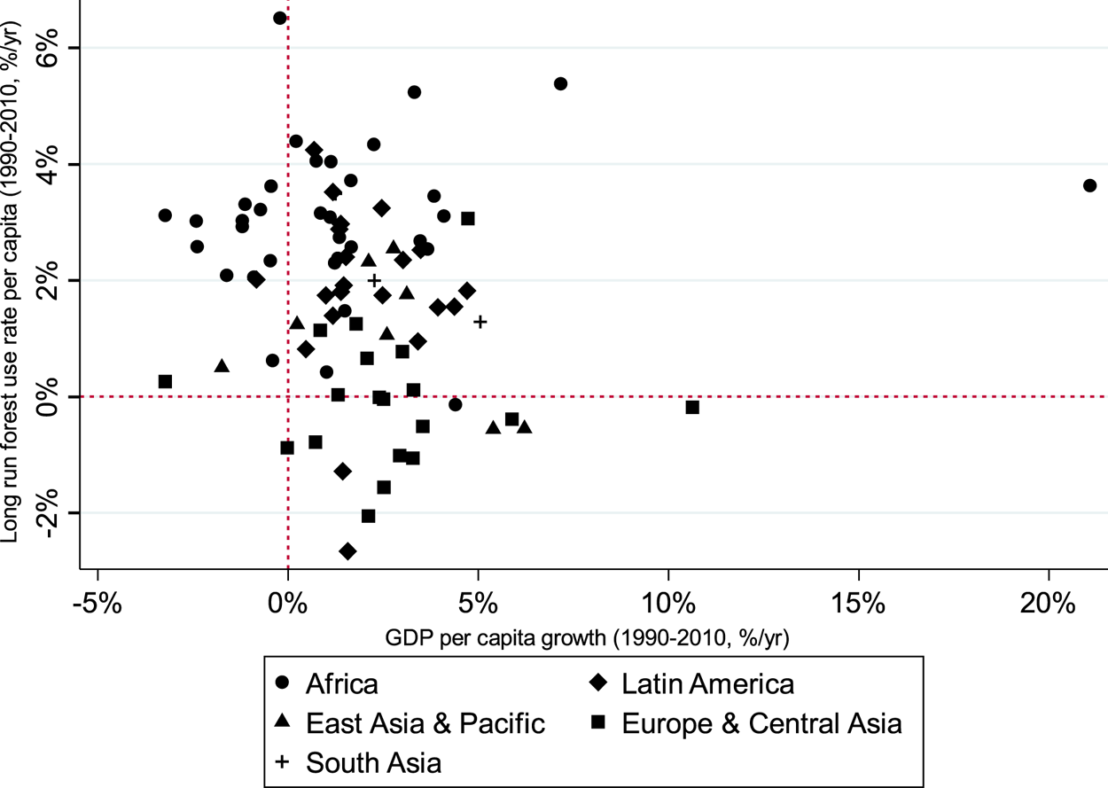
Figure 2. Growth rate of per capita income and loss of forest cover per capita.
In contrast, notice that there is a negative relationship between countries' initial level of forest cover per capita and their subsequent change in growth rate of forest cover per capita (see figure 3). This would imply that there is a beta convergence in all countries. In other words, countries with a high rate of forest cover change (strong deforestation) will tend to converge towards those with low rates of forest cover change (low deforestation).
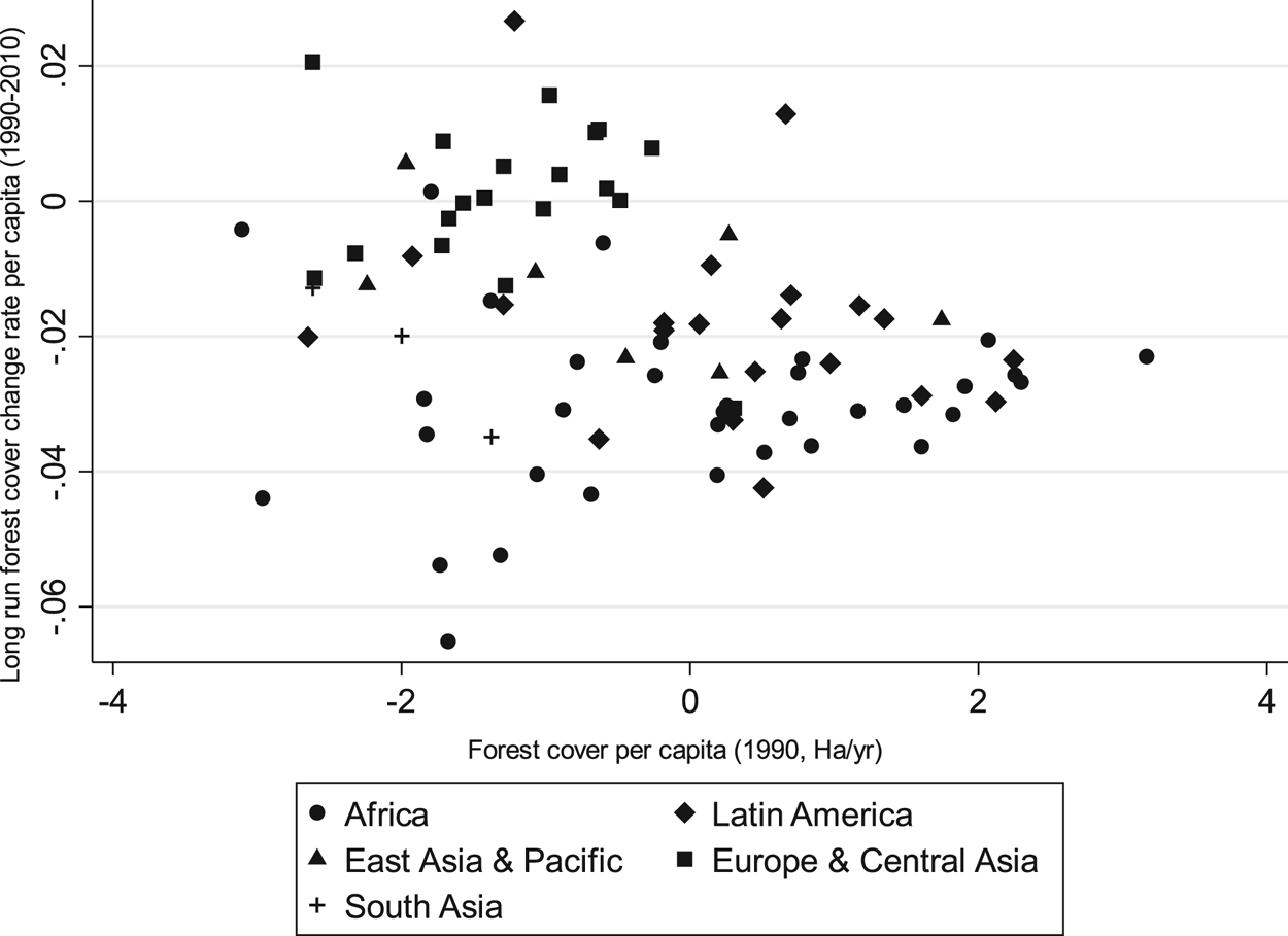
Figure 3. Convergence in deforestation (loss of forest cover).
Note: Forest cover per capita is in log.
5. Results
Tables 2 and 3 present the results of the estimation of the general long-run growth model and the restricted models respectively. Table 2 contains three columns: equations (1), (2) and (3). Equation (1) presents results for equation (1). Equation (2) presents the results for the same equation with the initial forest area per dollars instead of the initial level of forest cover per capita in order to capture forest use intensity. Finally, equation (3) presents the results of equation (1) including the log of income per capita averaged over time in each country instead of the average per capita income of the initial period to capture the impact of income level on the effect of time.
Table 2. General long-run growth model
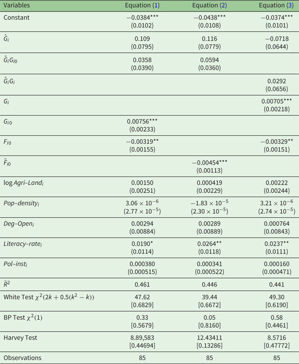
Notes: The dependent variable is the rate of change in percentage of forest area. Interpretation of the results in terms of deforestation rates should be followed by a negative sign. The standard deviations are in parentheses. Associated p-values are in brackets for each statistic. Levels of significance: * 10%, ** 5%, *** 1%. k is the number of non-constant variables.
Variables: ${\hat{F}_i}$ is long-run forest cover change rate per capita of country i; ${\hat{G}_i}$
 is long-run growth rate of GDP per capita of country i; Gi is the log of income per capita averaged over time in country i; Fi 0 and Gi 0 are the log of the per capita forest area and the log of per capita GDP of the early period of country i respectively; Agri–Landi is the agricultural land (% of land area) of country i; Deg–Openi is the degree of openness of country i; Pop–densityi is the population density of country i; Literacy–ratei and Pol–insti are the literacy rate and institutions of country i respectively.
Table 3. Restricted models

Notes: The dependent variable is the rate of change in percentage of forest area. Interpretation of the results in terms of deforestation rates should be followed by a negative sign. The standard deviations are in parentheses. Associated p-values are in brackets for each statistic. Levels of significance: ** 5%, *** 1%. k is the number of non-constant variables.
Variables: ${\hat{F}_i}$ is long-run forest cover change rate per capita of country i; ${\hat{G}_i}$
 is long-run growth rate of GDP per capita of country i; Gi is the log of income per capita averaged over time in country i; Fi 0 and Gi 0 are the log of the per capita forest area and the log of per capita GDP of the early period of country i respectively; Agri–Landi is the agricultural land (% of land area) of country i; Deg–Openi is the degree of openness of country i; Pop–densityi is the population density of country i; Literacy–ratei and Pol–insti are the literacy rate and institutions of country i respectively.
With regard to table 3, it also contains three columns. The first column presents the results of the Ordàs Criado et al. (Reference Ordas Criado, Valente and Stengos2011) model (equation (2)). The second column gives the results of the short-run Green Solow model. The third column presents the results of a basic EKC model (equation (3)) and the fourth column shows the results of the IPAT model (equation (4)).
Post-estimation tests focused on three tests of heteroscedasticity: the White test, the Breush-Pagan test and the Harvey test. Results show that only the Harvey heteroscedasticity hypothesis test is statistically significant at the 1 per cent level (see table 3). The global presence of heteroscedasticity justified the estimation of models using the White robust standard error method.
The results of table 2 show that the coefficient associated with the initial level area per capita is significantly negative at the 5 per cent level (see equations (1) and (2)). Similarly, the coefficient associated with the initial forest area per dollar is also negative and statistically significant at the 1 per cent level. This means that there is a strong and significant convergence across countries in terms of deforestation, that is, countries with a high rate of deforestation (or an important loss of forest cover) will converge to those with low deforestation rate (low degradation or increase in forest cover). In other words, countries converge in terms of policies that prevent deforestation. In contrast, the deforestation-income elasticity of 0.11 is statistically insignificant and different from unity. The coefficient of the interaction term between growth and the level of GDP per capita is not significantly different from zero. The coefficient of the interaction term between growth and the level of GDP per capita is not significantly different from zero. Both results show that the EKC hypothesis is not statistically significant.
The coefficients associated with the initial level and the average income of the countries are both significantly positive (equations (1) and (3)). This means that deforestation tends to decrease in high-income countries. However, the time effect (constant) is significantly negative. This shows that deforestation per capita tends to increase over time in each country regardless of its level of income, i.e., an increase of 3.84 per cent per year (see equation (1)). One plausible reason for this trend may be the large demographics in some regions, particularly in SSA. The literacy rate has a negative and significant effect on deforestation. This result means that the average improvement in the level of education (82 per cent) in tropical developing countries has raised public awareness about the need to preserve forest resources.
Table 3 shows that the restricted models can be rejected at the 1 per cent significance level only for the short-run Green Solow model (3), EKC model (4), and IPAT model (5). This means that the general specification is a better fit than these three restricted models. But it is weakly preferable to the model of Ordas Criado et al. (Reference Ordas Criado, Valente and Stengos2011), even if both models have the same explanatory power (adjusted R-squared is 0.46). The difference between these two specifications is focused on the interaction term between growth and the level of GDP per capita which is intended to test the EKC hypothesis. Since the interaction term is not significant in the long-term growth model, this may be the reason why the general specification is less preferred to the Ordas Criado et al. (Reference Ordas Criado, Valente and Stengos2011). One can therefore deduce that the growth and beta convergence effects are important in explaining forest cover changes since both effects are those predicted in the Ordas Criado et al. (Reference Ordas Criado, Valente and Stengos2011). In addition, these two models including convergence effects explain much more of the variation in the dependent variable than does the basic EKC model (4). As regards the short-term Green Solow model (3), its explanatory power is close to that of the basic EKC model (4). As for the EKC model, the interaction term is statistically significant (negative in the case of deforestation) at the 5 per cent level, which suggests the presence of a turning point at which economic growth has a beneficial effect on forest cover. The estimated income per capita turning point is at US$7,630.127 with a significance level of 5 per cent $(\textrm{s}.\textrm{d} = 0.5523)$ . This estimated income turning point is not out of the sample and corresponds to upper-middle-income countries, according to the 2010 World Bank Countries Classifications. The time effect for all the restricted models is negative and statistically significant at the 1 per cent level. This means that there is, on average, an increase in per capita forest cover use over time independently of economic growth. Finally, unsurprisingly, the IPAT model fits the data less well because it does not take into account the income interaction term and the convergence effect.
6. Discussion and conclusion
Previous empirical studies testing the relationship between deforestation and income are based on the traditional approach of analyzing the variables as levels. This paper provides an alternative understanding of this relationship by using the recent approach in terms of long-run growth rate. This approach allowed us to test multiple hypotheses about the drivers of environmental degradation in a single framework and avoid several of the econometric issues that have plagued the environmental Kuznets curve literature (Stern et al., Reference Stern, Gerlagh and Burke2017).
The main finding of this paper is that, just as with growth effects, beta convergence effects are also important in explaining changes in forest cover in tropical developing countries. The implication is that these countries converge in terms of policies that curb deforestation and forest degradation. Convergence policies could be a response to the growing awareness about the scarcity of forest resources in these countries and the importance of these resources in tackling the effects of climate change. They could also be due to initiatives taken at the international level under the REDD+ program, which aims to reduce emissions from deforestation and forest degradation in developing countries.
The convergence effects may be consistent with the forest transition theory (Mather, Reference Mather1992, Reference Mather2007) which describes a sequence over time where a forested region goes through a period of deforestation before the forest cover eventually stabilizes and starts to increase (Angelsen, Reference Angelsen2007). This transition has long been observed in developed countries. Nonetheless recent studies have shown that this phenomenon is also observed in developing countries (Kanninen et al., Reference Kanninen, Murdiyarso, Seymour, Angelsen, Wunder and German2007; Mather, Reference Mather2007; Xu et al., Reference Xu, Yang, Fox and Yang2007). Unlike the forest transition theory which does not explain how forest area changes, the convergence hypothesis might provide an explanation of forest transition based on the forces that govern the process of sustainable economic development. These forces include physical capital stock, population growth rates, and policies against climate change from deforestation and forest degradation through technological innovation and international initiatives such as REDD+.
Furthermore, findings show that the literacy rate has a strong positive effect on forest protection. This implies that deforestation and forest degradation tend to decline in tropical developing countries due to the improvement in education levels in these countries. Indeed, education plays an essential role in the protection of the environment because it makes the population aware of the need to preserve natural resources (Bimonte, Reference Bimonte2002).
The fact that the rate of deforestation is non-stationary (Polomé and Trotignon, Reference Polomé and Trotignon2016) has justified the long-term growth rate approach, which has helped to explain the long-term dynamics of forest area change in tropical developing countries. However, it is clear that this approach cannot address all the problems, including the unexplained short-term relationship and variation in countries' initial forest cover.
Supplementary material
The supplementary material for this article can be found at https://doi.org/10.1017/S1355770X2000039X.
Acknowledgements
I am very grateful to Professor David Stern and the anonymous reviewers for their helpful comments.


