


1 Introduction
A focused laser pulse with sufficient energy causes optical breakdown of a gas and produces a high-temperature, high-pressure volume of ionized gas (Meyerand & Haught Reference Meyerand and Haught1963). Even for a gas that is essentially transparent to the laser radiation, multi-photon ionization can produce free electrons that initiate a cascade process by which the gas becomes highly absorptive, leading to rapid heating (Morgan Reference Morgan1975; Harilal, Brumfield & Phillips Reference Harilal, Brumfield and Phillips2015). By the end of the laser pulse, typically 10 ns in duration for the applications considered, the plasma kernel appears 1–3 mm long and 0.2–1 mm wide. It also appears to be axisymmetric about the laser axis, but is often asymmetric in the direction of the laser (Adelgren et al. Reference Adelgren, Elliot, Knight, Zheltovodov and Beutner2001; Glumac & Elliott Reference Glumac and Elliott2007). The resulting expansion produces a shock wave that decouples from the kernel after approximately  $1~\unicode[STIX]{x03BC}\text{s}$, leaving behind a complex flow that mixes ambient gas with the hot kernel. In some cases, by approximately
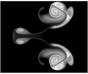
  $100~\unicode[STIX]{x03BC}\text{s}$, hot gas is ejected from the kernel along the laser axis, forming into an apparent vortex ring that can propagate beyond 10 mm from the breakdown location (figure 1a).

Figure 1. Laser-induced breakdown above a H2, 4.8 mm-diameter jet into atmospheric-pressure air (Retter, Glumac & Elliott Reference Retter, Glumac and Elliott2017). (a) The ejected hot gas (b) ignites the H2/air mixture approximately 10 mm from the breakdown location, indicated by the green dot, leading to (c) flame growth.
In a combustible mixture, the high temperature and presumably significant concentrations of radical species can ignite the gas and lead to a sustained flame. Such laser-seeded ignition is attractive because it deposits energy and radicals within a flow, away from material that might degrade, and with relatively precise control over timing and location (Ronney Reference Ronney1994; Phuoc Reference Phuoc2006). Ignition in various flow configurations has been studied (Lacaze et al. Reference Lacaze, Cuenot, Poinsot and Oschwald2009; Brieschenk, O’Byrne & Kleine Reference Brieschenk, O’Byrne and Kleine2013a; Massa & Freund Reference Massa and Freund2017; Gibbons et al. Reference Gibbons, Gehre, Brieschenk and Wheatley2018). Laser energy deposition has also been used in control for drag reduction (Riggins, Nelson & Johnson Reference Riggins, Nelson and Johnson1999) and controlling shock–shock interactions in supersonic flow (Kandala & Candler Reference Kandala and Candler2004; Adelgren et al. Reference Adelgren, Yan, Elliott, Knight, Beutner and Zheltovodov2005).
Ignition by laser-induced breakdown (LIB) can be affected by a number of hydrodynamic and chemical processes. The ejection in particular, appearing as the so-called third lobe in combustible mixtures, can both enhance the rate of flame growth by increasing its surface area, yet also inhibit ignition by high strain rates (Schmieder Reference Schmieder1981; Phuoc Reference Phuoc2006). Supporting this, Dumitrache et al. (Reference Dumitrache, VanOsdol, Limbach and Yalin2017) observed enhanced flame growth after suppressing the ejection with a pre-ionization pulse, which was thought to reduce flame stretching. Similarly, Torikai, Soga & Ito (Reference Torikai, Soga and Ito2017) showed that the ejection can extinguish a flame. In contrast, figure 1 shows that hot gas carried by the ejection can ignite gas some distance from the breakdown, which is potentially important in an inhomogeneous mixture with length scales comparable to the size of the ejection.
Even the qualitative character of the laser-induced ejection depends on local gas conditions. In multiple gases, Brieschenk, O’Byrne & Kleine (Reference Brieschenk, O’Byrne and Kleine2013b) observed ejection towards the laser source at pressure  $p=1~\text{atm}$ but away from the source at
  $p=30~\text{atm}$. In subsequent work, a similar reversal in ejection direction was observed for relatively mild changes in pressure (0.59 to 1 atm), as shown in figure 2 (J. E. Retter and G. S. Elliott, personal communication 2017). Although precise measurements of the energy deposition are difficult to obtain, these early-time luminosity images suggest that the reversal coincides with changes in the shape of kernel and that the underlying mechanism depends on the early-time energy distribution.

Figure 2. (a–d) Plasma luminosity in argon and air 10 ns after the laser pulse for a range of pressures. (e–h) Corresponding schlieren images 4.7 ms after the laser pulse showing ejection reversal (J. E. Retter and G. S. Elliott, personal communication). A 50 mJ, 532 nm single-mode laser with a focal length of 75 mm and pulse full-width-half-maximum of 7.7 ns was used. Emissions images were filtered with a central wavelength of 500 nm.
Other, similarly rapid and small energy depositions produce similar flows. For electrode discharges, a toroidal flow structure transports hot gas away from the breakdown region (Kono et al. Reference Kono, Niu, Tsukamoto and Ujiie1988; Thiele, Warnatz & Maas Reference Thiele, Warnatz and Maas2000; Bane, Ziegler & Shepherd Reference Bane, Ziegler and Shepherd2015). Kono et al. (Reference Kono, Niu, Tsukamoto and Ujiie1988) attributed this to low pressure in the spark gap caused by over-expansion of the plasma kernel, which induces an inward flow and production of vorticity that then propagates outward. In laser-induced breakdowns, low pressure produced by kernel over-expansion and an associated rarefaction wave were hypothesized to lead to a similar toroidal structure (Picone & Boris Reference Picone and Boris1983; Spiglanin et al. Reference Spiglanin, Mcilroy, Fournier, Cohen and Syage1995; Morsy & Chung Reference Morsy and Chung2002; Bradley et al. Reference Bradley, Sheppard, Suardjaja and Woolley2004). However, the specifics of how any low-pressure region leads to ejection or its reversal, especially its dependence on kernel shape (for example), remain unclear. Laser ablation of a solid surface produces a plume that ejects hot gas away from the target, which has also been attributed to over-expansion (Harilal et al. Reference Harilal, Miloshevsky, Diwakar, LaHaye and Hassanein2012). A different proposal is that the curved shock generated by the expanding plasma produces the vorticity (Svetsov et al. Reference Svetsov, Popova, Rybakov, Artemiev and Medveduk1997), which was subsequently developed into a model for ejections from laser-induced breakdowns (Massa & Freund Reference Massa and Freund2016). The relative contributions of the curved shock and overexpansion, however, have not been studied quantitatively. Furthermore, the connection between the early kernel geometry, vorticity generation and ultimate formation or reversal of the ejection remains unclear.
Although there are some apparent similarities with jetting by bubble collapse (e.g. Blake & Gibson Reference Blake and Gibson1987), the source of the driving pressure difference is fundamentally different. It has long been known that a collapsing bubble can become unstable (Plesset & Mitchell Reference Plesset and Mitchell1956), although it is unclear whether the gas-phase laser ejection, with its rapidly expanding hot plasma kernel and only weak subsequent contraction, can be described by similar mechanisms. We focus on mechanisms of vorticity generation. In the course of analysing the ensuing dynamics, we will draw qualitative analogies to the well-understood motion of uniform-density vortex rings (as in, for example, Picone & Boris (Reference Picone and Boris1988) and Ranjan et al. (Reference Ranjan, Niederhaus, Motl, Anderson, Oakley and Bonazza2007)). Although density variations persist locally, by the time this description becomes useful the flow speed is subsonic with weak compressibility effects. Incompressible vortex-ring theory is confirmed to predict the auto-advection speed of the ejected vorticity.
We focus on how the early kernel geometry leads to ejection and its reversal. The intense luminosity, rapid changes and small size of the plasma kernel make experimental diagnostics challenging, so we use well-resolved simulations of an idealized model breakdown (§ 2). While the breakdown physics is complex, a model geometry with basic front–rear asymmetry, coupled with an ideal-gas model, is confirmed to produce both ejection reversal and general agreement with vorticity measured with particle image velocimetry (PIV) (§ 3). To isolate vorticity production mechanisms, a corresponding semi-infinite geometry is introduced in § 4. These results are generalized to the finite-length geometry in § 5, where we analyse the effect of kernel asymmetry on vorticity generation. In § 6 it is shown how ejection and its reversal depend on the relative strength and position of ring-like vortical structures, which are ultimately determined by the kernel geometry.
2 Model configuration
2.1 Kernel model

Figure 3. The model breakdown kernel consists of two spherical caps joined by a conical section. The contact boundary thickness  $w\in [R_{2},R_{1}]$ varies with
  $s$, and the temperature
  $T\in [T_{\infty },T_{LIB}]$ varies with
  $n$.
$n$.
The model is based on early-time ( $t<100~\text{ns}$) imaging of plasma kernels. The specific geometric details of the resulting kernel can depend on the pulse energy (Harilal et al. Reference Harilal, Brumfield and Phillips2015), ambient pressure (Glumac & Elliott Reference Glumac and Elliott2007), gas composition (figure 2) as well as the mode of laser operation, which can lead to multiple points of apparent plasma initiation and alter the plasma boundary growth (Nishihara et al. Reference Nishihara, Freund, Glumac and Elliott2018). Simulations of the breakdown also show how the complex laser–plasma interaction can lead to the observed asymmetric structure (Kandala & Candler Reference Kandala and Candler2004; Alberti et al. Reference Alberti, Munafò, Koll, Nishihara, Pantano, Freund, Elliott and Panesi2019). In all these studies, the kernel is an approximately axisymmetric and elongated region with varying front–rear asymmetry. This consistent morphology motivates the model kernel introduced in figure 3: a high-temperature (
 $T_{LIB}$), high-pressure gas in a region constructed from two spherical caps joined by a conical section. The overall aspect ratio
  $\unicode[STIX]{x1D6FC}$ and ratio of cap radii
  $\unicode[STIX]{x1D6FD}$ are
 $$\begin{eqnarray}\unicode[STIX]{x1D6FC}\equiv \frac{L}{2R_{1}}\quad \text{and}\quad \unicode[STIX]{x1D6FD}\equiv \frac{R_{1}}{R_{2}}.\end{eqnarray}$$
 The breakdown is assumed to deposit zero momentum in the initially quiescent background ( $\boldsymbol{u}=\mathbf{0}$) and to occur isochorically (
 $\unicode[STIX]{x1D70C}=\unicode[STIX]{x1D70C}_{\infty }$), ensuring mass conservation. The kernel temperature blends smoothly with the ambient over local length scale
  $w$, which varies along the tangential coordinate
  $s$ as
 $$\begin{eqnarray}w(s)=\left\{\begin{array}{@{}ll@{}}R_{1},\quad & s<s_{1},\\ {\displaystyle \frac{s-s_{2}}{s_{1}-s_{2}}}R_{1}+{\displaystyle \frac{s-s_{1}}{s_{2}-s_{1}}}R_{2};\quad & s_{1}\leqslant s\leqslant s_{2},\\ R_{2},\quad & s_{2}<s,\end{array}\right.\end{eqnarray}$$
 where  $s_{1}$ and
  $s_{2}$ are set so the spherical sections are tangent to the conical section. The temperature
 $$\begin{eqnarray}T(n)=T_{\infty }+(T_{LIB}-T_{\infty })f(n)\end{eqnarray}$$
 varies with the normal coordinate  $n$, where
  $f(n)\equiv \frac{1}{2}[1-\tanh (\unicode[STIX]{x1D70E}n)]$ and
  $\unicode[STIX]{x1D70E}$ is set so
  $f(w/2)=0.1$ and
  $f(-w/2)=0.9$.
2.2 Governing equations
The flow equations are formulated for an ideal gas in axisymmetric cylindrical coordinates for the conserved flow variables  $\boldsymbol{Q}=\{\unicode[STIX]{x1D70C},\unicode[STIX]{x1D70C}u_{x},\unicode[STIX]{x1D70C}u_{r},\unicode[STIX]{x1D70C}e\}$, where
  $\unicode[STIX]{x1D70C}$ is the density, and
  $u_{x}$ and
  $u_{r}$ are the velocity components. The total energy
  $e$ and internal energy
  $e_{int}$ are
 $$\begin{eqnarray}e\equiv e_{int}+\frac{1}{2}|\boldsymbol{u}|^{2}\quad \text{and}\quad e_{int}=\frac{1}{\unicode[STIX]{x1D6FE}-1}\frac{p}{\unicode[STIX]{x1D70C}}=\frac{1}{\unicode[STIX]{x1D6FE}}c_{p}T,\end{eqnarray}$$
 where  $\unicode[STIX]{x1D6FE}=1.4$ is the ratio of specific heats and
  $c_{p}$ the specific heat at constant pressure. Unless otherwise noted,
  $T_{LIB}=26.9T_{\infty }$ and the Reynolds number
  $Re_{L}\equiv \unicode[STIX]{x1D70C}_{\infty }a_{\infty }L/\unicode[STIX]{x1D707}=4.4\times 10^{4}$ would correspond to a kernel length of
  $L=2~\text{mm}$ in air at
  $p_{\infty }=1~\text{atm}$ and
  $T_{\infty }=298~\text{K}$, where
  $\unicode[STIX]{x1D707}=1.8\times 10^{-5}~\text{Pa}~\text{s}$ is the dynamic viscosity and
  $a_{\infty }$ is the ambient speed of sound. For a strong ejection with speed
  $U=70~\text{m}~\text{s}^{-1}$ based on experimental imaging, a flow-velocity Reynolds number is
  $Re_{U}\equiv \unicode[STIX]{x1D70C}_{\infty }UL/\unicode[STIX]{x1D707}\approx 9200$. Although at early times
  $\unicode[STIX]{x1D6FE}=5/3$ would better represent the dissociated gas, a simulation with this
  $\unicode[STIX]{x1D6FE}$ evolves similarly, with net circulation differing by less than 6 % for the case considered in § 3.2. The bulk viscosity
  $\unicode[STIX]{x1D707}_{B}=0.6\unicode[STIX]{x1D707}$ is chosen as a model for air (Thompson Reference Thompson1971). The Prandtl number
  $Pr\equiv c_{p}\unicode[STIX]{x1D707}/\unicode[STIX]{x1D706}=0.72$ is also taken to be that of air, where
  $\unicode[STIX]{x1D706}$ is the thermal conductivity. The viscosity, specific heat, and thermal conductivity are assumed to be constant, which is clearly an approximation, especially in the hot plasma core. This perfect gas model is used to represent the range of possible phenomenologies and elucidate underlying hydrodynamic mechanisms rather than provide full quantitative detail at these extreme conditions. Previous work (Ghosh & Mahesh Reference Ghosh and Mahesh2008) suggests that additional physics such as chemistry or temperature-dependent transport properties would not significantly alter the flow pattern. Moreover, we show that the principal vorticity-generating mechanisms occur outside the hottest regions of the kernel. Our reduced model will be shown to reproduce key experimental observations in § 3.1, and viscous effects are assessed in more detail in § 4.5.
Of the six non-dimensional parameters  $\unicode[STIX]{x1D6FC}$,
  $\unicode[STIX]{x1D6FD}$,
  $T_{LIB}/T_{\infty }$,
  $Re_{L}$,
  $Pr$ and
  $\unicode[STIX]{x1D6FE}$, dependence on the geometry parameters
  $\unicode[STIX]{x1D6FC}$ and
  $\unicode[STIX]{x1D6FD}$ is our primary concern. Dependence on
  $Re_{R_{2}}\equiv \unicode[STIX]{x1D70C}_{\infty }a_{\infty }R_{2}/\unicode[STIX]{x1D707}$ will be considered in § 5.
A passive scalar  $\unicode[STIX]{x1D709}$ is used to track the evolving kernel, especially its boundary as labelled in figure 3. It is initialized with the signed distance
  $\unicode[STIX]{x1D709}(t=0)=n$ from the
  $n=0$ boundary and subsequently advects,
 $$\begin{eqnarray}\frac{\unicode[STIX]{x2202}(\unicode[STIX]{x1D70C}\unicode[STIX]{x1D709})}{\unicode[STIX]{x2202}t}+\unicode[STIX]{x1D735}\boldsymbol{\cdot }(\unicode[STIX]{x1D70C}\unicode[STIX]{x1D709}\boldsymbol{u})=0.\end{eqnarray}$$
The nominal contact boundary is thus
 $$\begin{eqnarray}\text{CB}\equiv \{(x,r)\mid \unicode[STIX]{x1D709}(x,r)=0\}.\end{eqnarray}$$
2.3 Simulation method
To discretize the governing equations, eighth-order, nine-point centred finite-difference stencils for first and second derivatives are used in concert with an explicit eighth-order, nine-point filter (Lele Reference Lele1992) applied at each time step. The shocks generated are relatively weak and modelled in the Navier–Stokes limit, with confirmed mesh independence. A shock-capturing scheme was not used due to concerns regarding the accuracy of vorticity generation by shock–shock or shock–vorticity interactions. Although standard schemes are designed and tested to produce accurate pressure and density fields (Bogey, De Cacqueray & Bailly Reference Bogey, De Cacqueray and Bailly2009; Lo, Blaisdell & Lyrintzis Reference Lo, Blaisdell and Lyrintzis2010), shear and vorticity generation is less often assessed. Studies with weighted essentially non-oscillatory schemes (WENO) suggest that it may not be suitable for the present analysis of vorticity production (Pirozzoli Reference Pirozzoli2002; Johnsen et al. Reference Johnsen, Larsson, Bhagatwala, Cabot, Moin, Olson, Rawat, Shankar, Sjögreen and Yee2010).
The governing equations at the  $r=0$ coordinate singularity are evaluated in the
 $r\rightarrow 0$ limit, with
 $$\begin{eqnarray}u_{r}=0,\quad \frac{\unicode[STIX]{x2202}\unicode[STIX]{x1D70C}}{\unicode[STIX]{x2202}r}=0,\quad \frac{\unicode[STIX]{x2202}p}{\unicode[STIX]{x2202}r}=0,\quad \frac{\unicode[STIX]{x2202}u_{x}}{\unicode[STIX]{x2202}r}=0\quad \text{and}\quad \frac{\unicode[STIX]{x2202}^{2}u_{r}}{\unicode[STIX]{x2202}r^{2}}=0\end{eqnarray}$$
 based on continuity and differentiability at  $r=0$ (e.g. Liu & Wang Reference Liu and Wang2009). The same interior stencils are also used at
  $r=0$, although they are constrained to enforce (2.4) using the fact that
  $\unicode[STIX]{x1D70C}$,
  $u_{x}$ and
  $e$ are even functions of
  $r$ and that
  $u_{r}$ is an odd function of
  $r$. Thus eighth-order spatial accuracy is achieved everywhere in the flow except the outer boundaries.
Table 1. Three simulations on successively coarser meshes are used to compute each LIB solution. For the stretched mesh, the mesh spacing corresponds to  $\unicode[STIX]{x0394}x_{min}=\unicode[STIX]{x0394}r_{min}$. The simulated times depend on the when the shock reaches the boundaries of meshes 1 and 2 and vary across cases.


Figure 4. Diagram showing the relative size of each mesh in table 1.
Because the kernel expands and gradients weaken in time, less spatial resolution is required at later stages. To reduce computational cost, the solution is computed using the three successively coarser meshes described in table 1 and figure 4. Before the shock reaches the mesh boundary, the solution is interpolated onto the next mesh with fourth-order bicubic polynomial splines. The first two meshes are uniform. The third mesh is stretched, with coordinates mapped independently from  $z_{1,2}\in [0,1]$ to
  $(x,r)$ using
 $$\begin{eqnarray}x=\frac{40L}{g}\left\{\frac{a}{2b}[\log (\cosh [b(z_{1}-1)])-\log (\cosh [bz_{1}])-\log (\cosh b)]+(1+a)z_{1}\right\}-20L,\end{eqnarray}$$
 $$\begin{eqnarray}\displaystyle r & = & \displaystyle \frac{40L}{g}\left\{\frac{a}{2b}\left[\log \left(\cosh \left[b\frac{z_{2}-1}{2}\right]\right)-\log \left(\cosh \left[b\frac{z_{2}+1}{2}\right]\right)-\log (\cosh b)\right]\right.\nonumber\\ \displaystyle & & \displaystyle +\left.(1+a)\frac{z_{2}+1}{2}\right\}-20L,\nonumber\end{eqnarray}$$
where
 $$\begin{eqnarray}g\equiv 1+a-\frac{a}{b}\log (\cosh b),\end{eqnarray}$$
 and  $a=112$ and
  $b=96.2$ are chosen so that mesh spacing in the region
  $x\in [-10L,10L]$,
  $r\in [0,10L]$ is effectively uniform, with
  $\unicode[STIX]{x0394}x$ and
  $\unicode[STIX]{x0394}r$ within 1 % of
  $\unicode[STIX]{x0394}x_{min}=\unicode[STIX]{x0394}r_{min}=0.003L$. All reported simulation results on this mesh are from this nearly uniform region. For most of the results the meshes in table 1 are used. Doubling the density of these meshes results in less than 1 % change in the net circulation and maximum flow velocity at
  $T_{LIB}=26.9T_{\infty }$. For the most intense cases in § 4.4, greater resolution (
 $1.25\times 10^{-4}L$) was required for this degree of mesh independence; for those conditions it was further verified that the post-shock pressure and velocity agree with the one-dimensional equivalent Riemann problem to within 0.4 %. To further assess accuracy, particularly for analysis of shock-generated vorticity, a still finer spacing is used (
 $2.5\times 10^{-5}L$), which confirmed insensitivity to the mesh.
At the outer boundary of the third mesh, the pressure  $p_{\infty }$ is imposed using the characteristic formulation of Thompson (Reference Thompson1990) in conjunction with the stabilization procedure of Poinsot & Lele (Reference Poinsot and Lele1992). In addition, a buffer zone (Freund Reference Freund1997; Colonius Reference Colonius2004), with a source term added to the flow equations
  $\boldsymbol{Q}_{t}+{\mathcal{N}}(\boldsymbol{Q})=\mathbf{0}$, is used with support near the boundary,
 $$\begin{eqnarray}\boldsymbol{Q}_{t}+{\mathcal{N}}(\boldsymbol{Q})=\max (\unicode[STIX]{x1D70E}_{x},\unicode[STIX]{x1D70E}_{r})(\boldsymbol{Q}_{\infty }-\boldsymbol{Q}),\end{eqnarray}$$
where
 $$\begin{eqnarray}\unicode[STIX]{x1D70E}_{x}=\left\{\begin{array}{@{}ll@{}}\left({\displaystyle \frac{|x|}{10L}}-1\right)^{2},\quad & x>10L\;\text{or}\;x<-10L\\ 0,\quad & \text{otherwise}\end{array}\right.\quad \unicode[STIX]{x1D70E}_{r}=\left\{\begin{array}{@{}ll@{}}\left({\displaystyle \frac{r}{10L}}-1\right)^{2},\quad & r>10L\\ 0,\quad & \text{otherwise}\end{array}\right.\end{eqnarray}$$
 and  $\boldsymbol{Q}_{\infty }\equiv \{\unicode[STIX]{x1D70C}_{\infty },0,0,\unicode[STIX]{x1D70C}_{\infty }e_{\infty }\}$. All simulations are advanced with an explicit fourth-order Runge–Kutta scheme using a time step
 $$\begin{eqnarray}\unicode[STIX]{x0394}t=\min _{\{mesh\}}\frac{\text{CFL}}{{\displaystyle \frac{|u_{x}|+a}{\unicode[STIX]{x0394}x}}+{\displaystyle \frac{|u_{r}|+a}{\unicode[STIX]{x0394}r}}},\end{eqnarray}$$
 where  $a$ is the local speed of sound and
  $\text{CFL}=0.8$.

Figure 5. The model kernel is fit to the 50 % normalized luminosity level of the early-time kernel image, reproduced here from figure 2(b).  $R_{1}$ and
  $R_{2}$ are chosen as the maximum radial extents of the left and right halves, respectively, with their centres chosen such that the model kernel matches in length.
3 Ejection phenomenology
3.1 Comparison with experiment
We first confirm that the model reproduces key experimental observations. For this, the model parameters  $\unicode[STIX]{x1D6FC}$,
  $\unicode[STIX]{x1D6FD}$, and
  $L$ are based on early-time imaging – figure 5 shows the fitting process – and
  $T_{LIB}$ is chosen such that the energy deposited matches measurement. Given the assumptions (idealized geometry, uniform and instantaneous energy deposition, ideal-gas properties), we have no expectation of precise agreement. Still, figure 6 shows that the vorticity agrees qualitatively with measurement: the predominantly
  $\unicode[STIX]{x1D714}_{\unicode[STIX]{x1D703}}<0$ vorticity is ejected leftward, whereas the predominantly
  $\unicode[STIX]{x1D714}_{\unicode[STIX]{x1D703}}>0$ vorticity is located farther from the axis and, in this case, moves slowly rightward. There is quantitative agreement in net circulation until at least
  $200~\unicode[STIX]{x03BC}\text{s}$, consistent with the similar auto-advection speeds of the ejection. By
  $500~\unicode[STIX]{x03BC}\text{s}$ the on-average axisymmetry is apparently disrupted by shot-to-shot variation. Onset of three-dimensional instabilities will affect this late-time development, though the degree of comparison here suggests that it does not alter the mechanisms of vorticity production leading to the organized motion, which will be shown to occur well before the times of figure 6. The relative temperature distribution in figure 7 shows similar agreement with different measurements (Glumac, Elliott & Boguszko Reference Glumac, Elliott and Boguszko2005): the ambient gas breaches the kernel at approximately
  $50~\unicode[STIX]{x03BC}\text{s}$, and the hottest gas is pushed outward from the symmetry axis.

Figure 6. (a) PIV-measured azimuthal vorticity averaged over 100 breakdowns in 1 atm air (Koll, Elliott & Freund Reference Koll, Elliott and Freund2020), with the same laser configuration as in figure 2. (b) Simulation with the present model using  $\unicode[STIX]{x1D6FC}=3.23$,
  $\unicode[STIX]{x1D6FD}=1.24$ and
  $L=1.84~\text{mm}$ based on figure 5. Although simulation of an individual breakdown leads to sharper features than the averaged experimental data (note the different colour levels), the net circulation
  $\unicode[STIX]{x1D6E4}\equiv \iint \unicode[STIX]{x1D714}_{\unicode[STIX]{x1D703}}\,\text{d}x\,\text{d}r$ in the
  $r>0$ half-plane matches to within 10 % at
  $200~\unicode[STIX]{x03BC}\text{s}$, with
  $\unicode[STIX]{x1D6E4}_{\{r>0\}}$ and
  $\unicode[STIX]{x1D6E4}_{\{r<0\}}$ differing by less than 1 % in the experiment.

Figure 7. (a–c) Temperature averaged over 200 breakdowns in 0.97 atm air (Glumac et al. Reference Glumac, Elliott and Boguszko2005), adapted here with permission. (d–f) Simulation with the present model using  $\unicode[STIX]{x1D6FC}=3.24$,
  $\unicode[STIX]{x1D6FD}=1.92$ and
  $L=2.71~\text{mm}$ based on plasma kernel imaging at 25 ns in the corresponding experiments. A direct comparison of temperature values is not informative for the perfect gas model of the present simulations.
3.2 Kernel evolution and ejection

Figure 8. Relative mean pressure and temperature (3.1) and kernel volume, with  $V_{0}$ the initial volume. Fainter lines show only mild variation due to geometry (
 $\unicode[STIX]{x1D6FC}\in [2,4]$,
  $\unicode[STIX]{x1D6FD}\in [1.2,3.0]$) relative to the
  $\unicode[STIX]{x1D6FC}=3$,
  $\unicode[STIX]{x1D6FD}=3$ baseline case;
  $\unicode[STIX]{x1D6FC}=4$ kernels attain
  $\min \overline{p}$ and
  $\max V_{\unicode[STIX]{x1D6FA}}$ later in time.
A case with  $\unicode[STIX]{x1D6FC}=3$ and
  $\unicode[STIX]{x1D6FD}=3$ is described here in detail. The geometric parameters are based on general observations of luminous regions in experiments, and a full range is considered subsequently. Figure 8 shows the kernel volume, based on the nominal contact boundary (2.3), and its mean interior pressure and temperature, defined as
 $$\begin{eqnarray}\overline{p}\equiv \frac{\unicode[STIX]{x1D6FE}-1}{\unicode[STIX]{x1D6FE}}c_{p}\overline{\unicode[STIX]{x1D70C}}\overline{T}\quad \text{and}\quad \overline{T}\equiv \frac{\unicode[STIX]{x1D6FE}}{c_{p}}\overline{e}_{int},\end{eqnarray}$$
where
 $$\begin{eqnarray}\overline{\unicode[STIX]{x1D70C}}\equiv \frac{1}{V_{\unicode[STIX]{x1D6FA}}}\int _{\unicode[STIX]{x1D6FA}}\unicode[STIX]{x1D70C}\,\text{d}V\quad \text{and}\quad \overline{e}_{int}\equiv \frac{1}{\overline{\unicode[STIX]{x1D70C}}V_{\unicode[STIX]{x1D6FA}}}\int _{\unicode[STIX]{x1D6FA}}\unicode[STIX]{x1D70C}e_{int}\,\text{d}V,\end{eqnarray}$$
 with  $\unicode[STIX]{x1D6FA}$ the region enclosed by the contact boundary (2.3) and
  $V_{\unicode[STIX]{x1D6FA}}$ its volume. Both
  $\overline{T}$ and
  $\overline{p}$ decrease rapidly as the kernel expands, producing the shock wave visualized in figure 9(a). The part of this shock emanating from the conical section of the model geometry, approximately normal to the axis, is strongest, which is consistent with experimental observations (Gregorčič, Diaci & Možina Reference Gregorčič, Diaci and Možina2013). The kernel reaches its maximum volume at
  $t\approx 0.5L/a_{\infty }$, at which point the interior pressure has dropped below
  $p_{\infty }$ and subsequently begins to equilibrate.
This early dynamics induces the complex flow shown in figure 9(b), which marks the beginning of the ejection. A region of negative- $x$ momentum near
  $r=0$ on the right side of the kernel is associated with negative vorticity, which can be interpreted as auto-advecting leftward. Most of this momentum is in the dense inward-flowing ambient gas outside the kernel boundary. It breaches the hot, low-density (
 $\unicode[STIX]{x1D70C}\approx \unicode[STIX]{x1D70C}_{\infty }/8$) kernel at
  $t\approx 9.0L/a_{\infty }$, as shown in figure 9(c).

Figure 9. Formation of a leftward ejection with  $\unicode[STIX]{x1D6FC}=3$ and
  $\unicode[STIX]{x1D6FD}=3$. (a) The shock, visualized with the pressure, propagates outwards from the contact boundary (CB); the initial kernel is shown in grey. (b–d) The vorticity distribution,
  $\unicode[STIX]{x1D70C}\boldsymbol{u}$ vectors, and ejection as labelled. The dotted box in (b) highlights the region of negative
  $x$-momentum leading to the ejection. Momentum instead of velocity vectors are shown due to the density variation.

Figure 10. Circulation and maximum speed. The dashed line at  $\unicode[STIX]{x1D6E4}=-0.14La_{\infty }$ is shown for reference. Before
  $t=1.39L/a_{\infty }$,
  $\max |\boldsymbol{u}|$ is associated with the shock and marked by a dotted line.
Figure 10 shows the circulation
 $$\begin{eqnarray}\unicode[STIX]{x1D6E4}\equiv \iint \unicode[STIX]{x1D714}\,\text{d}r\,\text{d}x,\end{eqnarray}$$
where
 $$\begin{eqnarray}\unicode[STIX]{x1D714}\equiv \unicode[STIX]{x1D714}_{\unicode[STIX]{x1D703}}=\frac{\unicode[STIX]{x2202}u_{r}}{\unicode[STIX]{x2202}x}-\frac{\unicode[STIX]{x2202}u_{x}}{\unicode[STIX]{x2202}r}.\end{eqnarray}$$
 Rapid production of circulation occurs before  $t=2L/a_{\infty }$, which coincides with the changes in pressure seen in figure 8. Beyond this time the flow is subsonic and qualitatively consistent with auto-advection of existing vorticity, albeit in a variable-density fluid. This is not expected to be significant in interpreting the evolution since 79 % of the volume within
  $L$ of the kernel centre has
  $\unicode[STIX]{x1D70C}>0.8\unicode[STIX]{x1D70C}_{\infty }$. After the kernel is breached at
  $t\approx 9L/a_{\infty }$ (figure 9c), the circulation remains approximately constant, and the negative vorticity separates from the nominal breakdown location and propagates as a hot vortex ring (figure 9d). By
  $t=60L/a_{\infty }$ its speed is within 20 % of the standard auto-advection speed
  $U$ of an incompressible and constant-density vortex ring,
 $$\begin{eqnarray}U=\frac{\unicode[STIX]{x1D6E4}_{0}}{4\unicode[STIX]{x03C0}r_{0}}\left[\ln \left(\frac{8r_{0}}{a}\right)-\frac{1}{4}\right].\end{eqnarray}$$
 For making this estimate, its nominal position  $(x_{0},r_{0})$ is marked by the peak vorticity
  $\unicode[STIX]{x1D714}_{0}$, the circulation
  $\unicode[STIX]{x1D6E4}_{0}$ is the total within
  $x\in [x_{0}-2r_{0},x_{0}+2r_{0}]$ (as in Archer, Thomas & Coleman (Reference Archer, Thomas and Coleman2008)), and the radius
  $a=\sqrt{\unicode[STIX]{x1D6E4}_{0}/\unicode[STIX]{x03C0}\unicode[STIX]{x1D714}_{0}}$ is such that a uniform vortex core with
  $\unicode[STIX]{x1D714}=\unicode[STIX]{x1D714}_{0}$ would have the same circulation. The specific sources of vorticity will be analysed in detail in §§ 4 and 5.
3.3 Dependence on kernel geometry
The hydrodynamic development depends on the initial kernel geometry, which we vary over  $\unicode[STIX]{x1D6FC}\in [2,12]$ and
  $\unicode[STIX]{x1D6FD}\in [1/3,3]$ to include a range of observations (Glumac & Elliott Reference Glumac and Elliott2007; J. E. Retter and G. S. Elliott, personal communication 2017). Figure 11 shows that the net circulation
  $\unicode[STIX]{x1D6E4}$ changes sign with both
  $\unicode[STIX]{x1D6FC}$ and
  $\unicode[STIX]{x1D6FD}$, with corresponding reversals in the ejection, quantified by its length
  $L_{E}$. Fore–aft symmetry effects (
 $\unicode[STIX]{x1D6FD}\lessgtr 1$), which appear to correspond to early-time luminosity imaging (figure 2b–d), can obviously lead to reversal, with more asymmetric kernels (larger
  $\unicode[STIX]{x1D6FD}$ or
  $1/\unicode[STIX]{x1D6FD}$) producing greater circulation and a more pronounced ejection. Closer inspection also suggests that the ejected vortex ring of such kernels has a smaller radius and propagates faster (e.g.
  $\unicode[STIX]{x1D6FD}=1.5$ versus
  $\unicode[STIX]{x1D6FD}=3$), consistent with (3.3). For near-symmetric kernels (
 $1/1.2\lesssim \unicode[STIX]{x1D6FD}\lesssim 1.2$) a distinct ejection is not observed, and the vorticity instead collects into a ring pair that travels outward from the symmetry axis. More curiously, increasing the aspect ratio beyond
  $\unicode[STIX]{x1D6FC}\approx 5$ also leads to reversal, though the rightward ejection is somewhat weaker than its leftward counterpart. Details of the ejection failure at
  $\unicode[STIX]{x1D6FD}\approx 1.2$ and the reversal at
  $\unicode[STIX]{x1D6FC}\approx 5$ will be discussed in § 6.

Figure 11. Dependence of the ejection character on  $\unicode[STIX]{x1D6FC}$ and
  $\unicode[STIX]{x1D6FD}$, visualized with the vorticity and temperature at
  $t=100L/a_{\infty }$, with the initial kernel in grey. Each data point is coloured by the net circulation
  $\unicode[STIX]{x1D6E4}$ (3.2), and arrows correspond to the ejection length
  $L_{E}$, taken to be the axial distance from the centre of the initial kernel to the point of peak vorticity
  $\max |\unicode[STIX]{x1D714}|$. Only
  $L_{E}>L$ arrows are shown to indicate cases in which a clear ejection is observed.
4 Mechanisms of vorticity generation: a semi-infinite analogue
4.1 Configuration
An analogous, semi-infinite geometry (figure 12) is introduced here to isolate vorticity-generating mechanisms from subsequent vortex formation and interaction dynamics, which are considered in more detail subsequently. The thermal initial condition (2.1) is used for a cylindrical section that extends effectively to  $x\rightarrow -\infty$ and capped by a hemisphere at
  $x=0$. Practically, this configuration was implemented in a sufficiently long domain to preclude interactions between the ends for the times considered. Without a length scale analogous to
  $L$, we use
  $Re_{R_{2}}\equiv \unicode[STIX]{x1D70C}_{\infty }a_{\infty }R_{2}/\unicode[STIX]{x1D707}=2400$ to be consistent with the baseline
  $\unicode[STIX]{x1D6FC}=3$,
  $\unicode[STIX]{x1D6FD}=3$ geometry for which
  $L=18R_{2}$. This configuration has four non-dimensional parameters (
 $Re_{R_{2}}$,
  $T_{LIB}/T_{\infty }$,
  $\unicode[STIX]{x1D6FE}$,
  $Pr$), which is simplifying since it avoids the
  $\unicode[STIX]{x1D6FC}$ and
  $\unicode[STIX]{x1D6FD}$ parameters of § 3.3. Dependence on
  $Re_{R_{2}}$ is quantified in § 4.5.

Figure 12. The semi-infinite geometry consists of an infinitely long cylindrical section and a hemispherical cap.
The flow generated by this configuration is shown in figure 13. As for the finite- $L$ cases, the expanding kernel produces a shock, behind which there is transient subambient pressure near the kernel (figure 13a). By
  $t=40R_{2}/a_{\infty }$ (figure 13b), obvious negative vorticity has been produced near the end, and by
  $t=236R_{2}/a_{\infty }$ the associated negative-
 $x$ flow at the end of the kernel has penetrated into the low-density kernel (figure 13c). The evolution after this point is phenomenologically consistent with auto-advection of the vorticity, with a maximum velocity less than
  $0.1a_{\infty }$. The faster vorticity advection near the axis resembles that of the finite-length cases (figure 9c).

Figure 13. (a) The shock decouples from the kernel, initially in the grey region, and (b) leaves behind a region of negative vorticity that (c) penetrates into the hot, low-density kernel. Vectors correspond to  $\unicode[STIX]{x1D70C}\boldsymbol{u}$.
4.2 Vorticity generation by the shock
By  $t=1.19R_{2}/a_{\infty }$, the kernel has cooled from
  $26.9T_{\infty }$ initially to a peak of
  $13.0T_{\infty }$, and the shock has decoupled from the hot gas, as shown in figure 14(a), leaving a triangle-like region of negative vorticity behind it. Positive vorticity is also produced along the contact boundary during this early expansion, though this is largely cancelled by a subsequent mechanism, which will be discussed in § 4.3.

Figure 14. (a) Negative vorticity generation by the shock at  $t=1.19R_{2}/a_{\infty }$ is (b) partially cancelled by positive baroclinic torque. The initial kernel is shaded grey in (a).
The dominant source of the negative vorticity is tangential variation in the shock strength, quantified by the pressure immediately behind the shock (figure 15). Away from the cylindrical–spherical junction, it matches the pressure at these short times for corresponding spherical and cylindrical cases. It is the faster decay of the spherical shock that leads to the pressure gradient between the two regions.
Theoretical estimates for shock-generated vorticity were independently derived by Truesdell (Reference Truesdell1952) and Lighthill (Reference Lighthill1957) and generalized by Hayes (Reference Hayes1957). For an unsteady, axisymmetric shock of varying strength,
 $$\begin{eqnarray}\unicode[STIX]{x1D714}=\frac{\unicode[STIX]{x1D70C}_{s}}{\unicode[STIX]{x1D70C}_{\infty }}\left(1-\frac{\unicode[STIX]{x1D70C}_{\infty }}{\unicode[STIX]{x1D70C}_{s}}\right)^{2}\frac{\unicode[STIX]{x2202}U}{\unicode[STIX]{x2202}s},\end{eqnarray}$$
 where  $\unicode[STIX]{x1D70C}_{s}$ is the density behind the shock,
  $U$ is the shock speed and
  $s$ is the local tangent coordinate. Applying shock-jump relations yields
 $$\begin{eqnarray}\unicode[STIX]{x1D714}=\frac{\unicode[STIX]{x1D6FE}+1}{4\unicode[STIX]{x1D6FE}}\frac{\unicode[STIX]{x1D70C}_{s}}{\unicode[STIX]{x1D70C}_{\infty }}\left(1-\frac{\unicode[STIX]{x1D70C}_{\infty }}{\unicode[STIX]{x1D70C}_{s}}\right)^{2}\frac{1}{\sqrt{{\displaystyle \frac{\unicode[STIX]{x1D6FE}-1}{2\unicode[STIX]{x1D6FE}}}+{\displaystyle \frac{\unicode[STIX]{x1D6FE}+1}{2\unicode[STIX]{x1D6FE}}}{\displaystyle \frac{p_{s}}{p_{\infty }}}}}{\displaystyle \frac{a_{\infty }}{p_{\infty }}}\frac{\text{d}p_{s}}{\text{d}s},\end{eqnarray}$$
 where  $p_{s}$ is the pressure behind the shock. Thus, the region of negative vorticity in figure 14 is produced by the tangential pressure gradient in figure 15(a) and grows in size as this region grows along the shock front.

Figure 15. Pressure behind the shock for the (a) axisymmetric semi-infinite kernel and (b) corresponding spherically and cylindrically symmetric cases. 1-D, one-dimensional; Cyl., cylindrical; Sph., spherical.
In figure 14(b), it is also evident that a distributed baroclinic torque behind the shock acts to cancel the shock-generated vorticity. The misalignment of  $\unicode[STIX]{x1D735}\unicode[STIX]{x1D70C}$ and
  $\unicode[STIX]{x1D735}p$ that drives this is illustrated schematically in figure 16(a). In the effectively spherical and cylindrical regions, pressure and density closely match the corresponding one-dimensional case and therefore have parallel gradients. Between these regions, the higher pressure behind the cylindrical shock (figure 16b) leads to misalignment.

Figure 16. (a) Schematic showing the post-shock misalignment of  $\unicode[STIX]{x1D735}\unicode[STIX]{x1D70C}$ and
  $\unicode[STIX]{x1D735}p$ between the effectively one-dimensional regions, and (b) corresponding pressure profiles, where
  $r_{s}$ is the position of the shock.


Figure 18. Evolution of the mean kernel pressure (3.1) and pressure field, with slices at  $r/R_{2}=0$, 2, 4 and 6 showing the
  $x$-component of its gradient. Here,
  $\overline{p}$ is computed by integration over
  $x\geqslant -9R_{2}$ only, which corresponds to right half of the
  $\unicode[STIX]{x1D6FC}=3$,
  $\unicode[STIX]{x1D6FD}=3$ kernel in which
  $L=18R_{2}$.
The net effect of these two vorticity sources – negative at the shock and positive behind the shock – is quantified by the negative circulation  $\unicode[STIX]{x1D6E4}_{-}$,
 $$\begin{eqnarray}\unicode[STIX]{x1D6E4}_{-}(t)\equiv \iint _{\unicode[STIX]{x1D714}<0}\unicode[STIX]{x1D714}(t)\,\text{d}x\,\text{d}r,\end{eqnarray}$$
shown in figure 17, which decreases monotonically as the shock propagates. Their respective contributions can be estimated by integrating (4.1) for the shock-generated circulation,
 $$\begin{eqnarray}\unicode[STIX]{x1D6E4}_{s}(t)\equiv \iint \unicode[STIX]{x1D714}(t)\,\text{d}n\,\text{d}s,\end{eqnarray}$$
 using the shock speed for  $\text{d}n=U\,\text{d}t$, which upon applying the shock-jump relation as in (4.1) yields
 $$\begin{eqnarray}\unicode[STIX]{x1D6E4}_{s}(t)=\frac{\unicode[STIX]{x1D6FE}+1}{4\unicode[STIX]{x1D6FE}}\int _{\unicode[STIX]{x1D70F}=t_{b}}^{t}\int _{-\infty }^{0}\frac{\unicode[STIX]{x1D70C}_{s}}{\unicode[STIX]{x1D70C}_{\infty }}\left(1-\frac{\unicode[STIX]{x1D70C}_{\infty }}{\unicode[STIX]{x1D70C}_{s}}\right)^{2}\frac{a_{\infty }^{2}}{p_{\infty }}\frac{\text{d}p_{s}}{\text{d}s}\,\text{d}s\,\text{d}\unicode[STIX]{x1D70F}.\end{eqnarray}$$
 Because  $p_{s}=p_{s}(s)$, the
  $s$-integration can be recast as
 $$\begin{eqnarray}\unicode[STIX]{x1D6E4}_{s}(t)=\frac{\unicode[STIX]{x1D6FE}+1}{4\unicode[STIX]{x1D6FE}}\int _{t_{b}}^{t}\int _{p_{cyl}(\unicode[STIX]{x1D70F})}^{p_{sph}(\unicode[STIX]{x1D70F})}\frac{\unicode[STIX]{x1D70C}_{s}}{\unicode[STIX]{x1D70C}_{\infty }}\left(1-\frac{\unicode[STIX]{x1D70C}_{\infty }}{\unicode[STIX]{x1D70C}_{s}}\right)^{2}\frac{a_{\infty }^{2}}{p_{\infty }}\,\text{d}p_{s}\,\text{d}\unicode[STIX]{x1D70F},\end{eqnarray}$$
 where  $p_{cyl}$ and
  $p_{sph}$ are the corresponding cylindrical and spherical shock pressures. The shock formation time
  $t_{b}$ is the time at which the compression wave steepens into a shock, as marked by
  $\unicode[STIX]{x1D70C}$ reaching its maximum value, which always occurs on the shock in these simulations. The value of
  $t_{b}$ is calculated from the spherical configuration; the cylindrical shock forms only approximately 10 % earlier (figure 15b). Conclusions do not depend on this choice since the pre-shock generation of vorticity is small, as seen in the figure 17 inset.
By time  $t=t_{sw}$, with
  $\dot{\unicode[STIX]{x1D6E4}}_{s}t_{sw}<0.1\unicode[STIX]{x1D6E4}_{s}$ signifying the nominal end of significant shock-driven vorticity generation, the shock is too weak to produce even 10 % additional circulation. By this time it is approximately
  $10R_{2}$ from the kernel, so it is also unclear that any small addition would couple with the ejection dynamics. The negative circulation remaining after the post-shock cancellation, which removes 72 % of
  $\unicode[STIX]{x1D6E4}_{s}$ by
  $t_{sw}$ (figure 17), will be shown to constitute a relatively small portion of the peak negative circulation, attained as the ambient gas begins to penetrate into the kernel (§ 4.3).
Vorticity generation by the differential blast strength has been connected to vorticity production in other configurations as well (Svetsov et al. Reference Svetsov, Popova, Rybakov, Artemiev and Medveduk1997; Bane et al. Reference Bane, Ziegler and Shepherd2015); for the present case, analysis indicates that a large portion is cancelled by the post-shock rarefaction. We also note that while this idealized spherical–cylindrical geometry facilitates analysis, shock generation of vorticity does not depend on it specifically, only on the increasing shock strength away from the end of the kernel. This key behaviour is supported by experiments, in which measured shock speeds are faster in  $r$ than in
  $x$ (Gregorčič et al. Reference Gregorčič, Diaci and Možina2013), consistent with the observation that the shock evolves from elongated to spherical (Harilal et al. Reference Harilal, Brumfield and Phillips2015; Limbach Reference Limbach2015).
4.3 Baroclinic generation at the kernel boundary
The second mechanism we consider operates over a longer time than the shock, until  $t\approx 87R_{2}/a_{\infty }=15t_{sw}$. A low-pressure region around the hot kernel remnant leads to
  $\unicode[STIX]{x1D735}p$ that is approximately perpendicular to the strong
  $\unicode[STIX]{x1D735}\unicode[STIX]{x1D70C}$ associated with the kernel boundary (figure 18). Pressure traces show the important
  $x$-component of this gradient and the trailing rarefaction behind the shock. The corresponding evolution of
  $\unicode[STIX]{x1D6E4}_{-}$ in figure 19 indicates that this baroclinic torque produces more vorticity than the net left behind the shock. Approximately 28 % of the peak negative circulation
  $\unicode[STIX]{x1D6E4}_{max}^{-}$, attained at
  $t=87R_{2}/a_{\infty }$, is produced by the shock before
  $t_{sw}$. However, unlike the shock, which deposits vorticity in the dense ambient gas, this mechanism produces vorticity in hot gas with
  $\unicode[STIX]{x1D70C}\lesssim \unicode[STIX]{x1D70C}_{\infty }/5$, so its long-term contribution to the flow is anticipated to be somewhat suppressed. The vorticity from the shock, though deposited at early times, persists and appears unaffected by the baroclinic generation near the contact boundary.

Figure 19. Vorticity production near the contact boundary. The short time window of figure 17 covering the period of significant generation by the shock is indicated for reference. The peak negative circulation  $\unicode[STIX]{x1D6E4}_{max}^{-}$ is attained at
  $t=87R_{2}/a_{\infty }$.
The low-pressure region in figure 18 is due to the expansion following the shock. Figure 20(a) depicts Cartesian, cylindrical and spherical analogues, which all produce a shock with a trailing rarefaction shown in figure 20(b). In the cylindrical and spherical geometries, this region, including the kernel itself (figure 20c), has  $p<p_{\infty }$ before equilibrating, which corresponds to the low pressure in figure 18.

Figure 20. (a) Analogous one-dimensional configurations produce (b) a trailing rarefaction behind the shock and low-pressure region around the kernel, whose (c) mean pressure can become sub-ambient. Profiles in (b) are shown at  $t=6.3R_{2}/a_{\infty }$, with triangle symbols marking the location of the contact boundary.
The mechanism by which expansion waves lead to this low pressure is illustrated for the simpler one-dimensional case in figure 21. Figure 21(a) shows the pressure and characteristic velocities at  $x=0$. For clarity a sharpened-boundary case
  $w=R_{2}/100$ is also shown to better highlight the distinct expansions that progressively decrease the pressure. Each expansion phase corresponds to a rarefaction reaching
  $x=0$ (figure 21b), with the first originating at the kernel boundary and subsequent rarefactions produced by reflection. Between expansions, the state of the gas at
  $x=0$ is constant. Figure 21(a) also shows that a kernel with a diffuse boundary, matching our simulations with
  $w=R_{2}$, tracks this behaviour though with the overlapping rarefactions smoothing the profiles. Viscous effects are sufficiently weak that increasing
  $Re_{R_{2}}$ by a factor of 2 results in less than 1 % change in
  $p$ and
  $u\pm a$ in figure 21(a).

Figure 21. (a) Evolution of pressure and characteristic velocities at  $x=0$ for the Cartesian configuration, showing a series of expansions that cause the pressure to decrease, both for a sharp boundary (——)
  $w=R_{2}/100$ and for the simulated CB scale (– – –)
  $w=R_{2}$. (b) Pressure evolution in
  $x$–
$x$– $t$ (
$t$ ( $w=R_{2}/100$) and subset of characteristics.
The same mechanism produces low pressure near the origin in the radial configurations. However, a rarefaction wave propagating towards  $r=0$ must expand outward-travelling gas into a larger volume than a corresponding wave in a Cartesian geometry (Friedman Reference Friedman1961), resulting in
  $p<p_{\infty }$ as noted in figure 20(b).
Though direct correspondence to the one-dimensional cases diminishes rapidly in time, a nearly one-dimensional character holds during the expansion in approximately cylindrical and spherical regions, where there is only weak misalignment of  $\unicode[STIX]{x1D735}\unicode[STIX]{x1D70C}$ and
  $\unicode[STIX]{x1D735}p$ (figure 22). It is interacting rarefactions between these regions that ultimately lead to baroclinic generation in the full model, with nearly perpendicular
  $\unicode[STIX]{x1D735}\unicode[STIX]{x1D70C}$ and
  $\unicode[STIX]{x1D735}p$.
We note that though over-expansion is intrinsic to the radial expansion and has been studied in spherical blasts (Brode Reference Brode1955; Boyer Reference Boyer1960; Friedman Reference Friedman1961; Ling & Balachandar Reference Ling and Balachandar2018) and associated with post-breakdown ejections (Spiglanin et al. Reference Spiglanin, Mcilroy, Fournier, Cohen and Syage1995; Morsy & Chung Reference Morsy and Chung2002), the resulting  $\overline{p}<p_{\infty }$ is not necessary for vorticity generation. The mechanism requires only that rarefactions behind the shock, which decrease the kernel pressure by reflection at
  $r=0$, produce a misaligned pressure gradient across the kernel boundary.

Figure 22. Pressure, density and baroclinic torque averaged over  $ta_{\infty }/R_{2}\in [5.4,21.6]$ (indicated in figure 18), with
  $p/p_{\infty }\in [0.91,0.98]$ and
  $\unicode[STIX]{x1D70C}/\unicode[STIX]{x1D70C}_{\infty }\in [0.15,0.70]$ contour levels. The time interval is chosen to emphasize the trailing rarefaction over early-time shock generation (
 $t_{sw}=5.9R_{2}/a_{\infty }$); the relative distribution of torque is insensitive to averaging beyond
  $21.6R_{2}/a_{\infty }$. Dotted (
 $\cdots \cdots$) contour levels show the corresponding one-dimensional cylindrical configuration for reference.
4.4 Dependence on  $T_{LIB}/T_{\infty }$

Shock generation is confirmed to be the increasingly weaker mechanism for increasing  $T_{LIB}/T_{\infty }$ in figure 23. The shock-generated negative circulation
  $\unicode[STIX]{x1D6E4}_{sw}^{-}\equiv \unicode[STIX]{x1D6E4}_{-}(t_{sw})$ is consistently smaller than the peak
  $\unicode[STIX]{x1D6E4}_{max}^{-}$, with the shock’s relative contribution decreasing with higher
  $T_{LIB}$. Baroclinic generation in the trailing rarefaction is thus anticipated to be the dominant mechanism for most cases of interest.

Figure 23. Dependence of the peak negative circulation  $\unicode[STIX]{x1D6E4}_{max}^{-}$ and shock-generated
  $\unicode[STIX]{x1D6E4}_{sw}^{-}\equiv \unicode[STIX]{x1D6E4}_{-}(t_{sw})$ on
  $T_{LIB}/T_{\infty }$. For the most intense case, meshes with four times finer spacing than those in table 1 were required to establish mesh independence.
4.5 Dependence on $R_{2}$

With  $R_{2}$ the only length scale, it is straightforward to assess viscous effects in this configuration. Focusing on the circulation,
 $$\begin{eqnarray}\frac{\unicode[STIX]{x1D6E4}}{R_{2}a_{\infty }}=f\left(\frac{ta_{\infty }}{R_{2}},Re_{R_{2}},\frac{T_{LIB}}{T_{\infty }},\unicode[STIX]{x1D6FE},Pr\right),\end{eqnarray}$$
 figure 24 shows that  $\unicode[STIX]{x1D6E4}/R_{2}a_{\infty }$ and
  $\unicode[STIX]{x1D6E4}_{-}/R_{2}a_{\infty }$ are
  $Re_{R_{2}}$-independent for
  $Re_{R_{2}}\gtrsim 2000$, implying
 $$\begin{eqnarray}\unicode[STIX]{x1D6E4}=R_{2}a_{\infty }\,f\left(\frac{T_{LIB}}{T_{\infty }}\right)\end{eqnarray}$$
 at a fixed  $ta_{\infty }/R_{2}$ and constant
  $\unicode[STIX]{x1D6FE}$ and
  $Pr$. Thus for
  $Re_{R_{2}}\gtrsim 2000$, larger
  $R_{2}$ leads to proportionally greater circulation, which will inform the finite-
 $L$ kernel discussion for high aspect ratios
  $\unicode[STIX]{x1D6FC}$ in § 5.

Figure 24. Dependence of  $|\unicode[STIX]{x1D6E4}|$ and
  $|\unicode[STIX]{x1D6E4}_{-}|$ on
  $Re_{R_{2}}$ in the semi-infinite configuration at
  $t=100R_{2}/a_{\infty }$, by which time
  $\unicode[STIX]{x1D6E4}$ is only slowly varying. The analysis in §§ 4.2 and 4.3 is conducted at
  $Re_{R_{2}}=2400$; the slight slope in
  $|\unicode[STIX]{x1D6E4}_{-}|$ for
  $Re_{R_{2}}>2400$ corresponds to only 10 % change over one decade. The range of
  $Re_{R_{1}}$ and
  $Re_{R_{2}}$ corresponding to the finite-
 $L$ cases in § 5 is shown here for reference.
5 Vorticity generation for finite $L$

Shock generation of vorticity occurs at each end of the finite- $L$ kernel by the same mechanism as in the semi-infinite configuration (§ 4.2). However, because it derives from a relatively short-lived pressure gradient along the shock front (e.g.
  $t_{sw}=0.33L/a_{\infty }$ for
  $R_{2}$ with
  $\unicode[STIX]{x1D6FC}=3$,
  $\unicode[STIX]{x1D6FD}=3$), which quickly separates from the kernel, we do not anticipate, nor have we observed, that it is qualitatively changed by disturbances from the other end. As will be shown, the kernel asymmetry primarily affects baroclinic generation along the contact boundary, which appears to leave shock vorticity outside the boundary unaffected (as seen in figure 19). Furthermore, based on the semi-infinite cases shown in figure 23, shock generation is expected to be the weaker mechanism for finite-
 $L$ kernels as well.
We therefore focus on generation by the trailing rarefaction, which is significantly affected by kernel asymmetry. Figure 25(a,c) shows that increasing  $\unicode[STIX]{x1D6FD}$ leads to increased negative torque at the smaller
  $R_{2}$ end, which is consistent with the greater negative circulation
  $\unicode[STIX]{x1D6E4}_{\{x>0\}}^{-}$ on the
  $R_{2}$ side at
  $t=1.5L/a_{\infty }$ shown in figure 25(b,d). Relative to the kernel centre, the centrepoint of the shock (and consequently its rarefaction) is biased towards the larger
  $R_{1}$ side, where more energy is deposited, leaving it misaligned with the kernel centre, as suggested by Bradley et al. (Reference Bradley, Sheppard, Suardjaja and Woolley2004). This
  $x$-offset between the apparent shock centre and kernel is greater for the more asymmetric
  $\unicode[STIX]{x1D6FD}=3$ kernel and augments
  $\unicode[STIX]{x1D735}p\times \unicode[STIX]{x1D735}\unicode[STIX]{x1D70C}$ near the smaller end. For the
  $\unicode[STIX]{x1D6FC}=3$,
  $\unicode[STIX]{x1D6FD}=3$ case, as an example, this leads to
  $\unicode[STIX]{x1D6E4}<0$ (see figure 10).

Figure 25. Pressure, density and baroclinic torque averaged over  $ta_{\infty }/L\in [0.3,1.5]$, with
  $p/p_{\infty }\in [0.84,0.94]$ and
  $\unicode[STIX]{x1D70C}/\unicode[STIX]{x1D70C}_{\infty }\in [0.15,0.70]$ contour levels, and instantaneous vorticity field for (a,b)
  $\unicode[STIX]{x1D6FD}=1.2$ and (c,d)
  $\unicode[STIX]{x1D6FD}=3.0$, both with
  $\unicode[STIX]{x1D6FC}=3$. The time interval is chosen to emphasize the trailing rarefaction over early-time shock generation; the relative distribution of torque is insensitive to averaging beyond
  $1.5L/a_{\infty }$. The shock and kernel centres (
 $t$-averages
  $\overline{x}_{s}$ and
  $\overline{x}_{k}$ shown) are the midpoints of their respective
  $x$-extents at
  $r=0$; their offset varies by
  $0.05L$ over the time interval. The initial energy centroid is
  $\int x\unicode[STIX]{x1D70C}_{\infty }(e-e_{\infty })\,\text{d}V/\int \unicode[STIX]{x1D70C}_{\infty }(e-e_{\infty })\,\text{d}V$. Positive and negative circulation in
  $x<0$ and
  $x>0$, respectively, as marked in (b) and (d).
Figure 26 shows this effect more broadly: at each  $\unicode[STIX]{x1D6FC}$, a larger energy centroid offset
  $|x_{E}|$, corresponding to a more asymmetric kernel, consistently produces a larger shock–kernel offset (figure 26a), which is associated with greater negative circulation on the
  $R_{2}$ side (figure 26b). The non-dimensionalization
  $\unicode[STIX]{x1D6E4}_{\{x>0\}}^{-}/R_{2}a_{\infty }$ removes the increase in
  $\unicode[STIX]{x1D6E4}_{\{x>0\}}^{-}$ due solely to larger
  $R_{2}$, as shown in the semi-infinite configuration (figure 24). With the
  $\unicode[STIX]{x1D6FC}=12$ cases having
  $Re_{R_{2}}\in [600,1200]$, this smaller-end intensification appears to persist even for the low-
 $Re_{R_{2}}$ cases.

Figure 26. (a) Larger  $x_{E}\equiv \int x\unicode[STIX]{x1D70C}_{\infty }(e-e_{\infty })\,\text{d}V/\int \unicode[STIX]{x1D70C}_{\infty }(e-e_{\infty })\,\text{d}V$ leads to a greater shock–kernel offset and (b) stronger
  $\unicode[STIX]{x1D6E4}_{\{x>0\}}^{-}$ at
  $t=2L/a_{\infty }$, by which time
  $\unicode[STIX]{x1D6E4}$ is approximately constant for all cases. The shock and kernel centres (
 $\overline{x}_{s}$ and
  $\overline{x}_{k}$ respectively) are averaged over
  $t\in [0.3,2]L/a_{\infty }$ to emphasize generation by the trailing rarefaction over early-time shock generation.
This offset effect increases  $\unicode[STIX]{x1D6E4}_{\{x>0\}}^{-}$ for all
  $\unicode[STIX]{x1D6FD}>1$ but is countered by a competing effect for
  $\unicode[STIX]{x1D6FC}\geqslant 5$ that leads to the transition in the relative circulation produced at either end, seen in figure 27. For larger
  $\unicode[STIX]{x1D6FC}$, the shock–kernel offset is relatively small, and the associated increase in negative circulation weak (figure 26b). Though finite-
 $L$ effects hamper direct comparison, the dynamics of each end of an elongated kernel more closely resembles that of the semi-infinite configuration, in which smaller
  $R_{2}$ produce less circulation (figure 24). Thus the sign change of
  $\unicode[STIX]{x1D6E4}$ results from the positive vorticity of the larger
  $R_{1}$ end simply overwhelming the negative vorticity of the
  $R_{2}$ end. For sufficiently large
  $\unicode[STIX]{x1D6FC}$ the effect is compounded by viscosity further decreasing the circulation at the
  $R_{2}$ end.

Figure 27. Dependence of the net circulation and circulation ratio on  $\unicode[STIX]{x1D6FC}$ at
  $t=2L/a_{\infty }$.
A secondary effect also contributes to this transition. During the early-time expansion (figure 28a), a tangential pressure gradient develops along the conical region of the CB because gas at smaller  $r$ depressurizes faster than that at larger
  $r$. Dimensional considerations of the corresponding one-dimensional configuration suggest
  $p/p_{\infty }=g(ta_{\infty }/R_{0})$, which is confirmed in figure 28(b) for
  $\unicode[STIX]{x1D6FC}=8$. The resulting
  $\unicode[STIX]{x1D735}p$ and
  $\unicode[STIX]{x1D735}\unicode[STIX]{x1D70C}$ misalignment produces positive vorticity in all finite-
 $L$ cases, becoming relatively more important for larger
  $\unicode[STIX]{x1D6FC}$, with its longer kernel and smaller ends. As will be shown in § 6, the
  $\unicode[STIX]{x1D6FC}\approx 5$ transition to
  $\unicode[STIX]{x1D6E4}>0$ (figure 27) is important for subsequent ejection characteristics.

Figure 28. (a) Vorticity and pressure at  $t=0.023L/a_{\infty }$ for
  $\unicode[STIX]{x1D6FC}=8$,
  $\unicode[STIX]{x1D6FD}=3$ showing positive baroclinic generation along the conical section of the CB due to the tangential pressure variation
  $p(s)$. (b) Pressure traces at the CB, extracted at
  $x/L=\{-0.3,-0.2,\ldots ,0.3\}$, match the corresponding cylindrically symmetric case for the early times shown. The initial CB location
  $r=R_{0}$ at each
  $x$ is marked by
  $\otimes$ in (a).

Figure 29. Four basic modes of vorticity interaction can lead either to ejection – by mismatched (a) strength, (b) radial location or (c) formation time – or (d) to its failure. We note that although (d) could be considered as radially ‘ejecting’ and resembles flow produced by electrode sparks (e.g. Kono et al. Reference Kono, Niu, Tsukamoto and Ujiie1988; Bane et al. Reference Bane, Ziegler and Shepherd2015), it is does not correspond to the axial ejection being analysed.
6 Ejection and its reversal
As seen in § 3.2, for ejection to occur a vortex-ring-like structure must separate from the rest of the evolving hydrodynamics. We anticipate means by which this could occur in § 6.1. With this context, the mechanisms leading to the ejection characteristics seen in figure 11 are then described in §§ 6.2 and 6.3.
6.1 Candidate end–end vorticity interactions
It is clear from analysis of the semi-infinite configuration (§ 4) that vorticity generated at either end of the kernel auto-advects towards its centre. Several candidate scenarios for their subsequent interaction, shown schematically in figure 29, describe how an ejection can form or not. In figure 29(a), ejection occurs due to a vortex-ring-like structure simply being stronger at one end of the kernel than the other. Another route to ejection could result from a size mismatch. If the ring-like structure on one end is significantly smaller, as shown in figure 29(b), it could then auto-advect through the centre of the larger structure, propagating at a higher velocity because of its smaller radius. In both of these cases, the opposing ring-like structure is pushed outward and slows as the ejecting structure is compressed inward and accelerates, leading to its prominent ejection. The experimental visualization in figure 1(a) seems to be such an example. While these first two scenarios presume that coherent vortical structures have formed prior to interaction, the third scenario in figure 29(c) concerns their time to form, which can depend on both the strength and radial location of distributed vorticity. The vorticity at one end may collect into a structure too slowly to collectively interact with the vorticity from the other end, which then ejects. Though the remaining vorticity may form into a ring subsequently, we anticipate that it would be significantly disrupted by and occur after the passing of the ejection and be pushed to larger  $r$. Finally, in figure 29(d), we anticipate the primary means by which we expect ejection to fail: if the vorticity forms into similar structures at the ends of the kernel concurrently, vortex-ring dynamics suggests that the structures will collide and progress outwards as a vortex pair that decelerates. Vorticity diffusion is neglected in this discussion: with
  $\unicode[STIX]{x1D70C}=\unicode[STIX]{x1D70C}_{\infty }/10$ and
  $\unicode[STIX]{x1D707}=\unicode[STIX]{x1D707}_{\infty }$, a characteristic time
  $\unicode[STIX]{x1D70F}$ to diffuse over
  $l=L/2$,
 $$\begin{eqnarray}\unicode[STIX]{x1D70F}=\frac{1}{\unicode[STIX]{x03C0}^{2}}\frac{l^{2}}{\unicode[STIX]{x1D707}/\unicode[STIX]{x1D70C}}=\frac{Re}{40\unicode[STIX]{x03C0}^{2}}\frac{L}{a_{\infty }},\end{eqnarray}$$
 is much slower ( $\unicode[STIX]{x1D70F}\approx 110L/a_{\infty }$ for most cases) than the typical times observed (
 ${\sim}10L/a_{\infty }$) to form an ejecting vortex ring (for example in figure 9c–d).
Clearly these are idealizations of a complicated flow, and there is no expectation of a precise decomposition into such a clean a set of processes. However, as we analyse the evolution of the simulated flows in the following sections, we will see all these for different configurations. Moreover, these hydrodynamic scenarios are not limited by the specific breakdown model considered here, as a more complicated geometry or non-uniform kernel temperature, for example, will also lead to such asymmetries in the vorticity interaction.
6.2 Ejection failure with decreasing $\unicode[STIX]{x1D6FD}$

As the kernel changes from near symmetry ( $1/1.2\lesssim \unicode[STIX]{x1D6FD}\lesssim 1.2$) to greater asymmetry (
 $\unicode[STIX]{x1D6FD}\gtrsim 1.5$ or
  $\unicode[STIX]{x1D6FD}\lesssim 1/1.5$), we see in figure 30 the anticipated transition from the collision mechanism (figure 29d) to an ejection mechanism (figure 29b). We focus specifically on the vorticity at the ends of the kernel as marked. While the peak value does not necessarily occur there, we anticipate that the interaction of this end vorticity, with its dense gas and inward-pointing momentum, will primarily determine the character of the ejection.
In figure 30(d,e), the positive and negative vorticity produced at the ends of the  $\unicode[STIX]{x1D6FD}=1.2$ kernel have almost mirrored trajectories as they collect into coherent vortex structures. Due to their similar strength and radii, they collide at the
  $x=0$ symmetry plane, after which the most prominent structure radiates outward (figure 30f). Without the axisymmetric constraint, azimuthal instabilities would presumably cause this to break into the more irregular features seen in experiments (figure 2g), though agreement with experiment (e.g. figure 6a,b) is still achieved during the earlier phase of more organized flow. With modestly larger asymmetry (
 $\unicode[STIX]{x1D6FD}=1.5$), the negative vorticity from the smaller end of the kernel collects sufficiently close to
  $r=0$ that it passes through the opposing positive vorticity, which subsequently collects into a larger ring (figure 30a–c).
The other two ejection mechanisms (figure 29a,c) also play a role. Early, at  $t=1.9L/a_{\infty }$, the vorticity is similarly distributed for both the
  $\unicode[STIX]{x1D6FD}=1.2$ and
  $\unicode[STIX]{x1D6FD}=1.5$ kernels, but the latter has more concentrated negative vorticity near the smaller end, which results from the shock–kernel offset as discussed in § 5. By
  $t=13L/a_{\infty }$ (figure 30b), though not yet formed into a distinct ring, its relative coherency suggests the figure 29(c) scenario. Its greater strength also facilitates passage through the opposing structure, similar to figure 29(a), and later constitutes the ejection.

Figure 30. A  $\unicode[STIX]{x1D6FD}=1.5$,
  $R_{2}=0.11L$ kernel (a–c) forms a left-propagating vortex ring, whereas a
  $\unicode[STIX]{x1D6FD}=1.2$,
  $R_{2}=0.14L$ kernel (d–f) does not. The initial kernels are shown in grey, both with
  $\unicode[STIX]{x1D6FC}=3$, and vectors correspond to
  $\unicode[STIX]{x1D70C}\boldsymbol{u}$.
To further understand this transition between collision and ejection, we revisit the semi-infinite configuration and take  $t_{p}$ to be the time the vorticity penetrates the kernel,
 $$\begin{eqnarray}\unicode[STIX]{x1D709}(x=-R_{2},r=0,t=t_{p})=0,\end{eqnarray}$$
 where  $\unicode[STIX]{x1D709}$ is the advected scalar (2.2) and
  $x=0$ is labelled in figure 12. This marks the time at which the contact boundary (2.3) intersects the initial centrepoint of the hemispherical cap, occurring between figures 13(b) and 13(c) for example. Following the same arguments leading to (4.4), we anticipate the penetration time and the negative vorticity position,
 $$\begin{eqnarray}r_{-}\equiv \frac{\displaystyle \iint _{\unicode[STIX]{x1D714}<0}\unicode[STIX]{x1D714}r\,\text{d}x\,\text{d}r}{\displaystyle \iint _{\unicode[STIX]{x1D714}<0}\unicode[STIX]{x1D714}\,\text{d}x\,\text{d}r},\end{eqnarray}$$
 to be proportional to  $R_{2}$ as well –
  $t_{p}\propto R_{2}$ and
  $r_{-}\propto R_{2}$ – which is remarkably accurate (figure 31). The smaller end of the finite-
 $L$ kernel, therefore, produces vorticity closer to
  $r=0$ and thus penetrates earlier and passes through that of the opposite end.

Figure 31. Essentially linear relationship of (a) penetration time  $t_{p}$ and (b) position of negative vorticity
  $r_{-}$ (6.1) at
  $t_{p}$ with respect to the cap radius
  $R_{2}$ in the semi-infinite configuration.

Figure 32. The  $\unicode[STIX]{x1D6FC}=3$, length-
 $L$ kernel (a–c) produces a leftward ejection, whereas the
  $\unicode[STIX]{x1D6FC}=9$, length-
 $3L$ kernel (d–f) produces a rightward ejection. Initial kernels are shown in grey, both with
  $\unicode[STIX]{x1D6FD}=3$, and vectors correspond to
  $\unicode[STIX]{x1D70C}\boldsymbol{u}$.
Of course, given the complexity of the flow, additional factors are expected to affect whether collision occurs. The collision model is predicated on vorticity forming into coherent structures before their critical interaction, but the figure 29(c) formation-time mechanism can interrupt this process at the larger end and partially account for the weak resistance encountered by the negative vorticity in figure 30(b). While it is difficult to determine the relative importance of strength, location, and timing – the three ejection mechanisms of figure 29(a–c) – from these observations alone, the outcome is clear: the vorticity from the smaller end is more intense and stays close to the axis in a fast-moving ring that ejects.
6.3 Reversal with increasing $\unicode[STIX]{x1D6FC}$

Ejection reversal for  $\unicode[STIX]{x1D6FD}\lessgtr 1$ is obvious due to symmetry. However, kernel length (
 $\unicode[STIX]{x1D6FC}$) can also lead to reversal as seen in figure 11. Figure 32 compares
  $\unicode[STIX]{x1D6FC}=3$ to
  $\unicode[STIX]{x1D6FC}=9$. Figure 32(a–b) for
  $\unicode[STIX]{x1D6FC}=3$ seems to reflect the figure 29(c) mechanism: the concentrated negative vorticity penetrates the kernel and passes through the still diffuse positive vorticity. In contrast, the longer
  $\unicode[STIX]{x1D6FC}=9$ kernel allows structures to form and penetrate at both ends (figure 32d–e). The smaller-end vorticity appears more concentrated but is weaker, for reasons discussed in § 5, and is subsequently overwhelmed by strong positive vorticity in a reversal of the figure 29(a) strength mismatch mechanism. The result is a change in the ejection direction (figure 32c,f). Thus, if the kernel is long enough,
  $t_{p}$ for both ends is earlier than their time of interaction, and ejection depends primarily on relative strengths. For this case, the relative position and coherency of vorticity (figure 29b,c) appear to be secondary to this strength asymmetry. As anticipated at
  $t=2L/a_{\infty }$ in figure 27, this reversal with respect to
  $\unicode[STIX]{x1D6FC}$ indeed corresponds to a change in the sign of
  $\unicode[STIX]{x1D6E4}$.
7 Conclusion
Although it is a simplification of complex early-time plasma dynamics, the ideal-gas hot-spot model reproduces key features observed in the flow created by laser-induced breakdowns, particularly the ejection of hot fluid and how subtle changes in the kernel cause this to change. The assumption of axisymmetry, though obviously a model in the late stages of ejection propagation, provides agreement with velocimetry measurements of the earlier, critical vorticity dynamics and makes the detailed mapping of the hydrodynamic response to geometry parameters computationally accessible. These simulations show that the ejections, when they occur, have a vortex-ring-like character and are formed by two important vorticity-generating mechanisms: tangential variations in the shock strength, and baroclinic generation in the trailing rarefaction, with the latter being the more important mechanism for the conditions studied. Ejection occurs if there is sufficient mismatch in the strength, radial position or formation time of vorticity produced at either end of the kernel, which we show can be pronounced for even mildly asymmetric geometries. In such cases, the smaller end produces vorticity that, due to its intensity and proximity to the  $r=0$ axis, rapidly penetrates the kernel and passes through vorticity of the opposite end. This process is forestalled for near-symmetric kernels, in which case the vortical structures collide and no ejection occurs. Obvious fore–aft asymmetry effects (
 $\unicode[STIX]{x1D6FD}>1$ and
  $\unicode[STIX]{x1D6FD}<1$) lead to a change in direction, but more surprisingly so does kernel aspect ratio (
 $\unicode[STIX]{x1D6FC}$). For shorter kernels, asymmetry intensifies torque at the smaller end and leads to ejection. For sufficiently long kernels, however, the vortex rings fully form at either end before interacting, in which case the larger end overwhelms the smaller, and the ejection reverses. The close connection between the kernel geometry and ejection characteristics analysed here offers opportunities to further tailor the ejection.
Acknowledgements
This material is based in part upon work supported by the Department of Energy, National Nuclear Security Administration, under award no. DE-NA0002374. The authors gratefully acknowledge M. D. Koll, J. E. Retter and G. S. Elliott for providing invaluable experimental data.


