I. INTRODUCTION
Stress measurements using X-ray or neutron diffraction are still a challenging task, if the specimen has a pronounced texture. Another difficulty arises if the material contains more than one single phase, no matter whether these phases have texture or can be regarded as quasi isotropic.
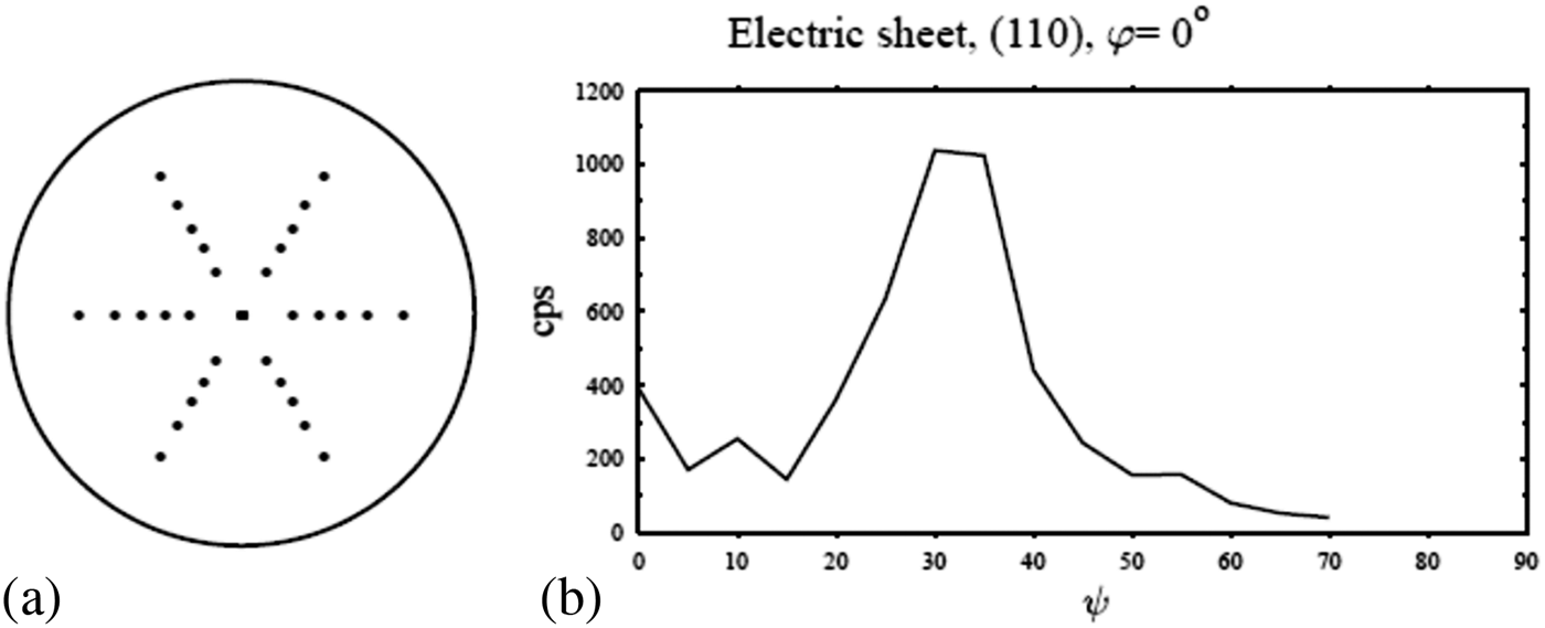
The difficulties arising from texture are twofold. One is the fact that the sin2ψ method is not appropriate because usually the lattice plane distances do not linearly depend on sin2ψ. The other problem with texture very often is this: in the traditional sin2ψ it is necessary to distribute the measurement direction as shown for example in the stereographic plot of Figure 1(a). The point of matter is to get sufficiently long and dense chains of accurately measured d-values at constant azimuths φ. In a textured material, this is often impossible as can be seen in the example of Figure 1(b). The intensity and the signal to background ratio must be high enough in order to obtain accurate 2θ and d values. Because of the intensity distribution as in Figure 1(b), good accuracy can only be expected in the range of about ψ = 20° to 45°.

Figure 1 (a) Possible arrangemnt of measurement directions suited the traditional sin2ψ method. (b) Dependence of peak intensities on ψ, along φ = 0°, due to strong texture.
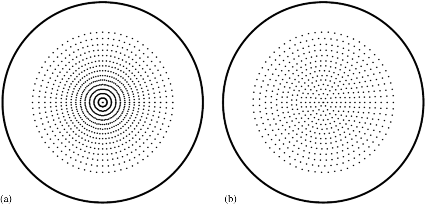
In our method, one is not restricted to these traditional distributions of φ/ψ but can use any distribution of measurement points (φ/ψ), for instance those which are usually applied in pole figure measurements; see Figure 2(a). A more rational distribution with a nearly constant density of the measurement points [Figure 2(b)] (Tarkowski, Reference Tarkowski2004) would of course also be appropriate.

Figure 2. Different distributions of measurement directions for a textured material. (a) The most frequently used distribution with constant φ/ψ steps. (b) A more efficient distribution with a (nearly) homogeneous covering of the orientation sphere.
To cope with the nonlinearity we use the relationship between ε(φ,ψ) and σ ij as discovered by Dölle and Hauk (Reference Dölle1979), Dölle (Reference Dölle and Hauk1979), Hauk (Reference Hauk1997), or a relationship derived from it (see below). The problem of not always being able to measure at any φ/ψ pair (with φ = const) is solved simply by abolishing the traditional sin2ψ method and instead use a method we call either matrix method or generalized sin2ψ method (Ortner, Reference Ortner2009a, Reference Ortner2009b, Reference Ortner2011). Modern X-ray facilities play to that aim inasmuch as they are often equipped with a linear detector instead of a point detector. With such a detector each pole figure measurement [necessary for the calculation of the orientation distribution function (odf) and then the F-tensor] automatically yields also the 2θ position at a very great number of measurement directions (given by φ/ψ), densely distributed over nearly the whole orientation sphere.
The second problem we are addressing here is if the material to be probed consists of more than one phase. Then, each phase has its own s 1 and s 2 for each hkl (in the quasi-isotropic case) or its own sets of F ij(φ, ψ, hkl, phase-number). These problems are solved by using a recently developed new method (Ortner, to be published) to calculate the F ij tensor. And the quasi-isotropic case is simply dealt as a textured one, taking an odf for quasi-isotropy.
Our method does not cover the following cases: we do not deal explicitly with a gradient of the stress tensor or a gradient in composition. The method is per se also not applicable to tackle the case where extra residual stresses of second order are present, that is, second-order residual stresses because of plastic deformation.
II. EXPERIMENTAL
Measurements are done as they are usually done for texture measurement. That means: all three Eulerian angles in steps of 5°, φ 1 and φ 2 from 0° to 360°, and Φ at least from 0° to 70°. The number of different pole figure measurements must be sufficient for the calculation of the odf. For measurement of the reflected beam, we apply a linear detector. This detector is crucial for the method, since it provides us a full diffractogram at each of some hundreds of positions given by φ/χ.
III. THEORETICAL BASIS
The basic equation of the method is Dölle–Hauk's equation (Dölle and Hauk, Reference Dölle1979).
In this (original) form, it must be used when the full stress tensor is to be determined (Ortner, Reference Ortner2009a, Reference Ortner2009b, Reference Ortner2011). In our case, where we regard a sample with a stress-free surface Eq. (2) can be used, which is derived from Eq. (1) (Skrzypek et al., Reference Skrzypek, Baczmanski, Ratuszeka and Kusiorc2001; Baczmanski et al., Reference Baczmanski, Braham and Seiler2003; Ortner, Reference Ortner2009a, Reference Ortner2009b, Reference Ortner2011).
Here a(φ, ψ, hkl) is the measured lattice parameter, calculated from the measured lattice plane distance d(φ, ψ, hkl).
where g ij is the contravariant metric tensor of the crystal lattice.
F ij (φ, ψ, hkl) are the components of the second rank tensor, frequently called X-ray elastic factors or X-ray stress factors. The calculation of the F-tensor is done with a completely new method (Ortner, to be published). For that new calculation method we decided to follow the Hill–Neerfeld approach. It would also be possible to use Kröner–Eshelby algorithm, but we do think that it doesn't make a great difference. Input data for this calculations are: the elastic property of the single crystal in the form of either S ij or C ij and a data file containing discrete values of the orientation distribution function, i.e. φ1, φ2, ϕ, f(g). If the material to be probed is a multiphase one then S ij or C ij must be known for each phase as well as the odfs and the volume fraction of each phase.
With enough measurements (here some hundreds of it) a system of linear equations can be establish which has to be solved for the unknowns a 0, a 0σ11, a 0a 22, a 0σ12. In this system of linear equations, it is absolutely mandatory to introduce weights for the different lines. This is because of the fact that all d-values obtained in a pole figure measurement are used, even those with small accuracy. The weights are inversely proportional to the standard deviations of the corresponding measurements. They are calculated using counting statistics and are functions of the peak height, the background level, the total number of counts and the peak line width. Since measurements with different (hkl)s can be used, the well-known tanθ dependence is also taken into account. For details of how to establish and solve the system of linear equations see for example Ortner (Reference Ortner2009a, Reference Ortner2009b, Reference Ortner2011) or any linear algebra textbook.
Remark: We want to point out here the fact that the method of stress calculation given in Eq. (2) has already been used and published by Skrzypek et al. (Reference Skrzypek, Baczmanski, Ratuszeka and Kusiorc2001) and Baczmanski et al. (Reference Baczmanski, Braham and Seiler2003) years before it was reinvented by one of the authors (B. O.) of the present paper. He, as well as the coauthors unfortunately missed these publications for a long time.
IV. ERROR ESTIMATION
Standard deviations for σ ij are calculated in the usual way, that is with the formula:
where Δa refers to the standard deviation of the measured lattice constant and p i to the weight of the ith measurement; n is the total number of measurements at φ/ψ, m is the number of unknowns (m = 4). From Δa one can calculate Δa 0 and Δσ ij as well as the standard deviations for all stresses derived from the stress tensor, which are the deviatoric stress σ′ij, the principal stresses σ 1, σ 11, σ 111, the von Mises stress and the Tresca stress. However, it must be pointed out, this algorithm, which is meant not for hundreds of measured data but instead for a handful or dozens of it produces rather unrealistically small standard deviations. They have to be taken with care and further considerations about error calculation seem to be necessary in that special case.
V. REPRESENTATION OF RESULTS
In the sin2ψ method, the plot of a versus sin2ψ provides us with a means to get an intuitive sense of the quality of the whole stress measurement. One can directly see how strong or how little the measured and the recalculated lattice plane distances (regression line) differ from each other. With the new method we do virtually the same but the measured data a(φ, ψ, hkl) – only those with the same φ must be taken – are not compared with a straight line but instead with the recalculated value of a. Of course, if the material is a quasi-isotropic one the recalculated values give a straight line. Such φ = constant – plots can be done for any φ. Yet they all have the disadvantage that only a rather small section of the whole data field would be depicted.
We therefore invented a new kind of data plotting, a method which aims to resemble the traditional sin2ψ plot. For that plot, we use as the abscissa either the 11- or the 22-component of the F-tensor. The depicted quantity is called a′. For the F 11 plot, a′ is defined in Eq. (5). For the F 22 plot, a′ is defined analogously with indices 22 instead of 11.
The idea behind this equation and the plot is obvious: if the measured value of a(φ, ψ, hkl) is equal to the recalculated one, as it would be in an ideal measurement, then only the third term of the right-hand side of Eq. (5) would be left over and all measured points would lie on a straight line. An F 11 plot is shown in Figure 3.

Figure 3. (Color online) Schematic diagram of stress evaluation for a multiphase, textured material.
A. Implementation of the method
All the above mentioned procedures and formulae are options, implemented in the program package “Rayflex StressOr” of GE Sensing & Inspection Technologies, SEIFERT Analytical X-rays.
In Figure 4, the whole procedure of an X-ray or neutron diffraction stress measurement for a multiphase and textured material, the most difficult case, is shown in the graphical form.

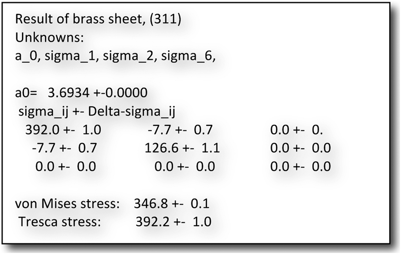
Figure 4. Example of a printed result.
B. An example
To test our method, a sheet of cold rolled brass (CuZn38, 1 mm thick) with a pronounced texture was set under an applied stress in a bending apparatus and underwent the above described measurement and data evaluation procedure. To eliminate the effect of extra second-order stresses we did two measurements, one without applied stress (no bending of the specimen) and one with stress. The data of both measurements have been subtracted so that only the effect of the applied stress is taken into account.
The X-ray equipment used was a GE Seifert Charon XRD with a Meteor1D detector. The radiation used was CoKα.
Pole figures were measured at (111), (200), (311), (220), and (400), the first four of these pole figures were used for the odf calculation. The F-tensors was calculated with the newly developed method.
In Figure 5, the numerical results are shown. Figure 6 shows two different sin2ψ plots and Figure 3 the F 11 plot, where the distance between the measured and recalculated values can be seen for all the 1094 measured points.

Figure 5. (Color online) sin2ψ plots of measured and recalculated lattice parameters (a) showing the nonlinearity due to strong texture.

Figure 6. (Color online) a′(φ, ψ, hkl) plotted versus F 11(φ, ψ, hkl). For the definition of a′ see Eq. (5) and text.


