1 Introduction
Stuart vortices are well-known exact solutions of the steady two-dimensional Euler equation in an unbounded planar domain characterized by a smooth and non-vanishing distribution of vorticity (Newton Reference Newton2001). The solution was derived by Stuart (Reference Stuart1967), who posed an exponential relationship between the stream function and the vorticity, thereby leading to consideration of the elliptic Liouville partial differential equation. On writing down a particular explicit solution of this partial differential equation, Stuart found that, as a parameter in his solution is varied from 1 to
 $\infty$
, the corresponding velocity field varies from a
$\infty$
, the corresponding velocity field varies from a
 $\tanh$
profile that models a laminar shear layer, to a single periodic row of point vortices. As such, the class of Stuart vortices are generally viewed as a smoothed version, or desingularization, of a periodic row of point vortices.
$\tanh$
profile that models a laminar shear layer, to a single periodic row of point vortices. As such, the class of Stuart vortices are generally viewed as a smoothed version, or desingularization, of a periodic row of point vortices.
Being among the few known analytical solutions of the steady Euler equation, Stuart’s solution has subsequently been generalized in several directions. Whereas the vorticity field of the Stuart solution has the same sign everywhere (co-rotating vortices), single rows of vortices of alternating signs (counter-rotating vortices) were found by Mallier & Maslowe (Reference Mallier and Maslowe1993), who posed that the vorticity is related to the stream function via a hyperbolic sine function. An attempt has been made to extend the Stuart model to the surface of a cylinder (Haslam & Mallier Reference Haslam and Mallier2003), although the validity of that solution has been questioned (Shusser Reference Shusser2004). Motivated by geophysical and astrophysical applications, Crowdy (Reference Crowdy2004) combined stereographic projection techniques with the methods of complex analysis to generalize the Stuart-vortex solution to the surface of a stationary sphere. The latter solutions, which are also expressible in closed form, describe smooth ‘cat’s-eye’ rings of
 $N\geqslant 2$
vortices around a latitude circle with steady point vortices at the two spherical poles. Those solutions have recently been generalized to a toroidal surface by Sakajo (Reference Sakajo2019). An analogous construction in the planar case (Crowdy Reference Crowdy2003) yields a single point vortex at the origin surrounded by an
$N\geqslant 2$
vortices around a latitude circle with steady point vortices at the two spherical poles. Those solutions have recently been generalized to a toroidal surface by Sakajo (Reference Sakajo2019). An analogous construction in the planar case (Crowdy Reference Crowdy2003) yields a single point vortex at the origin surrounded by an
 $N$
-polygonal ring of smooth vortices. Tur & Yanovsky (Reference Tur and Yanovsky2004) and Tur, Yanovsky & Kulik (Reference Tur, Yanovsky and Kulik2011) later contributed other aspects based on this idea. The solutions just described have been applied in a variety of contexts. Stuart vortices were used to study mixing layers in geophysical flows using a beta-plane model by Mallier (Reference Mallier1995). More recently, they have been used by Constantin & Krishnamurthy (Reference Constantin and Krishnamurthy2019) to model ocean gyres in spherical coordinates. Also, explicit solutions for compressible Stuart vortices in a homentropic gas flow were obtained for small Mach numbers via Rayleigh–Jansen expansions, and numerically studied for higher Mach numbers, in Meiron, Moore & Pullin (Reference Meiron, Moore and Pullin2000) and O’Reilly & Pullin (Reference O’Reilly and Pullin2003).
$N$
-polygonal ring of smooth vortices. Tur & Yanovsky (Reference Tur and Yanovsky2004) and Tur, Yanovsky & Kulik (Reference Tur, Yanovsky and Kulik2011) later contributed other aspects based on this idea. The solutions just described have been applied in a variety of contexts. Stuart vortices were used to study mixing layers in geophysical flows using a beta-plane model by Mallier (Reference Mallier1995). More recently, they have been used by Constantin & Krishnamurthy (Reference Constantin and Krishnamurthy2019) to model ocean gyres in spherical coordinates. Also, explicit solutions for compressible Stuart vortices in a homentropic gas flow were obtained for small Mach numbers via Rayleigh–Jansen expansions, and numerically studied for higher Mach numbers, in Meiron, Moore & Pullin (Reference Meiron, Moore and Pullin2000) and O’Reilly & Pullin (Reference O’Reilly and Pullin2003).
Crowdy (Reference Crowdy2003) mentions the possibility of generalizing his ‘hybrid’ solutions to other global equilibria comprising a more general distribution of stationary point vortices embedded in a smooth sea of Stuart-type vorticity. The present paper appears to be the first to identify non-trivial solutions of this kind: here we embed a pair of equal-circulation point vortices in a smooth sea of Stuart-type vorticity in such a way that the entire configuration, including the point vortices, is in equilibrium. Remarkably, we also show that there is a sense in which the new solutions here are a continuous extrapolation of the solutions of Crowdy (Reference Crowdy2003). The stationarity of the central point vortex at the origin in Crowdy’s solutions was easily argued on the basis of a rotational symmetry of the associated velocity field about the origin. By contrast, in the new solutions presented herein, the stationarity of the point vortices involves a more subtle interplay between the point vortices and the smooth Stuart-type vorticity in which they are embedded. We believe the fact that analytical solutions of the Euler equation exist within this hybrid class of what we refer to as ‘Stuart-embedded point vortex equilibria’ is of some theoretical significance.
The new hybrid solutions also have intriguing limits in which the Stuart-type vorticity becomes localized, or concentrated, into additional point vortices. This is of particular interest because, in one such limit, those limiting solutions are found to constitute a smoothly deformable two-real-parameter family of point vortex equilibria whose complex potential can be written down in closed form.
2 Point vortices and Stuart vortices
Let us first review the notion of a point vortex, and the class of Stuart vortices. The two-dimensional, incompressible flow of an inviscid homogeneous fluid is governed by the law of conservation of momentum, written in the form of the Euler equation (Saffman Reference Saffman1992)
 $$\begin{eqnarray}\frac{\unicode[STIX]{x2202}\boldsymbol{V}}{\unicode[STIX]{x2202}t}+(\boldsymbol{V}\boldsymbol{\cdot }\unicode[STIX]{x1D735})\boldsymbol{V}=-\frac{\unicode[STIX]{x1D735}p}{\unicode[STIX]{x1D70C}_{0}}.\end{eqnarray}$$
Here
 $\boldsymbol{V}(x,y)$
is the velocity field with Cartesian components
$\boldsymbol{V}(x,y)$
is the velocity field with Cartesian components
 $\boldsymbol{V}=(u,v)$
,
$\boldsymbol{V}=(u,v)$
,
 $(x,y)$
are the Cartesian coordinates of a planar cross-section of the flow,
$(x,y)$
are the Cartesian coordinates of a planar cross-section of the flow,
 $\unicode[STIX]{x1D735}$
is the two-dimensional gradient operator,
$\unicode[STIX]{x1D735}$
is the two-dimensional gradient operator,
 $p(x,y)$
is the pressure and
$p(x,y)$
is the pressure and
 $\unicode[STIX]{x1D70C}_{0}$
is the constant density of the fluid. In two-dimensional flow, the vorticity
$\unicode[STIX]{x1D70C}_{0}$
is the constant density of the fluid. In two-dimensional flow, the vorticity
 $\unicode[STIX]{x1D74E}=\unicode[STIX]{x1D735}\times \boldsymbol{V}$
has a single non-zero component
$\unicode[STIX]{x1D74E}=\unicode[STIX]{x1D735}\times \boldsymbol{V}$
has a single non-zero component
 $$\begin{eqnarray}\unicode[STIX]{x1D701}=\frac{\unicode[STIX]{x2202}v}{\unicode[STIX]{x2202}x}-\frac{\unicode[STIX]{x2202}u}{\unicode[STIX]{x2202}y}\end{eqnarray}$$
satisfying the vorticity equation (Saffman Reference Saffman1992)
 $$\begin{eqnarray}\frac{\unicode[STIX]{x2202}\unicode[STIX]{x1D701}}{\unicode[STIX]{x2202}t}+u\frac{\unicode[STIX]{x2202}\unicode[STIX]{x1D701}}{\unicode[STIX]{x2202}x}+v\frac{\unicode[STIX]{x2202}\unicode[STIX]{x1D701}}{\unicode[STIX]{x2202}y}=0.\end{eqnarray}$$
Conservation of mass requires that
 $\unicode[STIX]{x1D735}\boldsymbol{\cdot }\boldsymbol{V}=0$
(Saffman Reference Saffman1992), allowing us to define a stream function
$\unicode[STIX]{x1D735}\boldsymbol{\cdot }\boldsymbol{V}=0$
(Saffman Reference Saffman1992), allowing us to define a stream function
 $\unicode[STIX]{x1D713}(x,y)$
via
$\unicode[STIX]{x1D713}(x,y)$
via
 $$\begin{eqnarray}u=\frac{\unicode[STIX]{x2202}\unicode[STIX]{x1D713}}{\unicode[STIX]{x2202}y}\quad \text{and}\quad v=-\frac{\unicode[STIX]{x2202}\unicode[STIX]{x1D713}}{\unicode[STIX]{x2202}x}.\end{eqnarray}$$
In terms of the stream function, the vorticity given by (2.2) can be written as
 $$\begin{eqnarray}\unicode[STIX]{x1D701}=-\unicode[STIX]{x1D6FB}^{2}\unicode[STIX]{x1D713},\end{eqnarray}$$
where
 $\unicode[STIX]{x1D6FB}^{2}=\unicode[STIX]{x2202}^{2}/\unicode[STIX]{x2202}x^{2}+\unicode[STIX]{x2202}^{2}/\unicode[STIX]{x2202}y^{2}$
is the two-dimensional Laplacian. The vorticity equation (2.3) therefore becomes
$\unicode[STIX]{x1D6FB}^{2}=\unicode[STIX]{x2202}^{2}/\unicode[STIX]{x2202}x^{2}+\unicode[STIX]{x2202}^{2}/\unicode[STIX]{x2202}y^{2}$
is the two-dimensional Laplacian. The vorticity equation (2.3) therefore becomes
 $$\begin{eqnarray}\frac{\unicode[STIX]{x2202}(\unicode[STIX]{x1D6FB}^{2}\unicode[STIX]{x1D713})}{\unicode[STIX]{x2202}t}+\frac{\unicode[STIX]{x2202}\unicode[STIX]{x1D713}}{\unicode[STIX]{x2202}y}\frac{\unicode[STIX]{x2202}(\unicode[STIX]{x1D6FB}^{2}\unicode[STIX]{x1D713})}{\unicode[STIX]{x2202}x}-\frac{\unicode[STIX]{x2202}\unicode[STIX]{x1D713}}{\unicode[STIX]{x2202}x}\frac{\unicode[STIX]{x2202}(\unicode[STIX]{x1D6FB}^{2}\unicode[STIX]{x1D713})}{\unicode[STIX]{x2202}y}=0.\end{eqnarray}$$
2.1 Point vortices
Let us define the complex flow plane
 $z=x+\text{i}y$
and make the formal change of variables
$z=x+\text{i}y$
and make the formal change of variables
 $(x,y)\mapsto (z,\bar{z})$
, where
$(x,y)\mapsto (z,\bar{z})$
, where
 $\bar{z}=x-\text{i}y$
and overbars denote complex conjugates. Point vortex solutions to the Euler equation are obtained by solving the Poisson equation (2.5) with the source vorticity
$\bar{z}=x-\text{i}y$
and overbars denote complex conjugates. Point vortex solutions to the Euler equation are obtained by solving the Poisson equation (2.5) with the source vorticity
 $\unicode[STIX]{x1D701}$
consisting of a sum of
$\unicode[STIX]{x1D701}$
consisting of a sum of
 $M$
Dirac delta distributions (Newton Reference Newton2001),
$M$
Dirac delta distributions (Newton Reference Newton2001),
 $$\begin{eqnarray}\unicode[STIX]{x1D701}=\mathop{\sum }_{k=1}^{M}\unicode[STIX]{x1D6E4}_{k}\unicode[STIX]{x1D6FF}(z-z_{k}).\end{eqnarray}$$
Here
 $z_{1},z_{2},\ldots ,z_{M}$
are the time-dependent locations of the point vortices and the constants
$z_{1},z_{2},\ldots ,z_{M}$
are the time-dependent locations of the point vortices and the constants
 $\unicode[STIX]{x1D6E4}_{1},\unicode[STIX]{x1D6E4}_{2},\ldots ,\unicode[STIX]{x1D6E4}_{M}$
are the circulations or strengths of the point vortices. The stream function for the point vortex flow is given by
$\unicode[STIX]{x1D6E4}_{1},\unicode[STIX]{x1D6E4}_{2},\ldots ,\unicode[STIX]{x1D6E4}_{M}$
are the circulations or strengths of the point vortices. The stream function for the point vortex flow is given by
 $$\begin{eqnarray}\unicode[STIX]{x1D713}(z,\bar{z})=-\frac{1}{2\unicode[STIX]{x03C0}}\mathop{\sum }_{k=1}^{M}\unicode[STIX]{x1D6E4}_{k}\log |z-z_{k}|,\end{eqnarray}$$
and is the imaginary part of the complex potential
 $$\begin{eqnarray}f(z)=\frac{1}{2\unicode[STIX]{x03C0}\text{i}}\mathop{\sum }_{k=1}^{M}\unicode[STIX]{x1D6E4}_{k}\log (z-z_{k}).\end{eqnarray}$$
The velocity field is given in terms of the complex potential by
 $$\begin{eqnarray}u-\text{i}v=f^{\prime }(z)=\frac{1}{2\unicode[STIX]{x03C0}\text{i}}\mathop{\sum }_{k=1}^{M}\frac{\unicode[STIX]{x1D6E4}_{k}}{z-z_{k}},\end{eqnarray}$$
where primes denote derivatives with respect to the argument. Like the complex potential, the complex velocity
 $u-\text{i}v$
is a complex analytic function of
$u-\text{i}v$
is a complex analytic function of
 $z$
alone (independent of
$z$
alone (independent of
 $\bar{z}$
). The velocity of a point vortex is found by subtracting off the infinite self-induced term from (2.10) (Saffman Reference Saffman1992; Newton Reference Newton2001):
$\bar{z}$
). The velocity of a point vortex is found by subtracting off the infinite self-induced term from (2.10) (Saffman Reference Saffman1992; Newton Reference Newton2001):
 $$\begin{eqnarray}\overline{\frac{\text{d}z_{k}}{\text{d}t}}=\left.\left[(u-\text{i}v)-\frac{\unicode[STIX]{x1D6E4}_{k}}{2\unicode[STIX]{x03C0}\text{i}}\frac{1}{z-z_{k}}\right]\right|_{z=z_{k}}=\frac{1}{2\unicode[STIX]{x03C0}\text{i}}\mathop{\sum }_{\frac{j=1}{j\neq k}}^{M}\frac{\unicode[STIX]{x1D6E4}_{j}}{z_{k}-z_{j}},\end{eqnarray}$$
for
 $k=1,2,\ldots ,M$
. Equations (2.10) and (2.11) guarantee that (2.3) is solved in a weak sense.
$k=1,2,\ldots ,M$
. Equations (2.10) and (2.11) guarantee that (2.3) is solved in a weak sense.
2.2 Stuart vortices
Smooth steady solutions to the vorticity equation (2.6) can be obtained by solving
 $$\begin{eqnarray}\unicode[STIX]{x1D6FB}^{2}\unicode[STIX]{x1D713}=F(\unicode[STIX]{x1D713}),\end{eqnarray}$$
where we have the freedom to choose the differentiable function
 $F$
and hence the vorticity
$F$
and hence the vorticity
 $\unicode[STIX]{x1D701}$
in (2.5). Stuart (Reference Stuart1967) made the choice
$\unicode[STIX]{x1D701}$
in (2.5). Stuart (Reference Stuart1967) made the choice
 $$\begin{eqnarray}F(\unicode[STIX]{x1D713})=a\exp (b\unicode[STIX]{x1D713})\end{eqnarray}$$
for some real constants
 $a$
and
$a$
and
 $b$
so that (2.12) becomes a Liouville equation
$b$
so that (2.12) becomes a Liouville equation
 $$\begin{eqnarray}\unicode[STIX]{x1D6FB}^{2}\unicode[STIX]{x1D713}=a\exp (b\unicode[STIX]{x1D713}).\end{eqnarray}$$
The general solution to the Liouville equation (2.14) is known (Crowdy Reference Crowdy1997) to be expressible in terms of an analytic function
 $h(z)$
as
$h(z)$
as
 $$\begin{eqnarray}\unicode[STIX]{x1D713}(z,\bar{z})=\frac{1}{b}\log \left[\frac{2|h^{\prime }(z)|^{2}}{-ab(1+|h(z)|^{2})^{2}}\right].\end{eqnarray}$$
Stuart’s original solution corresponds to the choice (Stuart Reference Stuart1967)
 $$\begin{eqnarray}h(z)=A\tan \left(\frac{z}{2}\right)\quad \;\Longrightarrow \;\quad h^{\prime }(z)=\frac{A}{2}\sec ^{2}\left(\frac{z}{2}\right),\end{eqnarray}$$
where
 $A$
is a non-zero constant. This choice gives rise to the so-called planar Stuart-vortex solution described in the Introduction. We see from (2.16) that
$A$
is a non-zero constant. This choice gives rise to the so-called planar Stuart-vortex solution described in the Introduction. We see from (2.16) that
 $h^{\prime }(z)$
, and hence the argument of the logarithm in (2.15) does not vanish anywhere in the complex plane. The resulting velocity and vorticity fields are therefore everywhere smooth.
$h^{\prime }(z)$
, and hence the argument of the logarithm in (2.15) does not vanish anywhere in the complex plane. The resulting velocity and vorticity fields are therefore everywhere smooth.
The relations (2.4) can be combined to obtain an expression for the complex velocity field
 $u-\text{i}v$
in terms of the stream function
$u-\text{i}v$
in terms of the stream function
 $\unicode[STIX]{x1D713}(z,\bar{z})$
as
$\unicode[STIX]{x1D713}(z,\bar{z})$
as
 $$\begin{eqnarray}u-\text{i}v=2\text{i}\frac{\unicode[STIX]{x2202}\unicode[STIX]{x1D713}}{\unicode[STIX]{x2202}z}.\end{eqnarray}$$
On substitution of (2.15), we find that the velocity field associated with the Stuart-vortex solution is, in terms of the analytic function
 $h(z)$
,
$h(z)$
,
 $$\begin{eqnarray}u-\text{i}v=\frac{2\text{i}}{b}\left[\frac{h^{\prime \prime }(z)}{h^{\prime }(z)}-\frac{2h^{\prime }(z)}{h(z)}\frac{|h(z)|^{2}}{1+|h(z)|^{2}}\right].\end{eqnarray}$$
3 Stuart-embedded point vortex equilibria
For
 $\unicode[STIX]{x1D713}(z,\bar{z})$
in (2.15) to be regular, the function
$\unicode[STIX]{x1D713}(z,\bar{z})$
in (2.15) to be regular, the function
 $h^{\prime }(z)$
must not have any zeros in the domain (Crowdy Reference Crowdy2003). On the other hand if we choose
$h^{\prime }(z)$
must not have any zeros in the domain (Crowdy Reference Crowdy2003). On the other hand if we choose
 $$\begin{eqnarray}h^{\prime }(z)=2Az\quad \;\Longrightarrow \;\quad h(z)=Az^{2}+B,\end{eqnarray}$$
where
 $A$
and
$A$
and
 $B$
are constants, then we see that near
$B$
are constants, then we see that near
 $z=0$
the stream function looks like
$z=0$
the stream function looks like
 $$\begin{eqnarray}\unicode[STIX]{x1D713}(z,\bar{z})=\frac{2}{b}\log |z|+\text{regular function}.\end{eqnarray}$$
Although the solution is no longer regular at
 $z=0$
, this is nevertheless a physically acceptable form of singularity: indeed, on comparing (3.2) with (2.8), we see that this singular term corresponds to a point vortex of strength
$z=0$
, this is nevertheless a physically acceptable form of singularity: indeed, on comparing (3.2) with (2.8), we see that this singular term corresponds to a point vortex of strength
 $\unicode[STIX]{x1D6E4}=-4\unicode[STIX]{x03C0}/b$
at
$\unicode[STIX]{x1D6E4}=-4\unicode[STIX]{x03C0}/b$
at
 $z=0$
. Due to a symmetry of the associated velocity field (2.18) about the origin (notice that
$z=0$
. Due to a symmetry of the associated velocity field (2.18) about the origin (notice that
 $u-\text{i}v\mapsto -(u-\text{i}v)$
as
$u-\text{i}v\mapsto -(u-\text{i}v)$
as
 $z\mapsto -z$
), the non-self-induced velocity of the point vortex at the origin is zero (see (2.11) or (3.7) below) and the point vortex is in equilibrium. The form (3.1) is the special case with
$z\mapsto -z$
), the non-self-induced velocity of the point vortex at the origin is zero (see (2.11) or (3.7) below) and the point vortex is in equilibrium. The form (3.1) is the special case with
 $N=2$
of the more general choice
$N=2$
of the more general choice
 $$\begin{eqnarray}h(z)=Az^{N}+B\end{eqnarray}$$
considered by Crowdy (Reference Crowdy2003), where
 $A$
is a constant and
$A$
is a constant and
 $N\geqslant 2$
is an integer. For
$N\geqslant 2$
is an integer. For
 $B\neq 0$
the associated solution corresponds to a single point vortex at the origin, surrounded by an
$B\neq 0$
the associated solution corresponds to a single point vortex at the origin, surrounded by an
 $N$
-fold symmetric necklace of smooth Stuart-type vortices. Figure 1 shows streamline distributions for two different choices of the parameter
$N$
-fold symmetric necklace of smooth Stuart-type vortices. Figure 1 shows streamline distributions for two different choices of the parameter
 $B$
; the topology of the flow changes depending on whether
$B$
; the topology of the flow changes depending on whether
 $B$
is zero or non-zero. The streamlines are algebraic curves obtained from (2.15) to be
$B$
is zero or non-zero. The streamlines are algebraic curves obtained from (2.15) to be
 $$\begin{eqnarray}|z|^{2}=\unicode[STIX]{x1D6FC}(\unicode[STIX]{x1D713})\left(1+\left|\frac{z^{2}}{2}+B\right|^{2}\right)^{2},\end{eqnarray}$$
where the constant
 $\unicode[STIX]{x1D6FC}(\unicode[STIX]{x1D713})$
parametrizes the level sets of the stream function
$\unicode[STIX]{x1D6FC}(\unicode[STIX]{x1D713})$
parametrizes the level sets of the stream function
 $\unicode[STIX]{x1D713}$
.
$\unicode[STIX]{x1D713}$
.
Crowdy (Reference Crowdy2003) also showed that in the limit
 $A\rightarrow \infty$
the Stuart-type vorticity becomes localized into
$A\rightarrow \infty$
the Stuart-type vorticity becomes localized into
 $N$
additional satellite point vortices. The resulting pure point vortex equilibria correspond to those studied by Morikawa & Swenson (Reference Morikawa and Swenson1971), in which a central point vortex is surrounded by an
$N$
additional satellite point vortices. The resulting pure point vortex equilibria correspond to those studied by Morikawa & Swenson (Reference Morikawa and Swenson1971), in which a central point vortex is surrounded by an
 $N$
-fold symmetric array of satellite point vortices and such that the circulation of the central point vortex cancels out any net rotation of the polygonal ring of vortices about the central vortex. The analogous limit of the original Stuart-vortex solution (Stuart Reference Stuart1967) yields the single periodic point vortex row.
$N$
-fold symmetric array of satellite point vortices and such that the circulation of the central point vortex cancels out any net rotation of the polygonal ring of vortices about the central vortex. The analogous limit of the original Stuart-vortex solution (Stuart Reference Stuart1967) yields the single periodic point vortex row.

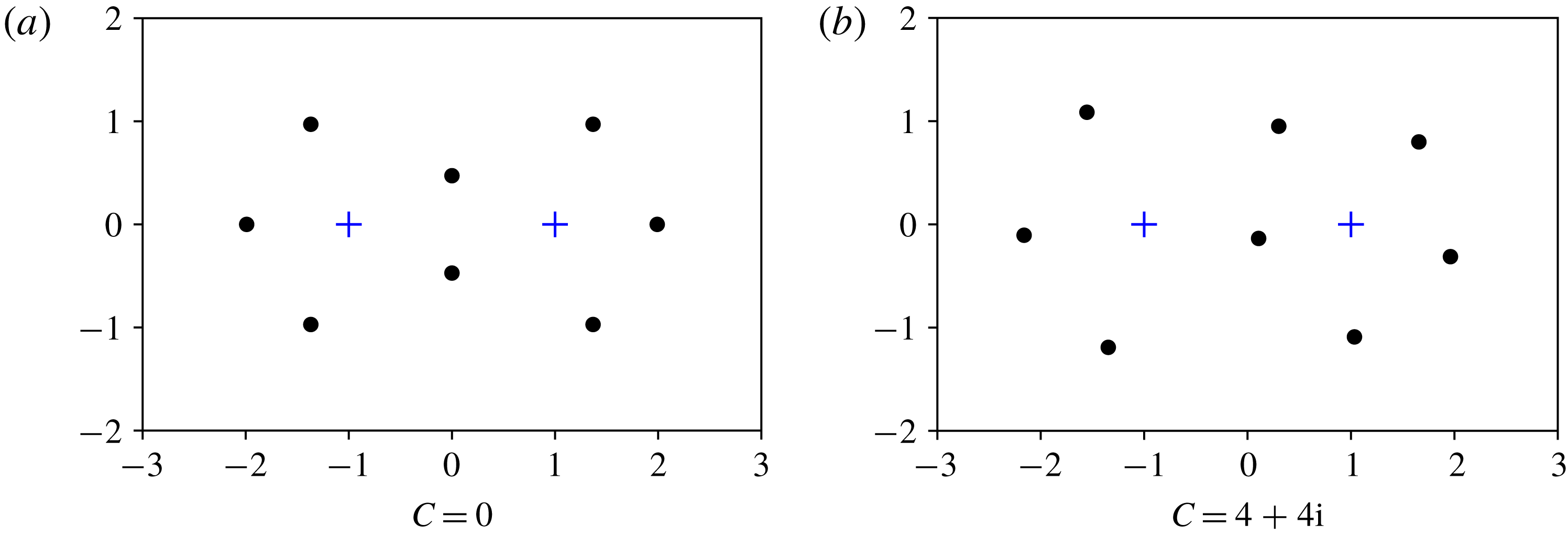
Figure 1. The
 $N=2$
solution of Crowdy (Reference Crowdy2003) obtained by inserting (3.1) into (2.15). A single central point vortex, marked by a blue
$N=2$
solution of Crowdy (Reference Crowdy2003) obtained by inserting (3.1) into (2.15). A single central point vortex, marked by a blue
 $+$
, has positive circulation, and is surrounded by a sea of negative smooth Stuart-type vorticity. The topology of the flow depends on the integration constant
$+$
, has positive circulation, and is surrounded by a sea of negative smooth Stuart-type vorticity. The topology of the flow depends on the integration constant
 $B$
. If
$B$
. If
 $B=0$
, the flow is rotationally symmetric about the origin, flowing counterclockwise near the point vortex and clockwise outside of the dashed red line. Taking
$B=0$
, the flow is rotationally symmetric about the origin, flowing counterclockwise near the point vortex and clockwise outside of the dashed red line. Taking
 $B=1$
breaks the rotational symmetry, and introduces two centres (‘smooth vortices’) along the
$B=1$
breaks the rotational symmetry, and introduces two centres (‘smooth vortices’) along the
 $x$
axis and two saddle points along the
$x$
axis and two saddle points along the
 $y$
axis. The contour level for the red streamline has been adjusted slightly so that it passes exactly through the saddle points. In the limit
$y$
axis. The contour level for the red streamline has been adjusted slightly so that it passes exactly through the saddle points. In the limit
 $A\rightarrow \infty$
the configuration tends to a pure point vortex equilibrium with two equal-circulation point vortices symmetrically disposed about the central point vortex.
$A\rightarrow \infty$
the configuration tends to a pure point vortex equilibrium with two equal-circulation point vortices symmetrically disposed about the central point vortex.
The presence of a point vortex at
 $z=0$
in the above example means that we are no longer solving the Liouville equation (2.14) there. Indeed, near
$z=0$
in the above example means that we are no longer solving the Liouville equation (2.14) there. Indeed, near
 $z=0$
we have from (3.2) that
$z=0$
we have from (3.2) that
 $$\begin{eqnarray}\unicode[STIX]{x1D6FB}^{2}\unicode[STIX]{x1D713}=\frac{2}{b}\unicode[STIX]{x1D6FB}^{2}(\log |z|+\text{regular function})=\frac{4\unicode[STIX]{x03C0}}{b}\unicode[STIX]{x1D6FF}(z)+\text{regular function},\end{eqnarray}$$
as expected for a point vortex of strength
 $\unicode[STIX]{x1D6E4}=-4\unicode[STIX]{x03C0}/b$
. In fact,
$\unicode[STIX]{x1D6E4}=-4\unicode[STIX]{x03C0}/b$
. In fact,
 $\unicode[STIX]{x1D713}$
is a solution of the modified Liouville equation
$\unicode[STIX]{x1D713}$
is a solution of the modified Liouville equation
 $$\begin{eqnarray}\unicode[STIX]{x1D6FB}^{2}\unicode[STIX]{x1D713}=a\exp (b\unicode[STIX]{x1D713})-\mathop{\sum }_{k=1}^{M}\unicode[STIX]{x1D6E4}_{k}\unicode[STIX]{x1D6FF}(z-z_{k})\end{eqnarray}$$
in the special case
 $M=1$
with
$M=1$
with
 $z_{1}=0$
and
$z_{1}=0$
and
 $\unicode[STIX]{x1D6E4}_{1}=-4\unicode[STIX]{x03C0}/b$
.
$\unicode[STIX]{x1D6E4}_{1}=-4\unicode[STIX]{x03C0}/b$
.
It is natural to ask (Crowdy Reference Crowdy2003) if more general hybrid vortical equilibria satisfying (3.6) can be constructed. For
 $z\neq z_{k}$
, equation (3.6) can be solved by the Stuart stream function (2.15). To obtain a consistent global equilibrium of the steady Euler equations, it is necessary and sufficient that the point vortices are stationary; this is equivalent to the point vortices being free of any net force. In the same way as in (2.11), the non-self-induced velocity of the point vortices in the Stuart model is calculated from (2.18) using the formula (Goodman, Hou & Lowengrub Reference Goodman, Hou and Lowengrub1990)
$z\neq z_{k}$
, equation (3.6) can be solved by the Stuart stream function (2.15). To obtain a consistent global equilibrium of the steady Euler equations, it is necessary and sufficient that the point vortices are stationary; this is equivalent to the point vortices being free of any net force. In the same way as in (2.11), the non-self-induced velocity of the point vortices in the Stuart model is calculated from (2.18) using the formula (Goodman, Hou & Lowengrub Reference Goodman, Hou and Lowengrub1990)
 $$\begin{eqnarray}\overline{\frac{\text{d}z_{k}}{\text{d}t}}=\left.\left[(u-\text{i}v)-\frac{\unicode[STIX]{x1D6E4}_{k}}{2\unicode[STIX]{x03C0}\text{i}}\frac{1}{z-z_{k}}\right]\right|_{z=z_{k}}\end{eqnarray}$$
for
 $k=1,2,\ldots ,M$
, and we require this velocity to be zero for each point vortex.
$k=1,2,\ldots ,M$
, and we require this velocity to be zero for each point vortex.
We now derive a new non-trivial solution of this kind with
 $M=2$
corresponding to a Stuart-embedded point vortex pair. To do so, we now choose
$M=2$
corresponding to a Stuart-embedded point vortex pair. To do so, we now choose
 $$\begin{eqnarray}h^{\prime }(z)=A\tilde{h}^{\prime }(z),\quad \tilde{h}^{\prime }(z)\equiv \frac{(z-1)^{4}(z+1)^{4}}{z^{2}},\end{eqnarray}$$
where
 $A$
is a real constant leading, upon integration, to
$A$
is a real constant leading, upon integration, to
 $$\begin{eqnarray}h(z)=A\tilde{h}(z)+B,\quad \tilde{h}(z)=\frac{z^{7}}{7}-\frac{4z^{5}}{5}+2z^{3}-4z-\frac{1}{z},\end{eqnarray}$$
where
 $B$
is a complex constant of integration. This is clearly a generalization of (3.1) and, as in that case, any point vortices in the solution will appear at the zeros of
$B$
is a complex constant of integration. This is clearly a generalization of (3.1) and, as in that case, any point vortices in the solution will appear at the zeros of
 $h^{\prime }(z)$
. For convenience, we continue to use the same names
$h^{\prime }(z)$
. For convenience, we continue to use the same names
 $A$
and
$A$
and
 $B$
for the parameters in (3.9) as used in (3.1), with the implicit understanding that each of the different solutions has its own independent choice of
$B$
for the parameters in (3.9) as used in (3.1), with the implicit understanding that each of the different solutions has its own independent choice of
 $A$
and
$A$
and
 $B$
.
$B$
.
On substitution of the choice (3.9) for
 $h(z)$
into (2.18) we obtain an explicit formula for a single-valued velocity field dependent on the two parameters
$h(z)$
into (2.18) we obtain an explicit formula for a single-valued velocity field dependent on the two parameters
 $A$
and
$A$
and
 $B$
. This velocity field contains singular terms corresponding to two point vortices, at
$B$
. This velocity field contains singular terms corresponding to two point vortices, at
 $z=\pm 1$
, the two zeros of
$z=\pm 1$
, the two zeros of
 $h^{\prime }(z)$
. It is important to note that the simple pole of
$h^{\prime }(z)$
. It is important to note that the simple pole of
 $h(z)$
at
$h(z)$
at
 $z=0$
does not lead to a singularity in
$z=0$
does not lead to a singularity in
 $\unicode[STIX]{x1D713}$
. It remains to show that the point vortices at
$\unicode[STIX]{x1D713}$
. It remains to show that the point vortices at
 $\pm 1$
are stationary, as otherwise we do not have a global equilibrium of the Euler equation. This is accomplished by finding a local expansion of the complex velocity (2.18) near
$\pm 1$
are stationary, as otherwise we do not have a global equilibrium of the Euler equation. This is accomplished by finding a local expansion of the complex velocity (2.18) near
 $z=1$
and
$z=1$
and
 $z=-1$
(see appendix A):
$z=-1$
(see appendix A):
 $$\begin{eqnarray}u-\text{i}v=\left\{\begin{array}{@{}ll@{}}\displaystyle \frac{8\text{i}}{b}\frac{1}{z-1}+o(1),\quad & \text{near }z=1,\\ \displaystyle \frac{8\text{i}}{b}\frac{1}{z+1}+o(1),\quad & \text{near }z=-1.\end{array}\right.\end{eqnarray}$$
The fact that the regular terms in these local expansions vanish as
 $z\rightarrow \pm 1$
implies that the point vortices at these locations are in equilibrium. By comparison with (2.10), the two point vortices have equal circulation
$z\rightarrow \pm 1$
implies that the point vortices at these locations are in equilibrium. By comparison with (2.10), the two point vortices have equal circulation
 $\unicode[STIX]{x1D6E4}=-16\unicode[STIX]{x03C0}/b$
. Varying
$\unicode[STIX]{x1D6E4}=-16\unicode[STIX]{x03C0}/b$
. Varying
 $b$
simply shifts and rescales the stream function, as seen from (2.15), so we pick
$b$
simply shifts and rescales the stream function, as seen from (2.15), so we pick
 $b=-16\unicode[STIX]{x03C0}$
to normalize the point vortex circulations to
$b=-16\unicode[STIX]{x03C0}$
to normalize the point vortex circulations to
 $\unicode[STIX]{x1D6E4}=1$
. Since we require
$\unicode[STIX]{x1D6E4}=1$
. Since we require
 $ab<0$
(so that the argument of the logarithm in (2.15) is non-negative), it follows that
$ab<0$
(so that the argument of the logarithm in (2.15) is non-negative), it follows that
 $a>0$
, and hence from (2.13) and (2.5) that the Stuart-type vorticity contribution is everywhere negative.
$a>0$
, and hence from (2.13) and (2.5) that the Stuart-type vorticity contribution is everywhere negative.
It is well known that two point vortices of equal strength with the same sign, in otherwise irrotational flow, rotate with constant angular velocity about the midpoint of the line joining them (Newton Reference Newton2001). For the Stuart-embedded point vortex pair just found, the point vortices with positive strength are surrounded by a sea of smooth, negative Stuart-type vorticity, and it is this that keeps the point vortices stationary, yielding a global equilibrium of the Euler equation.

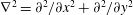
Figure 2. Streamlines for the Stuart-embedded point vortex pair with
 $A=1$
and different values of
$A=1$
and different values of
 $B$
. The two point vortices are marked by a
$B$
. The two point vortices are marked by a
 $+$
, and have equal circulation
$+$
, and have equal circulation
 $\unicode[STIX]{x1D6E4}=1$
. They are surrounded by a sea of negative Stuart vorticity which acts to render the point vortex pair stationary. (a)
$\unicode[STIX]{x1D6E4}=1$
. They are surrounded by a sea of negative Stuart vorticity which acts to render the point vortex pair stationary. (a)
 $B=0$
and the solution is symmetric around the two point vortices; (b) and (c) the symmetry is partially broken by choosing purely real or imaginary
$B=0$
and the solution is symmetric around the two point vortices; (b) and (c) the symmetry is partially broken by choosing purely real or imaginary
 $B$
; (d)
$B$
; (d)
 $B$
is complex and the solution is completely asymmetric.
$B$
is complex and the solution is completely asymmetric.
Typical streamline patterns for the Stuart-embedded point vortex pair are shown in figure 2. The streamlines are algebraic curves whose equations are
 $|h^{\prime }(z)|^{2}=\unicode[STIX]{x1D6FD}(\unicode[STIX]{x1D713})(1+|h(z)|^{2})^{2}$
, where the constant
$|h^{\prime }(z)|^{2}=\unicode[STIX]{x1D6FD}(\unicode[STIX]{x1D713})(1+|h(z)|^{2})^{2}$
, where the constant
 $\unicode[STIX]{x1D6FD}(\unicode[STIX]{x1D713})$
parametrizes the streamlines, and
$\unicode[STIX]{x1D6FD}(\unicode[STIX]{x1D713})$
parametrizes the streamlines, and
 $h^{\prime }(z)$
and
$h^{\prime }(z)$
and
 $h(z)$
are given by (3.8) and (3.9). At large distances from the Stuart-embedded point vortex pair the streamlines become circular to a first approximation.
$h(z)$
are given by (3.8) and (3.9). At large distances from the Stuart-embedded point vortex pair the streamlines become circular to a first approximation.
There are several interesting limiting cases of these solutions. As
 $A\rightarrow 0$
the stream function becomes unbounded, but inspection of the expression (2.18) for the velocity field shows that
$A\rightarrow 0$
the stream function becomes unbounded, but inspection of the expression (2.18) for the velocity field shows that
 $$\begin{eqnarray}u-\text{i}v\rightarrow \frac{2\text{i}}{b}\left[\frac{\tilde{h}^{\prime \prime }(z)}{\tilde{h}^{\prime }(z)}\right].\end{eqnarray}$$
The associated stream function can be determined by suitably regularizing the limit of
 $\unicode[STIX]{x1D713}$
as
$\unicode[STIX]{x1D713}$
as
 $A\rightarrow 0$
; see, for example, equation (3.12) below. On use of the expression (3.8) for
$A\rightarrow 0$
; see, for example, equation (3.12) below. On use of the expression (3.8) for
 $\tilde{h}^{\prime }(z)$
the velocity field (3.11) is seen to be that associated with the point vortex equilibrium comprising two unit-circulation point vortices at
$\tilde{h}^{\prime }(z)$
the velocity field (3.11) is seen to be that associated with the point vortex equilibrium comprising two unit-circulation point vortices at
 $\pm 1$
and a point vortex of circulation
$\pm 1$
and a point vortex of circulation
 $-1/2$
at the origin. This is precisely the same 3-point vortex equilibrium deriving from a limit of the solution of Crowdy (Reference Crowdy2003) in (3.1) discussed earlier (cf. figure 1). Note, however, the important distinction that in those earlier solutions it is the point vortex at the origin – denoted by the blue ‘
$-1/2$
at the origin. This is precisely the same 3-point vortex equilibrium deriving from a limit of the solution of Crowdy (Reference Crowdy2003) in (3.1) discussed earlier (cf. figure 1). Note, however, the important distinction that in those earlier solutions it is the point vortex at the origin – denoted by the blue ‘
 $+$
’ in figure 1 – that is always present and that the two satellite point vortices at
$+$
’ in figure 1 – that is always present and that the two satellite point vortices at
 $\pm 1$
only emerge in a limiting case (as
$\pm 1$
only emerge in a limiting case (as
 $A\rightarrow \infty$
in the solution corresponding to (3.1)). In the new solutions corresponding to the choice (3.9) the satellite point vortices are always present – denoted by the blue ‘
$A\rightarrow \infty$
in the solution corresponding to (3.1)). In the new solutions corresponding to the choice (3.9) the satellite point vortices are always present – denoted by the blue ‘
 $+$
’ in figure 3 – and it is the point vortex at the origin that only emerges in a limiting case (as
$+$
’ in figure 3 – and it is the point vortex at the origin that only emerges in a limiting case (as
 $A\rightarrow 0$
in the solutions corresponding to (3.9)).
$A\rightarrow 0$
in the solutions corresponding to (3.9)).
We also explore the limit
 $A\rightarrow \infty$
for the new solutions corresponding to (3.9). Motivated by the analysis of Crowdy (Reference Crowdy2003), who fixes the location of the centres of recirculation in his solutions and finds that
$A\rightarrow \infty$
for the new solutions corresponding to (3.9). Motivated by the analysis of Crowdy (Reference Crowdy2003), who fixes the location of the centres of recirculation in his solutions and finds that
 $B$
scales linearly with
$B$
scales linearly with
 $A$
as
$A$
as
 $A\rightarrow \infty$
(see his Figure 1), we take
$A\rightarrow \infty$
(see his Figure 1), we take
 $A\rightarrow \infty$
with
$A\rightarrow \infty$
with
 $B=AC$
, where
$B=AC$
, where
 $C$
is some fixed complex constant so that
$C$
is some fixed complex constant so that
 $B\rightarrow \infty$
also. Now we find
$B\rightarrow \infty$
also. Now we find
 $$\begin{eqnarray}\lim _{A\rightarrow \infty }\left(\unicode[STIX]{x1D713}+\frac{2}{b}\log |A|\right)=\frac{2}{b}\log \left|\frac{z^{2}\tilde{h}^{\prime }(z)}{(z(\tilde{h}(z)+C))^{2}}\right|.\end{eqnarray}$$
There are generically eight point vortices of circulation
 $-1/2$
now at the roots of the degree-8 polynomial
$-1/2$
now at the roots of the degree-8 polynomial
 $z(\tilde{h}(z)+C)$
, resulting in a two-real-parameter family of point vortex equilibria whose vortex locations are parametrized by the real and imaginary parts of
$z(\tilde{h}(z)+C)$
, resulting in a two-real-parameter family of point vortex equilibria whose vortex locations are parametrized by the real and imaginary parts of
 $C$
. Whatever their locations – and these must be found by finding the (generically simple) roots of the polynomial
$C$
. Whatever their locations – and these must be found by finding the (generically simple) roots of the polynomial
 $z(\tilde{h}(z)+C)$
– these eight new point vortices can be shown to be in equilibrium, as must be the case. This can be directly verified by a local analysis of the limiting velocity field derived from (3.12) near a typical zero
$z(\tilde{h}(z)+C)$
– these eight new point vortices can be shown to be in equilibrium, as must be the case. This can be directly verified by a local analysis of the limiting velocity field derived from (3.12) near a typical zero
 $z_{k}$
(for
$z_{k}$
(for
 $k=1,\ldots ,8$
) of
$k=1,\ldots ,8$
) of
 $z(\tilde{h}(z)+C)$
:
$z(\tilde{h}(z)+C)$
:
 $$\begin{eqnarray}u-\text{i}v=\frac{\text{i}}{4\unicode[STIX]{x03C0}(z-z_{k})}+o(1),\quad k=1,\ldots ,8,\end{eqnarray}$$
implying that all eight point vortices are indeed in equilibrium.


Interestingly, the class of point vortex equilibria just derived by this second limiting process happen to coincide with those identified, using completely different mathematical arguments, by Loutsenko (Reference Loutsenko2004). The polynomial
 $z(\tilde{h}(z)+C)$
is precisely the polynomial
$z(\tilde{h}(z)+C)$
is precisely the polynomial
 $p_{-2}(z)/7$
found by Loutsenko (Reference Loutsenko2004), with his parameters taken to be
$p_{-2}(z)/7$
found by Loutsenko (Reference Loutsenko2004), with his parameters taken to be
 $\unicode[STIX]{x1D70F}_{-1}=-1$
and
$\unicode[STIX]{x1D70F}_{-1}=-1$
and
 $t_{-2}=C$
. O’Neil (Reference O’Neil2006) has also given a construction of families of point vortex equilibria depending on a complex-valued parameter.
$t_{-2}=C$
. O’Neil (Reference O’Neil2006) has also given a construction of families of point vortex equilibria depending on a complex-valued parameter.
4 Discussion
A new family of exact solutions to the steady planar Euler equation has been derived. The solutions provide a class of hybrid equilibria comprising two point vortices of equal circulation embedded in a sea of smooth Stuart-type vorticity of opposite sign. Varying two parameters
 $A$
and
$A$
and
 $B$
in the class of solutions leads to flows with differing streamline patterns.
$B$
in the class of solutions leads to flows with differing streamline patterns.
Of particular interest are limits of the hybrid equilibria where the vorticity associated with the Stuart-vortex sea becomes localized into additional point vortices. Two unit-circulation point vortices at
 $\pm 1$
are present for any value of
$\pm 1$
are present for any value of
 $A$
, but as
$A$
, but as
 $A\rightarrow 0$
an additional point vortex of circulation
$A\rightarrow 0$
an additional point vortex of circulation
 $-1/2$
forms at the origin with irrotational flow everywhere else. As
$-1/2$
forms at the origin with irrotational flow everywhere else. As
 $A\rightarrow \infty$
, on the other hand, the solutions give rise to a two-real-parameter family of eight point vortices of circulation
$A\rightarrow \infty$
, on the other hand, the solutions give rise to a two-real-parameter family of eight point vortices of circulation
 $-1/2$
, with all the point vortices now surrounded by irrotational flow. It is therefore natural to view the intermediate hybrid solutions for
$-1/2$
, with all the point vortices now surrounded by irrotational flow. It is therefore natural to view the intermediate hybrid solutions for
 $0<A<\infty$
as continuously interpolating between these two limiting pure point vortex equilibria. At the same time we have shown that the
$0<A<\infty$
as continuously interpolating between these two limiting pure point vortex equilibria. At the same time we have shown that the
 $A\rightarrow 0$
limit of the new solutions here coincides with the point vortex equilibrium arising as a limit of the hybrid solutions of Crowdy (Reference Crowdy2003). It is therefore also natural to view the new hybrid solutions found here as continuously extrapolating Crowdy’s solutions.
$A\rightarrow 0$
limit of the new solutions here coincides with the point vortex equilibrium arising as a limit of the hybrid solutions of Crowdy (Reference Crowdy2003). It is therefore also natural to view the new hybrid solutions found here as continuously extrapolating Crowdy’s solutions.
Hybrid equilibria of this kind appear to provide a mechanism whereby a given point vortex equilibrium can be partially desingularized to produce a smoother global equilibrium that can itself eventually become singular again at isolated points to produce a different point vortex equilibrium. There appear to be chains of such point vortex equilibria connected in this way by the kind of hybrid equilibria exemplified here.
Indeed we report the solutions here as some of the simplest non-trivial examples available from a novel mathematical construction of such hybrid Stuart-embedded point vortex equilibria recently uncovered by the authors. This more general construction requires posing an Ansatz for
 $h^{\prime }(z)$
as a rational function akin to (3.8); strategic choices of this rational function yield generalizations of the new solutions found here. A full description of this new mathematical construction of vortex equilibria, and its connections to other areas of mathematical physics, is in preparation.
$h^{\prime }(z)$
as a rational function akin to (3.8); strategic choices of this rational function yield generalizations of the new solutions found here. A full description of this new mathematical construction of vortex equilibria, and its connections to other areas of mathematical physics, is in preparation.
Acknowledgements
This research was supported by the WWTF research grant MA16-009 (V.S.K.). We thank the reviewers for helpful comments on an earlier version of this manuscript.
Appendix A
First we evaluate some Laurent series required to find the velocity of the point vortices at
 $z=1$
and
$z=1$
and
 $z=-1$
. We have from (3.8) that
$z=-1$
. We have from (3.8) that
 $$\begin{eqnarray}\frac{h^{\prime \prime }(z)}{h^{\prime }(z)}=\frac{6z^{7}-16z^{5}+12z^{3}-2/z}{(z-1)^{4}(z+1)^{4}}=\frac{t_{1}(z)}{(z-1)^{4}}=\frac{t_{2}(z)}{(z+1)^{4}},\end{eqnarray}$$
where
 $$\begin{eqnarray}t_{1}(z)=\frac{6z^{7}-16z^{5}+12z^{3}-2/z}{(z+1)^{4}},\quad \text{and}\quad t_{2}(z)=\frac{6z^{7}-16z^{5}+12z^{3}-2/z}{(z-1)^{4}}.\end{eqnarray}$$
We see that
 $t_{1}(z)$
is regular at
$t_{1}(z)$
is regular at
 $z=1$
, its derivatives are calculated from (A 2) to be
$z=1$
, its derivatives are calculated from (A 2) to be
 $$\begin{eqnarray}t_{1}(1)=0,\quad t_{1}^{\prime }(1)=0,\quad t_{1}^{\prime \prime }(1)=0,\quad t_{1}^{\prime \prime \prime }(1)=24,\quad t_{1}^{\prime \prime \prime \prime }(1)=0.\end{eqnarray}$$
Substituting into (A 1) we find that the Laurent series for
 $h^{\prime \prime }(z)/h^{\prime }(z)$
near
$h^{\prime \prime }(z)/h^{\prime }(z)$
near
 $z=1$
is
$z=1$
is
 $$\begin{eqnarray}\frac{h^{\prime \prime }(z)}{h^{\prime }(z)}=\frac{4}{z-1}+O(z-1).\end{eqnarray}$$
It is to be noted that
 $t_{1}^{\prime \prime \prime \prime }(1)$
is the crucial term that needs to be zero in order that the point vortex at
$t_{1}^{\prime \prime \prime \prime }(1)$
is the crucial term that needs to be zero in order that the point vortex at
 $z=1$
is stationary. Similarly,
$z=1$
is stationary. Similarly,
 $t_{2}(z)$
is regular at
$t_{2}(z)$
is regular at
 $z=-1$
. The required derivatives can be read off from (A 3) using the symmetry property
$z=-1$
. The required derivatives can be read off from (A 3) using the symmetry property
 $t_{2}(z)=-t_{1}(-z)$
, and we get
$t_{2}(z)=-t_{1}(-z)$
, and we get
 $$\begin{eqnarray}t_{2}(z)=4(z+1)^{3}+O((z+1)^{5}),\end{eqnarray}$$
leading to the Laurent series
 $$\begin{eqnarray}\frac{h^{\prime \prime }(z)}{h^{\prime }(z)}=\frac{4}{z+1}+O(z+1),\end{eqnarray}$$
near
 $z=-1$
. It is also necessary to ensure that the non-analytic contribution to the local velocity field vanishes at
$z=-1$
. It is also necessary to ensure that the non-analytic contribution to the local velocity field vanishes at
 $z=\pm 1$
. This is the second term in the square bracket in the expression (2.18) for the velocity, namely,
$z=\pm 1$
. This is the second term in the square bracket in the expression (2.18) for the velocity, namely,
 $2\,h^{\prime }(z)\overline{h(z)}/(1+|h(z)|^{2})$
. However, this expression clearly vanishes at
$2\,h^{\prime }(z)\overline{h(z)}/(1+|h(z)|^{2})$
. However, this expression clearly vanishes at
 $z=\pm 1$
because
$z=\pm 1$
because
 $h^{\prime }(z)$
vanishes at these points while
$h^{\prime }(z)$
vanishes at these points while
 $h(z)$
is finite there.
$h(z)$
is finite there.