


Introduction
The spatial and temporal evolution of past Antarctic ice sheets has had a major influence on the development of polar ecosystems within ice-free regions of Antarctica. The cycle of advance and retreat of Antarctic ice sheets would have necessarily eradicated most terrestrial life during ice sheet maxima with recolonization following their retreat and possibly longer-term preservation of only a very small subset of flora and fauna (Adams et al. Reference Adams, Bardgett, Ayres, Wall, Aislabe, Bamforth, Bargagli, Cary, Cavacini, Connell, Convey, Fell, Frati, Hogg, Newsham, O’donnel, Russell, Seppelt and Stevens2006, Stevens et al. Reference Stevens, Greenslade, Hogg and Sunnucks2006, Convey & Stevens Reference Convey and Stevens2007, Convey et al. Reference Convey, Gibson, Hillenbrand, Hodgson, Pugh, Smellie and Stevens2008). On the assumption that major continental ice sheet advances, including the Last Glacial Maximum (LGM), overran ice-free habitats and coastal oases, most terrestrial life would have been wiped out, with the exception of sub-surface bacteria. On this basis, one can then postulate that there may be a relationship between the biodiversity of a glacial landscape and its glacial history. A few ice-free terrestrial environments, such as the McMurdo Dry Valleys region, have existed within the Transantarctic Mountains for up to 10–12 million years (Sugden et al. Reference Sugden, Bentley and Cofaigh2006), although many more are likely.
However, in order to investigate the idea of a correlation between ice sheet size and biodiversity, the large uncertainties in the extent and thickness of formerly expanded ice sheets (Bentley Reference Bentley1999), particularly at the LGM (Mackintosh et al. Reference Mackintosh, White, Fink, Gore, Pickard and Fanning2007) require attention. Computer models of the past behaviour of the Antarctic ice sheet based on glaciological, marine and physical inputs have provided conflicting pictures (Bentley Reference Bentley1999, Denton & Hughes Reference Denton and Hughes2002, Huybrechts Reference Huybrechts2002). Confounding these efforts is the scarcity of terrestrial evidence, particularly in East Antarctica, due to the limited number of coastal mountain ice-free regions and their lack of datable material, particularly for radiocarbon dating. In parallel with these modelling uncertainties, reductions in the calculated volumes of the Laurentide and Fennoscandian ice caps appear to account for only a portion of the observed ∼120 m rise in global sea level since LGM times.
In the absence of any direct and/or local evidence for the volume of ice in Antarctica at the global LGM, early estimates were mostly based on the difference between known sea level change, and the known (Northern Hemisphere) ice sheets (Nakada & Lambeck Reference Nakada and Lambeck1988). As more direct evidence from the continent becomes increasingly available, estimates of the volume of grounded ice in Antarctica at the LGM are becoming correspondingly much smaller, particularly in East Antarctica. While it is clear from grounding line studies (Conway et al. Reference Conway, Hall, Denton, Gades and Waddington1999) that there were significant expansions of the West Antarctic Ice Sheet (WAIS) in the Ross Sea region, investigations on the main East Antarctic Ice Sheet (EAIS) have indicated relatively small ice sheet increases during the LGM (Gore et al. Reference Gore, Rhodes, Augustinus, Leishman, Colhoun and Rees-Jones2001, Mackintosh et al. Reference Mackintosh, White, Fink, Gore, Pickard and Fanning2007). Similarly, isostatic rebound along the McMurdo Sound coast based on raised beach elevations (Butler Reference Butler1999) suggest minimal isostatic loading during the same period.
This paper provides new geological evidence of ice sheet extent and thickness over at least the past few hundred thousand, and perhaps the past two million years within a sector of the Transantarctic Mountains in order to better constrain computer model estimates of palaeo-ice sheet changes. We describe the glacial history based on new in situ cosmogenic nuclide exposure ages of an ice-free region in the Darwin Mountains on the edge of the Hatherton Glacier, referred to as the Lake Wellman area (Fig. 1). The location is one of the study sites along the Latitudinal Gradient Project of the Transantarctic Mountains (Howard-Williams et al. Reference Howard-Williams, Peterson, Lyons, Cattaneo-Vietti and Gordon2006). The set of 25 cosmogenic exposure ages of erratics collected along two altitudinal transects allows estimates of ice volume changes of the Hatherton Glacier which, at the spatial resolution examined here, constrains ice sheet models and provides input into the biogeographic and evolutionary history of the Darwin Mountains region. Previous work from the Lake Wellman area of the Transantarctic Mountains has been used to support a “big ice” view of Antarctic glacial expansion at the LGM (Denton & Hughes Reference Denton and Hughes2002). Our results have strong implications for the role of the Ross Ice Shelf in ice sheet volume calculations at the LGM.

Fig. 1 Regional map (left figure) showing the location of Lake Wellman within the Hatherton and Darwin glacial system which discharges into the Ross Ice Shelf. Inset (right figure) shows location of Hatherton Glacier region (small black rectangle) with respect to Dry Valleys region of the Transantarctic Mountains (red dot). Diamond Hill and Dubris Valley are other field sites targeted for cosmogenic exposure dating.
The Lake Wellman area
The Hatherton Glacier flows from the EAIS into the lower Darwin Glacier, which in turn discharges ice into the Ross Ice Shelf (Fig. 1). The Darwin–Hatherton system is an important outflow glacier system that connected the East and West Antarctic ice sheets during previous glacial maxima. The advance and retreat of the Hatherton is recorded in well-preserved glacial moraines that are found in numerous side entrant valleys of the Darwin Mountains along the length of the glacier. Ice-free cirques and valleys in the Darwin Mountains are cut into Palaeozoic sandstones of the Beacon Supergroup and thick dolerite sills of the Jurassic Ferrar Supergroup (Haskell et al. Reference Haskell, Kennett and Prebble1964). In the vicinity of Lake Wellman, a large currently ice-free area had previously been completely or partially covered by ice (Bockheim et al. Reference Bockheim, Wilson, Denton, Andersen and Stuiver1989) resulting in multiple drift sheets deposited by palaeo-advances of the Hatherton Glacier. These deposits were mapped in the late 1970s by Bockheim et al. (Reference Bockheim, Wilson, Denton, Andersen and Stuiver1989) who identified five drift sheets that occur discontinuously in the ice-free regions extending over an elevation range of about 800 m from the edge of Lake Wellman, which is at 845 m above sea level (m a.s.l.) (Fig. 2). From youngest to oldest, with increasing distance from the present day margins of Lake Wellman, these are: 1) Hatherton, 2) Britannia I, 3) Britannia II, 4) Danum, and 5) Isca.
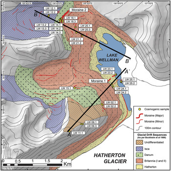
Fig. 2 A geomorphological map of the Lake Wellman area showing the distribution of the four main drift sequences after Bockheim et al. (Reference Bockheim, Wilson, Denton, Andersen and Stuiver1989). Black bold lines A–A′ and B–B′ represent altitudinal transects along which samples were collected from glacial deposits for exposure age dating. Sample sites are designated by rectangular boxes labelled as LW xx. Aerial photographs of moraines 1 and 2 are shown in Fig. 4. Hatherton Glacier ice flows from bottom-left to top-right in a direction semi-parallel to transect A–A′.
Currently, the altitude of the ice surface of the Hatherton Glacier at midstream is 960 m a.s.l. Bockheim et al. (Reference Bockheim, Wilson, Denton, Andersen and Stuiver1989) estimated the upper limit of the Hatherton drift to have been 20–70 m above the present surface of Lake Wellman, the Britannia drift to extend a further 450 m above the Hatherton, and the Danum to be 50–100 m above the Britannia drift limit. This effectively suggested that the total ice thickening at the time of deposition of the Danum drift sheet was about 600 m higher than the current elevation defined by Lake Wellman and given a modern Hatherton ice surface altitude of 960 m a.s.l., an ice thickness of at least 500 m greater than today. The drift sheets are described as lithologically uniform dominated by dolerite and sandstone boulders of variable size and shape (Fig. 3) in unconsolidated gravel and sandy matrix. There are a few granitic erratics that have been transported into the area by ice; granite does not crop out locally in the Darwin Mountains. Prominent moraine ridges and boulder lines both separate and occur within the drift sheets (Fig. 2). Individual drift sheets show increasingly poor morphological preservation with distance (i.e. age) from the current ice surface. The percentage of surface modified boulders (varnished, fractured, pitted, and spalled) increases progressively from the Hatherton to the Isca drifts. The varnishing and cavernous weathering (tafoni) also increases with age. Perched, striated and plucked boulders are more common in the younger drift sheets, particularly the Hatherton and Britannia drifts. The Hatherton drift has prominent moraine ridges (Fig. 4, marked as Moraine 1 on Fig. 2) and ice-cored hummocky terrain. A prominent moraine ridge separates the Britannia and Danum drifts (Fig. 4, see Moraine 2 on Fig. 2). This ridge has an asymmetric profile, is 1130 m long, 11 m high and 6 m wide and is made up of angular to sub-rounded moderately weathered clast-supported sandstone and dolerite boulders with rare granite clasts. The boundary between the Danum and the oldest drift, Isca, is not obvious in the Lake Wellman area, and in addition, in the Lake Wellman area it is not possible to distinguish the Britannia I from the Britannia II drift. Bockheim et al. (Reference Bockheim, Wilson, Denton, Andersen and Stuiver1989) concluded they were part of the same major glaciation event even though they were distinguishable in other locations.

Fig. 3 Photographs showing the surface characteristics of a. the Hatherton, and b. the Isca drifts. The older Isca drift shows extensive surface weathering and desert tarnish whereas the younger Hatherton drift shows minimal weathering, glacial striations and more angular debris.

Fig. 4 Photographs showing the main features of a. Moraine 1 on the Hatherton drift, and b. Moraine 2 at the boundary of the Britannia and Danum drifts.
Age of drift sheets
Bockheim et al. (Reference Bockheim, Wilson, Denton, Andersen and Stuiver1989) used 14C dating of blue green algae among and beneath surface clasts on the Hatherton and Britannia drift surfaces to provide minimum ages for glacial recession. On the assumption that these algae grew in former lakes or ponds on the drift surfaces and that they had been preserved since the last glacial retreat, Bockheim et al. (Reference Bockheim, Wilson, Denton, Andersen and Stuiver1989) concluded that ice retreated from its maximum advance position on the Britannia drift prior to 9420–10 250 cal yr bp, that the Hatherton drift is older than 5270 cal yr bp and that the ice was near its present configuration by 5740–6020 cal yr bp. These radiocarbon ages have been used by Conway et al. (Reference Conway, Hall, Denton, Gades and Waddington1999) to suggest that the WAIS damned the entrance to the Darwin–Hatherton glacial system during Britannia times (i.e. prior to ∼10 ka) and that the Hatherton drift was deposited when its grounding line retreated further southward than the junction between the Darwin Glacier and the Ross Ice Shelf at about 6 ka, allowing the floating Ross Ice Shelf to fill the volume vacated by the receding WAIS. From correlations with drift in the McMurdo Sound region and from the local 14C ages, Bockheim et al. (Reference Bockheim, Wilson, Denton, Andersen and Stuiver1989) assigned an early Holocene age for the Hatherton drift, a LGM age for the Britannia drift and marine isotope stage (MIS) 6 for the Danum drift (140–160 ka). They correlate Britannia drift with the Ross Sea drift representing the limit of ice at the LGM.
As pointed out by Bockheim et al. (Reference Bockheim, Wilson, Denton, Andersen and Stuiver1989), radiocarbon ages of these algae deposits can only provide a minimum age for the drifts as the algae grow in seasonally wet depressions and lakes on the glacial landforms after ice evacuation. In the Dry Valleys of southern Victoria Land, the inference of a direct relationship between the recession of the ice and the growth of the algae is supported by the geomorphological context of moraine impoundment of lakes (Sugden et al. Reference Sugden, Bentley and Cofaigh2006). In the Darwin area, however, the geomorphological context is much less certain and the algal ages reflect the onset of the availability of seasonal water rather than necessarily, ice retreat. Moreover, there is no means by which to determine the long-term preservation of algae. Clearly, to quantify the scale of ice sheet advance, its timing and the embedded phenomenon of glacial refugia, a more secure and reliable method is required to determine the age of the drift sheets. In this setting, only surface exposure dating (SED) using in situ cosmogenic radionuclides (CRN) 10Be and 26Al provides the opportunity to directly date glacial features.
Sampling and analyses
The area was remapped from satellite images and extensively ground truthed using the map of Bockheim et al. (Reference Bockheim, Wilson, Denton, Andersen and Stuiver1989) as a base. The morphology and sedimentology of the drifts and moraines were closely examined with a particular focus on the SED sample sites. We collected glacially transported sandstone and granitic erratics exposed sub-aerially on the upper surfaces of the four drifts described above from the Lake Wellman area to determine in situ 10Be and 26Al cosmogenic exposure ages. The samples came from two elevation transects, from modern ice surface to the highest altitude glacial drift (Fig. 2). Transect A–A′ includes erratics from the intersection of the modern day ice surface, from the Hatherton (including Moraine ridge 1), Britannia and Isca drifts, whilst transect B–B′ covers erratics from the Britannia drift, the prominent Moraine ridge 2, Danum and Isca drifts. Stable, rounded sandstone and granite clasts, in open sky settings, were preferentially sampled because they demonstrate glacial transport, minimize the likelihood of inheritance and are less likely to have moved since deposition. Samples that (to the best of our knowledge) exhibited signs of post-depositional re-orientation or partial burial by sediment or periglacial weathering were avoided. In some cases, small erratics perched on larger stable boulders were sampled. Table I gives locations and descriptions of those erratics selected for dating.
Table I Sample and site description for samples from Lake Wellman, Hatherton Glacier in the Darwin Mountains, Antarctica.

(1) Associated drift sequence nomenclature according to Bockheim et al. (Reference Bockheim, Wilson, Denton, Andersen and Stuiver1989)
(2) Lake Wellman is at 845 m a.s.l. equivalent to the lowest altitude sample, LW 25.2. The altitude of the modern ice surface of Hatherton Glacier is defined as 960 m a.s.l.
(3) Attenuation length = 150 g cm2, rock density = 2.7 g cm3
In order to supplement SED sampling data, sedimentological characteristics were compiled for the area around the sample sites. This was achieved using a 50 m transect at each general sampling location with individual clasts sampled at 1 m intervals along the transect (i.e. n = 50) for lithology, angularity, size and weathering characteristics (a full dataset is presented in Hood Reference Hood2010). For ‘drift’ samples, transects were run parallel to the slope so that each transect represented a discrete elevation. For moraines, transects were taken from the crest and followed the trend of the crest line. A summary of lithology and angularity data are presented in Figs 5 & 6. Dolerite is the modal lithology in all samples, with lesser percentages of gabbro, granite, sandstone, basalt and gneiss. While there is no definitive trend with elevation the following two points should be noted. Firstly, Ferrar Dolerite and Beacon Supergroup sandstones are, or at least could be, of local provenance, but all samples contain lithologies (notably granite) that do not crop out in the Lake Wellman area. Secondly, while lithologies are not systematically different, some of the other characteristics are. Angularity measurements based on the 6-point Power’s index indicate that there are differences between lower elevation samples and higher elevation samples. The angularity measurements need to be compared within, rather than between, lithologies and consequently only for dolerite are sample sizes statistically valid. For dolerite, the samples can be delineated into more rounded material above 1000 m and less rounded below (Fig. 6). For sandstones, the same trend is replicated, though even more strongly, and a further sub-division of the samples from above 1100 m with those from 1000–1100 m is suggested (Fig. 6).

Fig. 5 Pie diagrams showing the proportion of different lithologies within the glacial drifts at different elevations within the Lake Wellman area.

Fig. 6 Angularity histograms for dolerite and sandstone clasts within the glacial drifts in the Lake Wellman area.
Exposure age measurements and calculations
Cosmogenic targets for 10Be and 26Al were prepared at the University of Canterbury preparation laboratory following protocols and procedures provided by the Australian Nuclear Science and Technology Organisation (ANSTO) (Child et al. Reference Child, Elliot, Mifsud, Smith and Fink2000). Once processed, 10Be and 26Al concentrations were measured in 25 quartz samples at the ANTARES Accelerator Mass Spectrometer (AMS) facility at ANSTO (Fink & Smith Reference Fink and Smith2007). Table II gives the results of all the AMS measurements and Table III the calculated exposure ages.
Table II Results of AMS measurement for 10Be and 26Al for the Lake Wellman samples.

(1) Measured against NIST SRM-4325 with a nominal value of 27 900 x 10-15. Final AMS ratio from weighted mean of repeat measurements.
(2) The quoted 1σ error is the larger of total statistical error or weighted error in mean. Additional 2% (1σ) error added in quadrature based on reproducibility of AMS standard measurements.
(3) Measured against SRM PRIME-Z93-0221 with a nominal value of 16 800 x 10-15.
Table III 10Be and 26Al cosmogenic exposure ages based on zero erosion.

(1) Error in 26Al concentration includes a 4% error in ICP-OES measurement of Al concentration in quartz mass.
(2) 10Be decay constant = 5.00 x 10⁻⁷ (![]() = 1.387 Ma), 10Be production rate = 4.60 +/- 0.42 atoms/g/year (see text for details).
= 1.387 Ma), 10Be production rate = 4.60 +/- 0.42 atoms/g/year (see text for details).
(3) Age error includes a 9% standard error in sea level high latitude production rate in quadrature with total analytical AMS error.
(4) 26Al decay constant = 9.90 x 10⁻⁷ (![]() = 0.70 Ma), 26Al production rate = 30.7 +/- 2.8 atoms/g/year.
= 0.70 Ma), 26Al production rate = 30.7 +/- 2.8 atoms/g/year.
Each set of eight unknown samples were processed with full chemistry procedural blanks for 10Be and for 26Al prepared from commercially purchased 1000 ppm ICP standard Be and Al solutions. The mean 10Be/9Be chemistry blank was 34.6 ± 5.0 (1σ) x 10-15 (n = 6, 3 targets) and mean 26Al/27Al chemistry blank was 27.8 ± 14.0 (1σ) x 10-15 (n = 4, 2 targets). The same 1000 ppm ICP Be solution was used as carrier for 10Be samples. Aluminium concentrations in purified quartz solutions were measured by ICP-OES with a representative uncertainty of ± 4%. Reproducibility of native Al assay in duplicate solutions were < 2% for all samples. Apart from three of the 25 samples measured, final AMS ratios after normalization to standard reference materials ranged from 606 to 52 060 x 10-15 for 10Be/9Be and from 297 to 183 150 x 10-15 for 26Al/27Al. Total analytical errors for 10Be concentrations (atoms per gram quartz) ranged from 0.9% to 4.5% and for 26Al concentrations from 1.5% to 9.0%. Three samples gave very low AMS ratios - these were LW 23.1, LW 24.2 and LW 25.1 with 10Be /Be ratios of (26 ± 4, 122 ± 7 and 44 ± 5) x 10-15 respectively, and 26Al/Al ratios of (19 ± 10, 224 ± 31 and 43 ± 16) x 10-15, respectively.
Given the relatively large spread in both 10Be/9Be and 26Al/27Al ratios (about 103), care was taken to asses ion-source cross-contamination by frequent measurement of cathodes loaded with Nb metal powder which was used as a mixing agent for the Be and Al oxide powders. Independent repeat AMS measurements per sample were combined as weighted means selecting the larger of the mean standard error or total statistical error. The final analytical error includes (in quadrature) a 2% systematic variability in repeat measurement of AMS standards (Fink & Smith Reference Fink and Smith2007). Nishiizumi et al. (Reference Nishiizumi, Imamura, Caffee, Southon, Finkel and McAninch2007) have recently presented revised nominal values of 10Be/9Be isotopic ratios for AMS standard reference materials (SRMs) which resulted in a 1.106 ± 0.012 factor reduction in their previously accepted nominal ratios. This in turn mandates corresponding reductions in sea level high latitude (SLHL) spallation calibration scaling factors (summarized in table 6 of Balco et al. (Reference Balco, Stone, Lifton and Dunai2008) for various scaling models). Similarly, we apply the same 10.6% reduction in the value of the AMS SRM for 10Be, NIST-4325, in use at the ANTARES AMS Facility (Fink & Smith Reference Fink and Smith2007). AMS 10Be concentrations presented in this work are normalized to NIST-4325 with a revised nominal 10Be/9Be value of 27 900 ± 300 x 10-15, and 10Be exposure ages are calibrated with a SLHL production rate based on Stone-Lal scaling methods (Stone Reference Stone2000) reduced from 5.10 (including a 2.5% muon component production) to 4.60 atoms/g/yr. Final 26Al concentrations are normalized to AMS SRM PRIME-Z93-0221, with a nominal 26Al/27Al value of 16 800 x 10-15. 26Al exposure ages are calibrated with a SLHL production rate based on Stone-Lal scaling methods (Stone Reference Stone2000) of 30.7 atoms/g/yr (including a 2.5% muon component production). Errors of 10% are assigned to both the 10Be and 26Al SLHL production rates which are propagated in quadrature with the total analytical AMS errors in cosmogenic concentrations. We use the new published 10Be half-life (Korschinek et al. Reference Korschinek, Bergmaier, Faestermann, Gerstmann, Knie, Rugel, Wallner, Dillmann, Dollinger, von Gostomski, Kossert, Maiti, Poutivtsev and Remmert2009) of 1.387 ± 0.012 Ma and an 26Al half-life of 0.70 Ma.
Corrections to site specific production rates due to horizon topographic shielding of cosmic rays were no larger than 1% and negligible. Sample thicknesses ranged from 1.5–6 cm. Thickness corrections were carried out by integrating the effective flux over the sample thickness resulting in a maximum correction of 0.950 (using Λ = 150 g cm2 and ρ = 2.7 g cm3). Corrections for seasonal snow cover or erosion of boulder surface were not included.
Results and discussion
Interpreting exposure ages of erratics
The application of cosmogenic exposure dating in regions where ice sheets are the principal agent of bedrock sculpting and transport of erratics, requires an appreciation of the various factors which can modify the cosmic ray exposure dose of a transported boulder following deposition on an exposed bedrock surface following ice retreat (Sugden et al. Reference Sugden, Balco, Cowdery, Stone and Sass2005). These factors address the assumption that the measured radionuclide concentration directly reflects simple and continuous exposure. Given the higher likelihood of cold-based ice activity in the Polar Regions, it is not uncommon to observe young erratics perched on ancient bedrock surfaces (Briner et al. Reference Briner, Miller, Davis, Bierman and Caffee2003). The near-absence of sub glacial bedrock erosion due to non-sliding cold-based ice allows long-term accumulation and partial preservation of cosmogenic nuclide inventories from previous exposures. The most recent advance may well deposit entrained erratics with minimal inheritance, yet not erode sub-glacially or alter previously deposited moraines (Miller et al. Reference Miller, Wolfe, Steig, Sauer, Kaplan and Briner2002, Stroeven et al. Reference Stroeven, Fabel, Hättestrand and Harbor2002, Fabel et al. Reference Fabel, Fink, Fredinc, Harbord, Land and Stroeven2006). The observational evidence for cold-based ice overriding can be as subtle as minor differences in the degree of surface weathering across subdued demarcation trim lines (Sugden et al. Reference Sugden, Balco, Cowdery, Stone and Sass2005).
In other Antarctic studies, erratic and bedrock exposure ages as a function of altitude from ice edge to mountain peak (Stone et al. Reference Stone, Balco, Sugden, Caffee, Sass, Cowdery and Siddoway2003, Mackintosh et al. Reference Mackintosh, White, Fink, Gore, Pickard and Fanning2007, Lilly et al. Reference Lilly, Fink, Fabel and Lambek2010) have become an effective method to estimate local ice volume of the most recent advance. Nunataks protruding today through the ice sheet can thus act as ‘dipsticks’ of historic ice thickness. In the absence of inheritance, these exposure ages should trace out a monotonic relationship of increasing age with altitude. The prevalence of a varying and unknown component of inheritance in the cosmogenic nuclide inventory often negates such a simplistic expectation, as recycled erratics or those freshly plucked from bedrock can be re-deposited with an inheritance signal and may not always represent exposure since last ice advance. This forces a working hypothesis to be that the youngest erratic age at the highest elevation best represents minimum (or zero) inheritance and hence the limit of the most recent advance (Bentley et al. Reference Bentley, Fogwill, Kubik and Sugden2006, Mackintosh et al. Reference Mackintosh, White, Fink, Gore, Pickard and Fanning2007). Unfortunately, such a scheme requires judicious and multiple sampling. Stone et al. (Reference Stone, Balco, Sugden, Caffee, Sass, Cowdery and Siddoway2003) in attempting to map Holocene ice volume profiles in Marie Byrd Land, Antarctica, provided 10 erratic ages from Mount Rea over an elevation span from 610 to 780 m a.s.l., to be confronted with exposure ages ranging from 10.4–112 ka showing no correlation to elevation. The single erratic with the lowest exposure age (10.4 ka) at 715 m was deemed as the best choice to locate early Holocene ice elevation for comparison to late Holocene ages at lower altitudes at other coastal nunataks. This example highlights the complexity of exposure dating in environments where transported debris can be recycled and partially preserved over repetitive glaciations.
In some cases, the sampling of erratic-bedrock pairs can provide information not only on timing of the last advance but also on the degree to which the locality is affected by passage of cold-based ice. Alternatively, the processes of moraine stabilization, post-depositional re-orientation or long-term debris cover will generate apparent young exposure ages (Gosse & Phillips Reference Gosse and Phillips2001, Putkonen & Swanson Reference Putkonen and Swanson2003, Briner et al. Reference Briner, Kaufman, Manley, Finkel and Caffee2005). If this process dominates the geomorphological glacial landscape, then selecting the older exposure ages may be more representative of ice advance than selecting the youngest exposure ages if inheritance dominates. In addition, the measurement of a 26Al concentration paired with 10Be in the same quartz sample allows determination of a 26Al/10Be ratio. Non-concordant ages between these two isotopic systems, as demonstrated by plots of 26Al/10Be ratios versus 10Be, can then be used to identify samples which exhibit extensive burial histories (or more specifically, pre-irradiation followed by burial and then re-exposure). Although such identification requires burial histories in excess of 150–200 ka, it at least can qualify the a priori use of a sample’s 10Be exposure age as reflecting continuous exposure. It is important to note that a subset of recycled samples which have concordant isotope ages (within the usual error criteria of 2σ overlap), and thus would be classified as those with a “continuous exposure” (i.e. have not undergone a 3-stage exposure history), may well have an inheritance component. For these samples, both the 26Al and 10Be age would fall outside acceptable error limits of the mean moraine age based on the majority of other moraine samples. However, in the absence of a corresponding 26Al age, 10Be ages which lie more than 2σ or 3σ above the mean population age for a given glacial feature, will always carry some uncertainty as to its reliability and basis for rejection. A similarly ‘deviant’ 26Al age in the same sample verifies the erratic as an outlier but more so, provides sound justification for removing the sample from the averaging process.
Only a limited number of Antarctic glacial studies provide 26Al-10Be exposure age pairs (Bentley et al. Reference Bentley, Fogwill, Kubik and Sugden2006, Fink et al. Reference Fink, McKelvey, Hambrey, Fabel and Brown2006, Mackintosh et al. Reference Mackintosh, White, Fink, Gore, Pickard and Fanning2007, Lilly et al. Reference Lilly, Fink, Fabel and Lambek2010). This has more to do with the fact that the large majority of cosmogenic studies in Antarctica have focussed on its LGM ice history making 26Al measurements rather ineffective as an indicator of burial in comparison to increasing the population of 10Be samples. Moreover, due to technical aspects, it is difficult in young aged samples to achieve the required statistical precision in the 26Al/10Be ratio to identify burial. These considerations with respect to 26Al ages become far more relevant and beneficial when exposure ages exceed ∼ 100 ka, because both the total error in the 26Al/10Be ratio decreases and burial histories and boulder recycling are more likely in older samples. An added complication within this work relates to the absence of minimally modified glaciated bedrock surfaces to allow bedrock-erratic pairs to be collected. The Lake Wellman area is dominated by a carpet of extensive and thick diamict in the form of drift sheets containing sub-angular clasts and boulders of varying dimensions, orientations and with varying degrees of weathering. The few prominent unconsolidated moraines overlie drift sheets that are discontinuous, making sample selection all the more difficult. In the absence of erratics on bedrock, the next level of choice were large, blocky and flat-surfaced erratics however there remains the uncertainty of exhumation, drift stabilization and freeze-thaw as a further factor driving exposure ages younger. In this study we attempt to apply these various approaches in evaluating and interpreting zero-erosion model exposure ages for 10Be and 26Al with due concern for the complexities of the glacial geomorphology inherent in polar studies using cosmogenic isotopes for dating. The zero erosion model applied to the assumption that the analysed samples have experienced no erosion.
Exposure age results
Transect A–A′ 10Be exposure ages ranged from 0.8–2275 ka, and from 16–415 ka for transect B–B′. Corresponding 26Al ages for A–A′ ranged from 0.7–1978 and from 31–340 for B–B′. For four samples (LW 11.1, LW 9.3 on transect A–A′; LW 14.1 and LW 14.3 on transect B–B′) 26Al ages are not available due to laboratory failures in either ICP measurement of aluminium in purified quartz or unacceptably high aluminium concentrations which prevented reliable AMS determination of a 26Al/Al ratio.
In general, the oldest ages occur at highest elevations with the youngest ages closest to the present ice surface (Fig. 7), but neither of the two transects show an entirely consistent age-elevation trend. Complexities in the exposure history of erratics, as described above, are clearly evident at Lake Wellman. Despite the observation of increasing age with elevation, these complexities preclude a definitive conclusion to be given regarding the evolution of changes in ice volume of Hatherton glacier. Given the large spread in ages (1–2220 ka), common glacial drifts mapped over different elevation ranges for transects A–A′ and B–B′, and samples with complex exposure histories, our approach to achieve a plausible and reasonable chronology of Hatherton ice volume changes assumes that selecting either the youngest or oldest ages from each site (or drift) defines the possible end-members of age-elevation models. Basically this means that for a minimum age model, older erratics at lower than expected elevations are presumably due to excessive inheritance, whilst for a maximum age model, younger erratics can appear at higher elevations due to resetting or post-depositional modification. We filter our sample population by first applying a criteria, based on a plot of 26Al/10Be ratios versus normalized SLHL 10Be concentrations (Fig. 8), to identify the subset of reworked samples deemed inappropriate for inclusion. Three samples, namely LW 14.2 (sited on the apex of Moraine 2), LW 13.3 and LW 24.1, of the plotted 17 show unequivocal evidence for a complex exposure with burial as the 26Al/10Be ratio for these three samples all fall well within the defined burial zone of Fig. 8. For example, LW 14.2 (10Be 415 ± 41 ka; 26Al 254 ± 30 ka) shows a considerable integrated history of pre-exposure, extended burial larger than 0.5 Ma, and an unspecified final stage re-exposure. Within the criteria of overlapping 1σ analytical error for the 26Al/10Be ratio and respective 1σ error envelope for the exposure-erosion island (due to ∼ 10% uncertainty in production rates), the remaining 14 samples are consistent with an interpretation of continuous exposure. Samples LW 23.1, 24.2, and 25.1 (where 10Be ages are less than 2–3 ka) and LW 02.1 (which has an 26Al age larger than the 10Be age by more than 2σ) are not shown in Fig. 8.

Fig. 7 Elevation versus 10Be and 26Al exposure ages for analysed samples from transect A-A′ and B-B′. All ages are given in ka. Red numbers represent 10Be ages and blue 26Al ages. Yellow boxes indicate samples that reflect a burial history.

Fig. 8 A plot of 26Al/10Be ratios versus normalized SLHL 10Be concentrations showing the exposure history of analysed samples The upper bold black curve represents continuous exposure at zero erosion, the lower dashed black curve steady state erosion. Exposed surface samples undergoing erosion will fall within the two loci defining an area termed the steady state exposure-erosion island. Burial isochrons of 200 ka (red thin red curve) and 500 ka (dashed red curve) are also shown. Error bars are derived from analytical errors only. Error envelopes for the exposure-erosion island (based on production rate ratio errors for 10Be and 26Al of about ± 7–9%) are not shown. Samples LW 13.3, 14.2 and 24.1 show an unequivocal burial signal, whereas in contrast that for LW 23.2, LW 20.3, LW 18.1 and LW 12.1 are uncertain given that the minimum detectable burial age is 150–200 ka.
Bentley et al. (Reference Bentley, Fogwill, Kubik and Sugden2006) applied a similar methodology to their exposure ages in a study to measure timing of local LGM and deglaciation of the Antarctic Peninsula. About five of the 29 samples were designated as complex, and of the remaining 24, all but three ranged in age from 7–60 ka. Their smaller age distribution and focus on last deglaciation made their choice of a minimum age model plausible as it is most unlikely to get a post-LGM or late-glacial age younger than last deglaciation. However, for our Lake Wellman dataset, which evidently demonstrates multiple glacial cycles over a far longer period of time and which is restricted to erratics on drift sheets, a maximum age model requires consideration as it appears to be more consistent with the overall field observations and the extended million year exposure age scale than an alternate interpretation based on minimum ages.
We also apply a second filter by rejecting the remaining two of the three samples collected from Transect B–B′ at site LW 14 on the surface of an unconsolidated moraine labelled as Moraine 2 in Fig. 2 and pictured in Fig. 4b. The results from LW 14 exhibit the most complexity in exposure age interpretation. We feel this is justified on the basis that a) neither of these two samples is reported with a 26Al age, b) the 3 10Be ages were collected in very close proximity to each other and range from 16.1 ± 2.0 ka, 192 ± 18 ka to 415 ± 41 ka, and c) Moraine 2 showed strong characteristics of surface modification and deformation being predominately matrix rather than boulder or clast supported. Most probably Moraine 2 is a composite feature resulting from multiple advances (perhaps over a time period of 30–400 ka) and is undergoing a continuous process of modification. It is interesting to note that the three rejected samples from Moraine 2 can all be considered as small cobbles in comparison to the other metre-sized erratics from transect B–B′.
Exposure age interpretation and chronology of glacial drifts
Isca drift
Based on a maximum age selection, the three samples from LW 11 and LW 09 at the highest elevations, ∼ 1575 m, record the oldest 10Be ages of the full dataset; 929 ± 103 ka, 2196 ± 356 and 2275 ± 345 ka, respectively. These two sites lie within undifferentiated drift but their locations, being at the same altitude and directly adjacent to Isca drift, are consistent with a far more extensive volume of Hatherton Glacier during the early–mid Pleistocene suggesting a 1–2 Ma age for Isca. In transect B–B′, highest elevation samples at LW 12 (1155 m) give widely different 10Be exposure ages of 128 ± 13 and 395 ± 38 ka (with concordant 26Al ages), the latter exposure age is the oldest of the B–B′ transect and is far younger than the oldest A–A′ transect age of 2.2 Ma at 1500 m. Although the LW 12 ages are clearly divergent, they demonstrate a minimum glaciation age for Isca drift of between 130–400 ka, equivalent to MIS 6 or MIS 10. With a near 26Al saturation exposure age (at zero erosion) for LW 09.1 and equivalent 10Be age for adjacent sample LW 09.2, it is difficult to explain such old ages to be a result solely of inheritance. Thus we conclude that no ice has advanced over this location for at least the past 1 Ma and more probably over the past 2 Ma.
Danum drift
Two sites at intermediate elevations of ∼ 1100 m are associated with Danum drift; a single sample from LW 15 which lies 1 km off the main axis of transect A–A′, and two samples from LW 13 on transect B–B′ up-slope and adjacent to Moraine 2. We presume that Moraine 2 marks the ice advance limits of the younger Britannia drift over the older Danum drift. Selection of either a minimum 10Be age of 77 ka for LW 13.2 or a maximum age of 630 ka (LW 15.1) for the Danum drift deposition are both consistent with respect to stratigraphical age increasing with altitude based on the same age model criteria when applied to the Isca drift. However, as LW 15.1 does not lie directly on the main A–A′ axis, we tentatively can assign a maximum 230 ka 10Be age from LW 13.3 but note that this sample shows discordant 10Be and 26Al ages.
Britannia drift
Applying the procedure above to estimate a minimum and maximum Britannia drift age from eight available samples (LW 18, 20, 21, transect B–B′; and LW 2, transect A–A′) results in a minimum 10Be age of 23 ± 3 ka or maximum of 183 ± 17 ka. Again, these two age boundaries for Britannia drift are consistent with the respective minimum and maximum age boundaries deduced above for the two older Danum and Isca drifts. However, we offer an alternate and sounder estimate for the age of Britannia drift which acknowledges the statistical age distribution or clustering of five of the eight ages. The three pairs of samples from three sites in transect B–B′ below the elevation of Moraine 2 were collected along the upper 1 km width of the Britannia drift covering an elevation range of 981–1087 m. Five of these six 10Be ages show a well constrained clustered age range from 29.3 ± 2.7 ka to 43.3 ± 4.1 ka which is statistically consistent with a single population of mean age and 1σ age error of 37.0 ± 5.5 ka and a weighted mean age of 35.6 ± 1.5 ka (± 5%) (a similar result is obtained for the 26Al ages, 35.5 ± 1.9 ka). The single outlier, sample LW 18.3 at 183 ± 17 ka, which actually determines Britannia’s ‘maximum’ age hence appears to be five times larger than the mean Britannia age determined from the other five samples. A second approach to estimating Britannia drift age based on the remaining two samples (LW 2.1 and 2.2 from transect A–A′) gives a minimum Britannia age of 23 ± 3 ka (as above) or maximum age of 78 ± 7 ka. These two age limits for Britannia bracket the spread in the ages of the five samples (i.e. 29 to 43 ka) used to calculate the single population mean age.
Hatherton drift
No samples from Hatherton drift were available for collection on transect B–B′. Two of the three lowest elevation sites at ∼ 850 m on transect A–A′, i.e. LW 23, LW 25, are effectively at the ice contact margin of today’s Hatherton Glacier with the shoreline of Lake Wellman. LW 23 samples were taken form the apex of a moraine labelled as Moriane 1 in Fig. 2 and pictured in Fig. 4a. The third site, LW 24 at 895 m, is adjacent to the boundary of Hatherton and Britannia drift and only 50 m above the surface of Lake Wellman. We note that today’s elevation of the central axis of Hatherton Glacier is at ∼ 960 m. Exposure ages (either 10Be or 26Al) for all six samples (two per site), show a striking complexity in the A–A′ transect. The 10Be ages from each pair of samples from each of the three sites are incompatible with each other but interestingly show a bimodal distribution. 10Be ages for three of the samples cluster together between 0.8 and 2.6 ka, whereas two others are 14.8 ± 1.3 and 19.1 ± 1.7 ka. Respective 26Al ages for each of these five samples show a similar pattern. The sixth sample, LW 24.1, with a 10Be age of 65.5 ± 6 ka is inconsistent with this trend and shows a distinct burial signal (Fig. 8). Our options for Hatherton drift are, according to a minimum age model, that it is a late Holocene - modern deposition (i.e. younger than 2–3 ka), older ages being rejected due to inheritance equivalent to ∼ 15 kyrs. If in turn, the Hatherton drift age is defined by the 14.8 ± 1.3 and 19.1 ± 1.7 ka exposure ages (10Be) of LW 25.2 and LW 23.2 respectively, the near-zero ages are rejected on the basis of recent exhumation and post-depositional modification. Hence, based on a model of maximum site ages, the last local glacial maximum of Hatherton Glacier occurred between ∼15–19 ka. In addition, we favour the older ages for site LW 23 and LW 25 because there is abundant evidence of reworked boulders in the Hatherton drift where striated and weathered surfaces have been fragmented, chipped and fresh surfaces exposed. Choosing the latter option leads to the question of the location of the (global) LGM advance at Lake Wellman because of the eight samples within the next oldest drift, Britannia, only one resembles an LGM age, i.e. ∼23 ka (LW 2.2), and five from transect B-B′ show a well constrained pre-LGM age for the Britannia drift of 35.6 ± 1.5 ka.
Age models
For both transects A–A′ and B–B′, the selection of either maximum or minimum ages describe age-elevation trends which are chrono-stratigraphically consistent for the four glacial drift deposits. Cosmogenic exposure ages generally follow a decreasing age trend with decreasing elevation but do not follow the defined chronologic definitions presented by Bockheim et al. (Reference Bockheim, Wilson, Denton, Andersen and Stuiver1989). Choosing a scenario wherein large-scale inheritance is not the dominant process distorting ages appears to provide overall a more robust and consistent chronostratigraphic interpretation of glacial ice advance. Rejecting samples displaying burial and using a model of maximum 10Be age at given site elevations gives a LGM age (15–20 ka) for Hatherton drift, a MIS 3 (30–40 ka) age for the Britannia drift, an age range of 230 to 630 ka for the Danum drift and at least 395 ka, and more probably 2 Ma, for the Isca drift. The important features we conclude from this interpretation is that multiple glaciations spanning at least the past 2 Ma up to altitudes of 1500 m (or 600 m above present day ice level) have occurred through the Lake Wellman area and ice volume at the LGM may have been considerably smaller than previously assumed and, perhaps, no larger than we observe today. Choosing the alternate minimum age model forces the age scale from Isca to Hatherton drifts to contract into the Last Glacial Cycle (i.e. ∼ the last 130 kyrs), places Danum drift at 77 ka (i.e. MIS 4), Britannia drift at 23 ka which precedes by ∼2–3 ka the global LGM maximum Antarctic cold period at 19–20 ka (based on Antarctic ice cores) and requires Hatherton glacial expansion in the late Holocene. With this interpretation, ice volume history prior to the last interglacial (or more likely MIS 6 if we include a reasonable erosion rate for exposure age correction) is not recorded at Lake Wellman, and ice volume at LGM would be ∼ 300 m higher in elevation than current ice elevation of Hatherton Glacier.
Although the prevalence of inheritance in Antarctic studies is well noted (Stone et al. Reference Stone, Balco, Sugden, Caffee, Sass, Cowdery and Siddoway2003, Bentley et al. Reference Bentley, Fogwill, Kubik and Sugden2006), the ease of its identification has largely been confined to datasets focussed on LGM or Holocene ice sheet deglaciation, where even short-term recycling of glacial debris can readily result in old-age outliers. In our case, by selecting minimum ages, unreasonable values of inheritance of up to 2 Ma are required. Apart from Isca, estimates of inheritance ages from ∼ 20–60 kyr (Hatherton drift samples) or even as large as 150 kyr (Danum drift) would appear to be acceptable, but this conclusion neglects the well-clustered mean exposure age of 35.6 ± 1.5 ka (error in mean) for the five of six Britannia drift samples distributed along transect B–B′. The 1σ age error for these five clustered samples is only ± 5 ka and considering the complexity in age groupings for all other drifts, is our strongest evidence to support our preference for caution in taking minimum ages. Interestingly, it appears in this region where the dominant form of glacial debris is large and extensive drift sheets of heterogeneous-sized matrix, that erratics on the surface of the drift (such as those from sites LW 18, 20 and 21) may offer a more reliable target for cosmogenic exposure age studies than moraines that overly them.
The Lake Wellman area is draped in a substantial but unknown thickness of ‘drift’ materials. Bedrock outcrops are sparse. All the evidence in the field area suggests that active wet based ice has flowed over the areas examined in this study. The evidence comes from the following sources:
1. The physical appearance and characteristics of some of the individual clasts suggests that material transport was by wet based flow. These include classic bullet shaped clasts with faceted faces and crag and tail features preserved (Fig. 9). These striated bullet shaped rocks and clasts are common in the Lake Wellman area. They occur from the modern ice surface to elevations of 1550 m. Cumulatively they are diagnostic of wet based ice. The remaining evidence is ancillary.

Fig. 9 Bullet shaped rocks. The direction of ice flow with respect to the rock is from left to right. The clasts are strongly faceted and striated and are indicative of warm based ice.
2. The lithologies preserved in all the drifts and moraines include rock types, most notably granite, that do not crop out in the Lake Wellman area indicating transport over large distances (Figs 5 & 6).
3. The preservation of relatively large, very distinct terminal moraines with, in some cases, near angle of repose slopes also supports the interpretation of relatively fast moving ice. These include both symmetrical and asymmetrical ridges, suggesting at least localized push and dump moraines (Fig. 4). In fact, the thick drift sequences themselves are indicative of debris rich ice and again suggest relatively fast flowing erosive ice.
4. The preferred interpretation using the maximum 10Be exposure ages per site suggests that the population of drift material with inheritance is low and failure of older moraine samples to deliver reliable ages due to active surface modification; both support wet based ice passage. The thick carpet of glacial drift may represent basal debris whereas the linear moraine ridges most likely represent supraglacial material.

We cannot, of course, discount the possibility that some advances, or parts thereof, may be cold based, but the evidence for wet based ice in this area at some stages in its history is convincing.
Implications of the chronology for glacial history and diversity
At its maximum ice extent ∼ 2.2 million years ago in the Pliocene, ice was at least ∼ 1650 m a.s.l. or 800 m above the present surface of Lake Wellman which, in reference to the modern ice surface of Hatherton Glacier, is equivalent to 690 m increase in ice thickness. We suggest, based on the volume and extent of glacial debris that warm based ice blanketed the whole area at this time. We do not rule out readvances of the ice, and the discordant ages of Isca drift material between the two transects suggests that the lower elevation Isca site on transect B was re-occupied by ice ∼ 400 ka in the mid- to late-Pleistocene and that a single designation for this drift may be somewhat unhelpful. The deposition age for Danum drift is not well constrained from our dataset, but according to our preferred interpretation, appears to be ∼ 630 ka, although a Late Quaternary age (∼ 75 ka) cannot be discounted from our data. Moraine 2, at an elevation of 1115 m a.s.l. (∼ only 60 m above present day Hatherton ice surface), if deposited by Britannia drift at ∼ 35 ka indicates the extent of increased ice thickness during the last major ice expansion in this area. This is 500 m lower compared to the ice thickness recorded by the major overriding ice event in the mid Pliocene. Our strongest constraint on the Britannia Drift, downhill of this ridge comes from the tightly clumped five ages of LW 18, 20, and 21 of 35 ± 5 ka. This is highly compatible with observations from elsewhere in East Antarctica that demonstrate maximum last glaciation ice extent well before the LGM (Gore et al. Reference Gore, Rhodes, Augustinus, Leishman, Colhoun and Rees-Jones2001).
The LGM limit appears to be restricted to the Hatherton drift whose upper limits are at an elevation just 50 m above the modern ice sheet surface. This indicates that LGM ice increase at this location was a minor phenomenon. In fact there is no conclusive evidence that LGM ice was ever above modern limits as the pre-Holocene ages from LW 23 and 25 are deglaciation ages and may relate to a post-LGM thickening as precipitation increased on the polar plateau after the end of the cold dry LGM phase.
The spatial resolution of glacial models and ice volume reconstructions has failed to detect the geographical distribution of glacial refugia (ice-free) in Antarctica. Clearly, the terrestrial biota indicates that refugia were more widespread and provides novel constraints that can be highly informative for reconstructing the past glacial history of Antarctica (Stevens et al. Reference Stevens, Greenslade, Hogg and Sunnucks2006, Convey & Stevens Reference Convey and Stevens2007, Convey et al. Reference Convey, Stevens, Hodgson, Smellie, Hillenbrand, Barnes, Clarke, Pugh, Linse and Cary2009). For many areas of the continent there are no field data estimates for previous ice sheet thicknesses (Bentley et al. Reference Bentley, Fogwill, Kubik and Sugden2006) which restrict our ability to identify potential refugial locations or regions. Notable exceptions include the Dry Valleys of the Transantarctic Mountains of southern Victoria Land, where geomorphology supports ice-free conditions throughout the last 12–10 Ma (Sugden et al. Reference Sugden, Bentley and Cofaigh2006).
Much of what we know about the terrestrial biodiversity comes from the Dry Valley region yet other regions, such as in northern Victoria Land and the Beardmore and Shackleton glaciers, show similarly isolated biological signals (Brundin Reference Brundin1970, Adams et al. Reference Adams, Bardgett, Ayres, Wall, Aislabe, Bamforth, Bargagli, Cary, Cavacini, Connell, Convey, Fell, Frati, Hogg, Newsham, O’donnel, Russell, Seppelt and Stevens2006, Stevens & Hogg Reference Stevens and Hogg2006, Stevens et al. Reference Stevens, Frati, McGaughran, Spinsanti and Hogg2007). Indications from the Darwin Mountains, however, show that overall biota was sparse (see also Ruprecht et al. Reference Ruprecht, Lumbsch, Brunauer, Green and Türk2010). The significance of limited biodiversity (diversity and abundance) may not immediately seem obvious. However, a lack of biotic presence integrated with the Darwin Mountains glacial history shown here does in fact tell us a lot about the requirements necessary for colonization (and persistence) of flora and fauna associated with Antarctic soils, and these links provide a critical step forward in understanding the requirements and persistence of terrestrial life in Antarctica.
The paradigm of eradication of terrestrial biota during glacial maxima has been questioned (Stevens et al. Reference Stevens, Greenslade, Hogg and Sunnucks2006, Convey et al. Reference Convey, Stevens, Hodgson, Smellie, Hillenbrand, Barnes, Clarke, Pugh, Linse and Cary2009) and suggestions made for interdisciplinary research to integrate across geology, glaciology and biology (Convey et al. Reference Convey, Gibson, Hillenbrand, Hodgson, Pugh, Smellie and Stevens2008, Reference Convey, Stevens, Hodgson, Smellie, Hillenbrand, Barnes, Clarke, Pugh, Linse and Cary2009). The Lake Wellman area shows a great deal of habitat modification with ice thickness ∼ 800 m higher than its current level with some of the terrain ice-free for up to two million years, indicating that the glacial eradication dominated and did not support significant refugia for Antarctic terrestrial biota. This conclusion also has implications for the length of time required for terrestrial biota to recolonize post-glacial retreat and the gradual sequence (succession) of recolonizers necessary to ‘prepare’ a viable habitat in Antarctica; a question that has not been addressed in Antarctica.
Conclusions
We have successfully applied the technique of cosmogenic surface exposure dating in the Lake Wellman region of the Hatherton Glacier, East Antarctica, resulting in a constrained glacial chronology that spans the last two million years of glaciations. Geomorphic field observations show that active ice (perhaps wet based) has scoured the region transporting boulders and depositing thick drift sheets over numerous glacial cycles. From the set of 25 erratics from two orthogonal altitudinal transects, 16 provided paired 10Be and 26Al ages that confirm a simple continuous period of exposure (four failed to give a 26Al age). Their mean exposure ages increase as a function of increasing elevation above current ice sheet surface, indicating a long-term decrease in ice volume of the Antarctic ice sheet moving over the Transantarctic Mountains since the Late Pliocene.
In contrast to mid-latitude, temperate alpine glacial systems, the frequency of erratics in the Polar Regions with a considerable degree of inheritance or burial histories resulting from preservation of multiple exposure periods and reworking of pre-exposed sub-glacial debris, respectively, can be significant. This will always limit the reliability of interpretations. Nevertheless, based on two simple age models - choosing the youngest erratic age at each elevation site or the oldest, there are sufficient reliable results to substantially modify the indirect chronology of Bockheim et al. (Reference Bockheim, Wilson, Denton, Andersen and Stuiver1989).
We conclude that:
• The maximum recorded ice thickness of the Hatherton Glacier in the Lake Wellman area was at least 690 m thicker than today’s elevation of the Hatherton Glacier surface. The oldest drift (Isca) was deposited by a Pliocene advance of an outlet glacier of the East Antarctic Ice Sheet more than 2.2 million years ago. The next youngest drift, Danum drift, based on a maximum age scenario, was deposited at ∼ 630 ka, but an age commensurate with MIS 4 at approximately 75 ka is also possible.
• In contrast to these older drifts, the Britannia drift is relatively well constrained by our data. It clearly indicates that the last substantial thickening of ice in this area occurred at ∼ 35 ka, or more precisely between ∼ 45 ka to ∼ 30 ka during MIS 3, with the ice thinning progressively after that time. According to the elevation spread of the ages from the Britannia drift, the ice thickness at MIS 3 was not that much different from that during the Danum glaciation.
• Independent of the assumptions of age model distributions, ice volume changes from LGM through to the late Holocene are represented at Wellman by the youngest and smallest surface area drift - the Hatherton drift. Accordingly, using maximum ages per site, the increase in ice volume at the global LGM or during the last inter-glacial transition from 20–10 ka, can at most result in an ice thickness 50 m larger than the modern ice sheet surface. The set of minimum exposure ages on the Hatherton drift range from ∼ 0.5 to ∼ 3 ka and hence we cannot rule out the possibility that the Hatherton drift is a late Holocene deglaciation event. All these data suggest that ice at the LGM in the Lake Wellman area was substantially less thick than previously postulated.
Acknowledgements
We are very grateful to the excellent field support from Antarctica New Zealand as part of the Latitudinal Gradient Project (LGP). In particular, we thank S. Gordon, I. Millar, R. Türk and M. Knox for logistics and/or field planning and assistance. We also thank Paul Brody for identification of algae. We are very grateful to the reviewers who provided very useful suggestions to improve the manuscript. We acknowledge financial support for this work from AINSE and from ANSTO’s CcASH project 0203v (Cosmogenic Climate Archives of the Southern Hemisphere).


