

The study of causal processes represents one of the main focuses of psychological research. Researchers often seek to establish if a certain independent variable (e.g., exercise frequency) exerts an effect on a dependent variable (e.g., quality of life). Beyond verifying whether or not a relationship, potentially a causal one, between two variables exists, researchers often postulate one or more mechanisms by which such an effect results, meaning how the effect is mediated. For example, perhaps exercise improves self-esteem which then increases quality of life (Gonzalo Silvestre & Ubillos Landa, Reference Gonzalo Silvestre and Ubillos Landa2016, published in this journal).
Understanding the mechanisms underlying an effect is important, but so too is understanding whether the such an effect is moderated by other variables, meaning that effect is reduced, enhanced, or even changes sign as a function of something else. For instance, in this journal, Balogun et al. (Reference Balogun, Balogun and Onyencho2017) report that the typically negative relationship between evaluation anxiety and the performance of an academic task is actually positive rather than negative among people who are more strongly (as opposed to less strongly) motivated by achievement.
The most ambitious research and analysis combines the goals of understanding mechanisms and boundary conditions by examining whether certain psychological mechanisms are stronger or weaker in certain circumstances or contexts, or for certain types of people. For example, in a study of Palestinian children living in Gaza during a period of Israeli–Palestinian conflict, high exposure to traumatic situations (e.g., seeing murders) prompted greater posttraumatic stress symptoms, leading in turn to high levels of depression. However, this strength of this mechanism linking traumatic experiences to depression through post-traumatic stress was larger among kids who felt greater loneliness (Peltonen et al., Reference Peltonen, Quota, Sarraj and Punamäki2010).
Accordingto the guidelines of the special section “current debate in psychology” of The Spanish Journal of Psychology (TSJP), we aimed to provide a general, practical, and pedagogical commentary on the practice of mediation, moderation, and conditional process analysis. This is a daunting and nearly impossible task to do satisfactorily in a single journal article, although one of us tried a few years ago (Hayes & Rockwood, Reference Hayes and Rockwood2017). After all, this topic is vast, as reflected in an introductory-level treatment of this topic in a book that spans more than 700 pages (Hayes, Reference Hayes2022). To focus our task on more realistic and manageable goals, we scanned a few recent volumes of TSJP to examine what researchers targeting this journal have been doing analytically. We found some older, outdated practices and room for improvement and implementation of modern methods, some of which we comment on here. But commentary and criticism without offering a pathway to changing practice is, in the end, pointless. So we offer an analytical tutorial throughout these pages to help researchers implement what we discuss, emphasizing the use of the PROCESS macro for mediation, moderation, and conditional process analysis documented in Hayes (Reference Hayes2022) and freely available for SPSS, SAS, and R.
We also noticed that researchers in this journal and others we regularly read are heavily reliant on analysis of variance (ANOVA) when analyzing the data from studies with categorical independent variables, as in the typical experimental design, reserving regression analysis for models that involve continuous variables. But analysis of variance is just a special case of regression analysis, and a greater familiarity with the equivalence between ANOVA and regression analysis makes it easier see how regression-based moderation, mediation, and conditional process analysis that is the focus of this paper applies to the analysis of popular experimental designs such as the 2 × 2 between-subjects design common in much experimental work. So our tutorial relies on data from a 2 × 2 experimental design and we make the equivalence between regression and analysis of variance explicit while showing how this popular design can be analyzed using PROCESS.
Working Example
For our working example used throughout this paper, we use data from an experimental study on the reduction of prejudice towards stigmatized immigrants using narrative messages, an area of great importance in social psychology and that is related to previous work of ours (e.g., Igartua et al., Reference Igartua, Wojcieszak and Kim2019). The materials describing the manipulation and measurement of variables and the code necessary to reproduce all the analyses we present are available in the Open Science Framework (OSF)Footnote 1. We briefly summarize the method and measurements below.
In this study, 443 participants between the ages of 18 and 65 were shown a vignette about a recent immigrant to Spain from a traditionally stigmatized national group. The vignette included a persuasive message regarding the positive value and contribution of immigrants to Spain. Two variables were manipulated in the vignette. First, text in the vignette made the immigrant seem either similar or dissimilar to others in Spanish society (coded 0 for the dissimilar and 1 for the similar condition in the variable in the data named similar). Also manipulated was the narrative voice, with participants reading a vignette written from either a first-person or third-person perspective (coded 0 for the third-person and 1 for the first-person narrative voice and held in a variable in the data named voice). Following exposure to the vignette, participants responded to questions measuring identification with the immigrant (1 to 5 scale with higher values reflecting stronger identification; ident in the data) as well a feeling thermometer (0 to 100 scale; feeling in the data) to quantify positive feelings about immigrants from the protagonist’s country.
Statistical Mediation Analysis
Mediation analysis is used when an investigator seeks to understand, explain, or test a hypothesis about how or by what process or mechanism a variable X transmits its effect on Y. A mediator variable M is causally located between X and Y and is the conduit through which X transmits its effect on Y. A mediator can be most anything—a psychological state, a cognitive or affective response, or a biological change, for example—that is instigated by X but then causally influences Y. For example, Kampfer et al. (Reference Kampfer, Leischnig, Ivens and Spence2017) manipulated identical boxes of chocolates to feel either heavy or light (X, with participants randomly assigned to weight condition) and then asked participants, after holding the box, to sample a piece of chocolate. They found that participants given the heavier box of chocolates perceived the chocolate as more intense and flavorful (M) than did participants who sampled from the lighter box, and the stronger this psychological response of intensity, the more the participant was willing to pay for the box of chocolates (Y). They labelled this mechanism haptic-gustatory transference. Although mediation analysis is not the only means of understanding causal mechanisms, it is very popular in all fields that rely on social and behavioral science methodologies. Journal articles and books on mediation analyses are among the most highly cited contributions to behavioral science methodology.
Figure 1, Panel A, represents a simple mediation model in which some independent X influences a dependent variable Y through a single mediator variable M. The direction of the arrows in Figure 1, Panel A, represent the direction of assumed causal flow, and in the math we describe below and seen in Figure 1, Panel A, whether an arrow is sent or received by a variable denotes whether the variable is on the left (receiving an arrow) or right (sending an arrow) side of a model equation. This simple mediation model is by far the most commonly estimated (for an example in TSJP, see Virkes et al., Reference Virkes, Seršić and Lopez-Zafra2017) and is the focus of our discussion. We assume in our treatment that M and Y are both continuous variables appropriately modeled with ordinary least squares (OLS) regression analysis, and X is either dichotomous or continuous. However, more complex mediation models are both possible and popular. For example, a mediation model can contain more than one mediator, as in Blanco-Donoso et al. (Reference Blanco-Donoso, Moreno-Jiménez, Pereira and Garrosa2019) and Navarro-Carrillo et al. (Reference Navarro-Carrillo, Beltrán-Morillas, Valor-Segura and Expósito2018) in TSJP. Covariates can be included in the model to deal with spuriousness or other explanations for observed associations that compete with a causal interpretation. X could be a multicategorical variable properly represented in the model with a categorical coding system (see e.g., Hayes and Preacher, Reference Hayes and Preacher2014, for a discussion). And M and/or Y don’t have to be continuous variables estimated with regression analysis, though when not the mathematics and application of mediation analysis is more involved and challenging and not all of the discussion below necessarily applies.
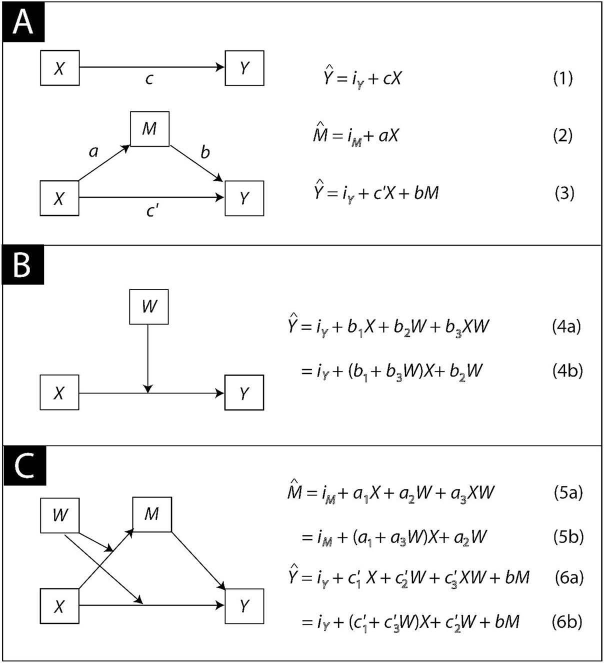
Figure 1. Simple Mediation (A), Simple Moderation (B), and a Conditional Process Model (C)
Total, Direct, and Indirect Effects
When M and Y are continuous variables, the mediation model in Figure 1, Panel A, typically is estimated using OLS regression or structural equation modeling software. Equations 1–3 in Figure 1, Panel A, repeated below, represent the models of Y and M in mathematical form, with the carets (^) representing estimated values. For simplicity in notation, we have excluded the residuals or “errors of estimation” from these equations.
 $$ \hat{Y}\hskip2pt =\hskip2pt {i}_Y+ cX $$
 $$ \hat{M}\hskip2pt =\hskip2pt {i}_M+ aX $$
 $$ \hat{Y}\hskip2pt =\hskip2pt {i}_Y+{c}^{\prime }X+ bM $$
The regression weight for X in Equation 1, Path c, is the total effect of X and quantifies the estimated difference in Y between two people (assuming people are the unit of analysis in the investigation you are conducting) that differ by one unit in X. When X is dichotomous and the two groups are represented in the data with two numbers that differ by one unit (a convention we recommend following, such 0 and 1 or –0.5 and 0.5), c is the difference observed between the means of Y in the two groups. The sign of c (and indeed, all of the paths in the model) is arbitrary and influenced by decisions about scaling of X and Y (or, when X is dichotomous, which group received the numerically larger value of X). That is, the sign of c is determined by whether higher on the construct X or Y measures or codes corresponds to higher or lower measurements of X or Y in the data.
There is a still widespread but mistaken belief—evidenced in the text of some published articles but also likely resulting in many other interesting studies with important findings languishing unpublished in file drawers—that a mediation analysis should only be performed when this total effect of X, path c, is statistically different from zero. According to this belief, if you cannot convincingly establish that X and Y are associated to a statistically significant degree, then you have not established that there is an effect of X to be mediated and so there is no point in estimating a mediation model. This view, made popular probably by an influential article by Baron and Kenny (Reference Baron and Kenny1986) that guided researchers for decades, contradicts what is now the conventional wisdom of methodologists and represented most concisely by Bollen (Reference Bollen1989) when he said “a lack of correlation does not disprove causation” (p. 52, italics present in the original). Though evidence of a statistically significant effect of X on Y often motivates questions about mediation in the first place, it is now widely understood and advocated among experts who think and write about mediation analysis for a living that this is neither a requirement for mediation analysis to be undertaken nor for mediation to be in operation in the process generating one’s data. O’Rourke & MacKinnon (Reference O’Rourke and MacKinnon2018) provide one of the better recent discussions of this perspective as well as some explanations, but there are others (e.g., Hayes, Reference Hayes2009; Reference Hayes2022; Kenny & Judd, Reference Kenny and Judd2014; Shrout & Bolger, Reference Shrout and Bolger2002).
The path analysis discussion that follows will help clarify this counterintuitive perspective. In a simple mediation model, X exerts is effect on Y through two additive pathways of influence. One of these pathways, and the one we care most about in a mediation analysis, is the indirect effect of X and is quantified as the product of path a, the regression coefficient for X in Equation 2, and path b, the regression coefficient for M in Equation 3. Path a estimates the difference in M between two people that differ by one unit on X, and path b estimates the difference in Y between two people that differ by one unit on M but who are equal on X. Multiplying them together results in ab, the estimated difference in Y attributable to a one unit difference in X that operates through the joint effect of X on M which in turn affects Y. When X is dichotomous, this can be interpreted as the part of the difference in Y between groups resulting from the mediation process captured by ab.
The sign of the indirect effect, ab, can be interpreted like a regression coefficient even though it is in reality a product of regression coefficients. A positive indirect effect means the mediation process at work results in those relatively higher in X estimated as relatively higher on Y, and a negative indirect effect means those relatively higher in X are estimated as relatively lower on Y. But substantively, the interpretation of the sign requires an examination of the signs of the components, a and b. The indirect effect will be positive if both a and b are positive or both are negative, whereas a negative indirect effect occurs if a or b are opposite in sign, irrespective of which is negative and which is positive. So don’t pop the champagne cork just because, for example, you predicted a positive indirect effect and that is what you found. If your theoretical rationale predicted a positive a and b path given the measurement scaling you used and therefore a positive indirect effect, but in your results a and b are both negative, then clearly you can’t claim support for your prediction and you need to go back to the theoretical drawing board.
The second pathway of influence is the direct effect of X, quantified as the regression coefficient for X, c’, in Equation 3. It estimates the difference in Y between two people that differ by one unit in X (or between the two groups on average if X is dichotomous and the groups are coded with two values that differ by one unit) that exists independent of differences between those people in M, or, rephrased, independent of the mediation process captured by the indirect effect. So whereas ab is the quantitative instantiation of the mediation process and what we care most about when conducting a mediation analysis, c’ is everything else. It is everything but the mechanism at work captured by the indirect effect.
These two pathways of influence, the indirect and direct effects of X, sum to produce the total effect of X: c = c’ + ab. This will always be true when using OLS regression to estimate Equations 1–3, so long as the same data are used to estimate the coefficients in each equation (and, if covariates are included, they are all included in each of the equations). Given that the total effect is the sum of two effects that may have different signs, it is easy to see how ab could be large even though c is small. And if ab and c’ are the same size but different in sign, c = 0. These scenarios do happen. There are many examples in the literature. So for this reason, among others, you should not insist that the total effect of X is statistically different from zero prior to conducting a mediation analysis.
Another important takeaway from this path analysis algebra is that the indirect effect of X is the difference between the total effect of X and the direct effect of X. That is ab = c – c’. So it is sensible to ask when conducting a mediation analysis what happens to the effect of X when M is controlled (Equation 3) relative to when M is left free to vary (Equation 1). The change in the effect of X with and without control for M is the indirect effect. That is what we care about. But what does not matter are the outcomes of hypothesis tests for c and c’. Whether c and/or c’ is statistically significant or their pattern (e.g., c statistically significant but c’ nonsignificant) tells us nothing about mediation.Footnote 2
Inference about the Indirect Effect
So the outcome of an inferential test of neither the total effect of X (path c) nor the direct effect of X (c’) tells us anything when our hypothesis is about mediation. The size of ab is not determined by c, c’, or their statistical significance or lackthereof. Statistical inference about mediation in the modern era focuses on inference about the product of a and b. It is the difference between the total and direct effects of X. We want to know whether zero can be plausibly discounted as a value of the indirect effect.
Until the last decade or so, researchers relied on joint hypothesis tests about a and b combined with a test of c in order to support an inference about mediation. That is, if a, b, and c are all statistically significant, then M can be deemed a mediator of the effect of X on Y so long as c’ is closer to zero than c. The inference about the indirect effect, using this approach, is merely a logical rather than a statistical one. That is, if we can claim both a and b are different from zero by some kind of inferential standard, then their product must be different from zero too and so no test of the product is needed. But this logic, outlined by Baron and Kenny (Reference Baron and Kenny1986) in their popular discussion of “criteria to establish mediation,” has fallen out of favor, though its use can still be found in articles published in TSJP (e.g., Caro-Cañizares, et al., Reference Caro-Cañizares, Díaz de Neira-Hernando, Pfang, Baca-Garcia and Carballo2018; Virkes et al., Reference Virkes, Seršić and Lopez-Zafra2017). The regression equations Baron and Kenny (Reference Baron and Kenny1986) described are still very important and are in fact the same equations in Figure 1 that we have relied on in this discussion. What has changed is the reliance on tests of significance for the components of the indirect effect. As discussed earlier, the signs of a and b certainly matter because their signs provide the substantive interpretation of their product. But whether both a and b are different from zero (sometimes called the test of joint significance) does not. What matters is whether the product of a and b is different from zero, since it quantifies how much X “moves” Y by “moving” M. There have been a few recent attempts to resurrect the moribund test of joint significance (e.g., Yzerbyt et al., Reference Yzerbyt, Muller, Batailler and Judd2018). We recommend letting it rest in peace and focusing your inference on ab irrespective of the outcome of hypothesis tests for a and b. For a more detailed discussion of this point, see Hayes (Reference Hayes2022).
But how do you conduct an inference about the product of regression coefficients? This topic was addressed in Baron and Kenny (Reference Baron and Kenny1986) and may account for why the Sobel test became a popular secondary approach to inference. The Sobel test (Sobel, Reference Sobel1982) is conducted by calculating the ratio of the point estimate to its standard error. A p-value for this test statistic, under the null hypothesis of no indirect effect, is derived from the standard normal distribution. Alternatively, a 95% confidence interval for the indirect effect can be constructed as approximately ab plus or minus two standard errors.
Like Baron and Kenny’s “criteria to establish mediation” and the test of joint significance, the Sobel test (also called the normal theory approach by some) has been criticized (e.g., Hayes, Reference Hayes2009) on the grounds of its performance and that it assumes the sampling distribution of ab is normal in form. However, the sampling distribution of the product of two regression coefficients typically is not normal. Rather, its shape is irregular in form and dependent on the population values of a and b. So the normal distribution is an inappropriate reference distribution for deriving p-values and confidence intervals. Furthermore, the Sobel test results in a test of mediation that is lower in power than alternatives and generates confidence intervals with coverage (i.e., containing the true value of the indirect effect) that does not correspond to the desired level of confidence. Nevertheless, researchers are still using it, including some who have published in TSJP (Virkes et al., Reference Virkes, Seršić and Lopez-Zafra2017). We recommend editors and reviewers who witness this practice nudge researchers toward modern and accepted alternatives to inference about the indirect effect.
What are these alternatives? There are several, including Monte Carlo confidence intervals (Preacher & Selig, Reference Preacher and Selig2012) and Bayesian methods (Yuan & MacKinnon, Reference Yuan and MacKinnon2009) but we recommend the percentile bootstrap confidence interval, as it has become the new standard and is easy to calculate with popular statistical software while making no assumptions whatsoever about the shape of the sampling distribution of the indirect effect. The mechanics of bootstrapping as applied to mediation analysis is discussed in detail elsewhere (Hayes, Reference Hayes2022; MacKinnon, Reference MacKinnon2008; Shrout & Bolger, Reference Shrout and Bolger2002). Below we provide only a brief overview.
To construct a bootstrap confidence interval, a new data set containing just as many cases as the original sample is constructed by sampling cases in the original data with replacement. In this bootstrap sample, the analysis is conducted and the indirect effect, called a bootstrap estimate of the indirect effect, is recorded. This process is repeated many times, preferably at least 1,000, through more is better. Once completed, the 2.5th and the 97.5th percentiles of this distribution of many bootstrap estimates serve as the lower and upper bounds on a 95% bootstrap confidence interval for the indirect effect. If zero is outside of the confidence interval, this provides statistical support for mediation. By contrast, if zero is between the endpoints of the confidence interval, then zero cannot be definitively ruled out as a plausible value of the indirect effect and one cannot claim support for mediation. Tweaking this method with some additional computation and statistical theory generates bias-corrected or bias-corrected and accelerated confidence intervals (Efron, Reference Efron1987), but these extra computations don’t particularly improve the test and can actually worsen the performance of the bootstrap method in some circumstances (Fritz et al., Reference Fritz, Taylor and MacKinnon2012; Hayes & Scharkow, Reference Hayes and Scharkow2013). Though bootstrapping is not always possible or can be difficult to construct for some kinds of research designs (e.g., multilevel designs, designs with complex sampling plans), our perspective is that when it can be conducted, it should be and when you do, it’s the only inferential test you need to report.
Illustration Using PROCESS
Bootstrapping is a computer-intensive method, but that doesn’t mean it is labor-intensive for you. Indeed, modern mediation analysis is perhaps simpler to undertake now with software you are already using than it ever has been. Although there are many choices available, we illustrate a mediation analysis using the PROCESS procedure described and documented in Hayes (Reference Hayes2022). It is freely available for SPSS, SAS, and RFootnote 3, widely-used in many disciplines, and it doesn’t take more than a few minutes to learn how to use it. In workshops we have taught over the years, we have found that a roomful of researchers can be successfully taught how to generate their first PROCESS output with little more than 10 minutes or so of training.
We use the data from our working example to estimate the total, direct, and indirect effects of similarity to the immigrant protagonist in the vignette (X, coded 0 for those in the dissimilar condition and 1 for those in the similar condition) on positive feelings toward immigrants (Y), with the indirect effect operating through identification with the immigrant (M). For this analysis we ignore the narrative voice manipulation. In the data, X, M, and Y are named similar, ident, and feeling, respectively. Only a single line of PROCESS code estimates the model and does the bootstrapping. In SPSS, SAS, and R, that line of code is
SPSS: process y=feeling/x=similar/m=ident/model=4/total=1/seed=34421.
SAS: %process (data=narratives,y=feeling,x=similar,m=ident,model=4,total=1,seed=34421)
R: process (data=narratives,y="feeling",x="similar",m="ident",model=4,total=1, seed=34421)
The resulting PROCESS output can be found in Appendix 1. The output contains three OLS regression analyses corresponding to Equations 1–3 in Figure 1, and the summary section at the bottom provides the direct, indirect, and total effects of similarity. Participants who read the vignette describing an immigrant similar to the typical Spaniard reported c = 1.771 units more positive feelings about immigrants, on average, than those who read about a dissimilar immigrant. This total effect is not statistically significant, but remember that c conveys nothing about mediation, and statistical significance of the total effect is not a requirement of mediation nor a prerequisite to conducting a mediation analysis.
This total effect of 1.771 units partitions into direct and indirect pathways of influence. The indirect effect is the product of the effect of similarity on identification and the effect of identification on positive feelings. As can be seen, those exposed to the similar immigrant identified with the immigrant by a = 0.112 units more on average relative to those exposed to the dissimilar immigrant. And the more a participant identified with the immigrant, the more positive the evaluation of immigrants (b = 9.566). Only the latter effect is statistically significant, but joint significance of the components of the indirect effect is not a requirement of mediation. It is the indirect effect that matters, which in this example is ab = 0.112(9.566) = 1.071, or 1.071 units of more positive feelings about immigrants, on average, resulting from the increase in identification resulting from similarity which, in turn, is associated with more positive feelings. However, observe that a bootstrap confidence interval for the indirect effect, based on 5,000 bootstrap samples (the default in PROCESS), includes zero (95% CI [–0.790, 3.006]). Thus, the results of this study do not support mediation of the effect of similarity on feelings toward immigrants by identification.
The direct effect is the difference between the groups in their feelings toward immigrants that results through some process other than identification. As can be seen, adjusting for differences between people in their identification, exposure to the dissimilar immigrant was associated with, on average, c’ = 0.700 more positive feelings about immigrants, though this is not statistically significant. Notice that, as promised, the total effect of X is the sum of the direct and indirect effects of X: c = c’ + ab = 1.771 = 0.700 + 1.071.
Although it would seem that this quest for evidence of mediation is a failure, in that it doesn’t reveal evidence consistent with mediation, we will see that to stop the analysis here would be a mistake, as similarity does seem to affect how participants feel about immigrants after exposure to the vignette. But this effect and the process at works depend on something we have not incorporated into this analysis.
Moderation Analysis
Whereas mediation analysis focuses on analyzing how an effect operates, moderation analysis is used when interest is directed toward questions about when that effect operates. Under which circumstances, or for which type of people, does X influence Y. In other words, when does affect X affect Y and when does it not, or when does X affect Y strongly versus weakly, or positively versus negatively? For example, in this journal, Correia et al. (Reference Correia, Salvado and Alves2016) observed that belief in a just world (X) was associated with helping behavior (Y) but only among people who showed higher self-efficacy to promote justice in the world. In this case, the perception of self-efficacy (W) acted as a moderator of the effect of belief in a just world on helping. Moderator variables represent those circumstances or situations that influence the size of X’s effect (Hayes, Reference Hayes2022). Also known as statistical interaction, moderation is of great relevance in research, as the introduction of a moderating variable into a theoretical explanation can deepen our understanding of the relationship between one variable and another (Holbert & Park, Reference Holbert and Park2020).
Most researchers are first introduced to the concept of moderation when learning about interaction in a factorial analysis of variance, the 2 × 2 factorial ANOVA being the simplest form. When two dichotomous variables are crossed in a 2 × 2 design, analysis of variance is typically used to estimate the main effect of each factor as well as their interaction, with the interaction capturing the extent to which the effect of one factor differs across values of the other factor. Evidence of interaction is typically then complemented by an analysis of simple effects, to test the effect of one factor at each of the levels of the other factor, thereby determining the conditions under which the effect of the first factor occurs, with the second factor playing the role of moderator.
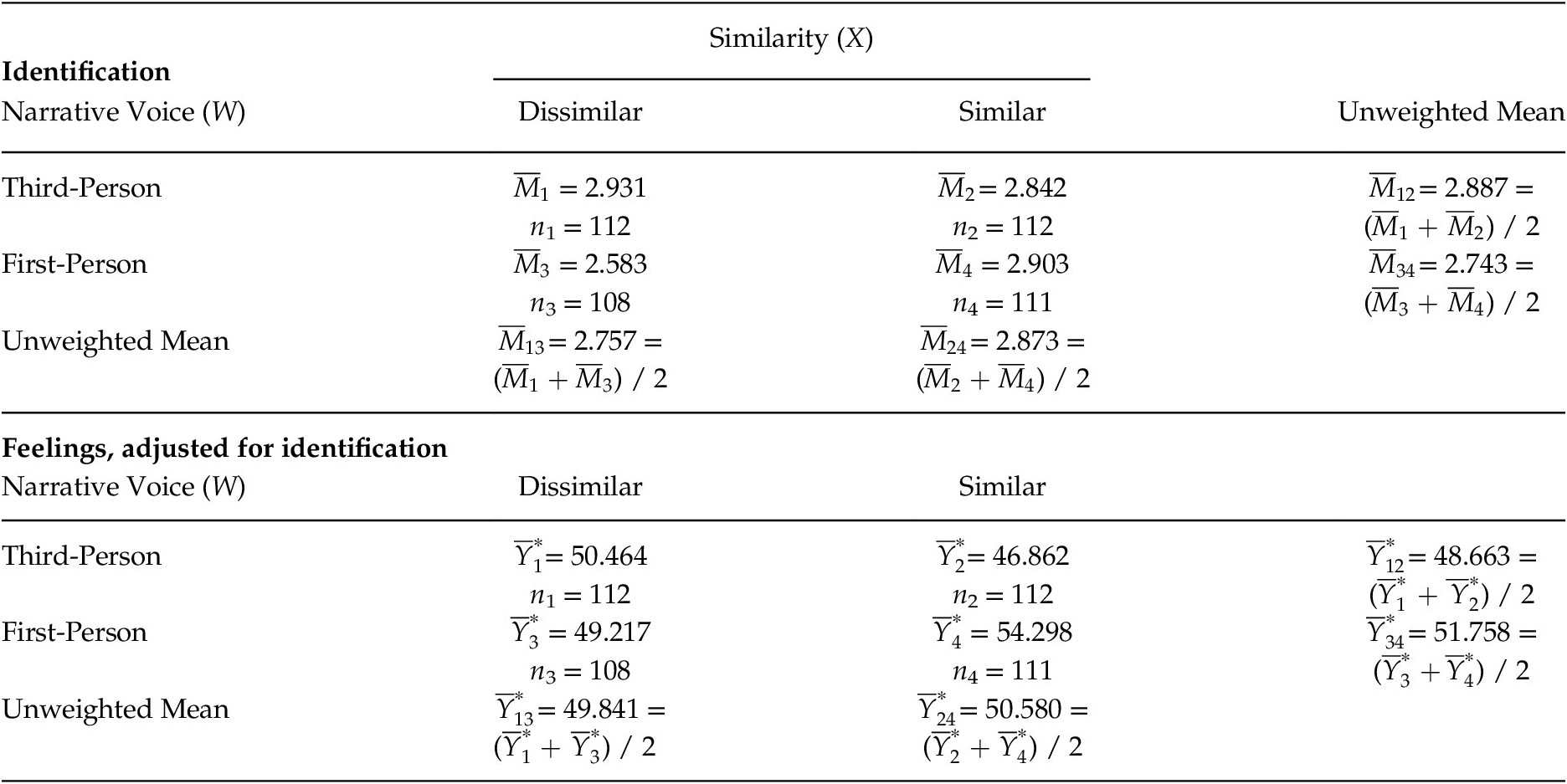
Recall from the section on mediation analysis that there was no statistically significant difference between the similar and dissimilar conditions (X) in feelings toward immigrants (Y). This was the total effect of X. A 2 × 2 ANOVA reveals, however, that the effect of similarity on feelings differed depends on whether the vignette is voiced in first- or third-person perspective. Table 1 provides the cell means in each of the four conditions, the unweighted marginal means and the F-ratios for the main and interaction effects.Footnote
4 The main effect of similarity, quantified as the difference between the unweighted column means,
 $ {\overline{Y}}_{24} $
–
$ {\overline{Y}}_{24} $
–
 $ {\overline{Y}}_{13} $
= 51.108 – 49.277 = 1.831, is not statistically significant, F(1, 439) = 0.558, p = .455. Nor is the main effect of voice statistically significant, F(1, 439) = 0.505, p = .478, quantified as the difference between the unweighted row means,
$ {\overline{Y}}_{13} $
= 51.108 – 49.277 = 1.831, is not statistically significant, F(1, 439) = 0.558, p = .455. Nor is the main effect of voice statistically significant, F(1, 439) = 0.505, p = .478, quantified as the difference between the unweighted row means,
 $ {\overline{Y}}_{34} $
–
$ {\overline{Y}}_{34} $
–
 $ {\overline{Y}}_{12} $
= 51.063 – 49.321 = 1.742. However, the interaction between similarity and voice is statistically significant, F(1, 439) = 6.563, p = .011. That is, the effect of similarity on feelings depends on (i.e., is moderated by) narrative voice. This interaction is quantified using the cell means as the difference between the simple effect of similarity in the first-person condition (
$ {\overline{Y}}_{12} $
= 51.063 – 49.321 = 1.742. However, the interaction between similarity and voice is statistically significant, F(1, 439) = 6.563, p = .011. That is, the effect of similarity on feelings depends on (i.e., is moderated by) narrative voice. This interaction is quantified using the cell means as the difference between the simple effect of similarity in the first-person condition (
 $ {\overline{Y}}_4 $
–
$ {\overline{Y}}_4 $
–
 $ {\overline{Y}}_3 $
= 55.117 – 47.009 = 8.108) and the simple effect of similarity in the third-person condition (
$ {\overline{Y}}_3 $
= 55.117 – 47.009 = 8.108) and the simple effect of similarity in the third-person condition (
 $ {\overline{Y}}_2 $
–
$ {\overline{Y}}_2 $
–
 $ {\overline{Y}}_1 $
= 47.098 – 51.545 = –4.447). That is, we can say that 8.108 and –4.447 are statistically different from each other. Rephrased, (
$ {\overline{Y}}_1 $
= 47.098 – 51.545 = –4.447). That is, we can say that 8.108 and –4.447 are statistically different from each other. Rephrased, (
 $ {\overline{Y}}_4 $
–
$ {\overline{Y}}_4 $
–
 $ {\overline{Y}}_3 $
) – (
$ {\overline{Y}}_3 $
) – (
 $ {\overline{Y}}_2 $
–
$ {\overline{Y}}_2 $
–
 $ {\overline{Y}}_1 $
) = 8.108 – (–4.447) = 12.555, is statistically different from zero.
$ {\overline{Y}}_1 $
) = 8.108 – (–4.447) = 12.555, is statistically different from zero.
Table 1. Mean Feeling toward Immigrants (Higher = More Positive) as a Function of Similarity and Narrative Voice Conditions

Note. Main effect of Similarity (X): 51.108 – 49.277 = 1.831, F(1, 439) = 0.558, p = .455. Main effect of Voice (W): 51.063 – 49.321 = 1.742, F(1, 439) = 0.505, p = .478. Interaction: (55.117 – 47.009) – (47.098 – 51.545) = 12.555, F(1, 439) = 6.563, p = .011.
Knowing from the test of interaction that these differences are significantly different from each other, significant interaction in 2 × 2 ANOVA is typically followed up by a simple effects analysis, conducting a statistical test for two of the simple effects at each of the two levels of the moderator. In this case, immigrants were perceived more positively after exposure to the similar immigrant relative to the dissimilar immigrant when the vignette was voiced from a first-person perspective,
 $ {\overline{Y}}_4 $
–
$ {\overline{Y}}_4 $
–
 $ {\overline{Y}}_3 $
= 55.117 – 47.009 = 8.108, F(1, 439) = 5.413, p = .020, but there was no statistically significant difference in feelings between the similar and dissimilar immigrant when voiced from a third-person perspective,
$ {\overline{Y}}_3 $
= 55.117 – 47.009 = 8.108, F(1, 439) = 5.413, p = .020, but there was no statistically significant difference in feelings between the similar and dissimilar immigrant when voiced from a third-person perspective,
 $ {\overline{Y}}_2 $
–
$ {\overline{Y}}_2 $
–
 $ {\overline{Y}}_1 $
= 47.098 – 51.545 = –4.447, F(1, 439)=1.666, p = .198.
$ {\overline{Y}}_1 $
= 47.098 – 51.545 = –4.447, F(1, 439)=1.666, p = .198.
A 2 × 2 ANOVA can be conducted using regression analysis, which is ultimately much more general and versatile because a regression approach does not require that the two variables being crossed be categorical. They can be categorical, continuous, or any combination of categorical and continuous. Furthermore, approaching the analysis from a regression perspective makes it simpler to integrate moderation with mediation analysis, which we do later. In the rest of this section, we describe how a regression model can be specified to express variable X’s effect on an outcome variable to be a function of a moderator W and how a 2 × 2 factorial analysis of variance can be replicated with a regression program. We also show how PROCESS simplifies the analysis and generates most everything needed for interpretation in one simple command line and output. For a more general discussion of moderation in regression analysis beyond case of a dichotomous X and W, see Aiken and West (Reference Aiken and West1991), Hayes (Reference Hayes2022), and Jaccard and Turrisi (Reference Jaccard and Turrisi2003).
A Variable’s Effect as a Function of a Moderator
Figure 1, Panel B, is a conceptual representation of a simple moderation model with a single moderating variable W modifying the relationship between X and Y. Assuming X and W are either dichotomous or continuous and the outcome variable Y is a continuous dimension suitable for analysis with OLS regression, this model is often estimated by regressing Y on X, W, and their product, as in Equation 4a in Figure 1, Panel B and below.
 $$ \hat{Y}\hskip2pt =\hskip2pt {i}_Y+{b}_1X+{b}_2W+{b}_3 XW $$
A mathematically equivalent form of this model is
 $$ \hat{Y}\hskip2pt =\hskip2pt {i}_Y+\left({b}_1+{b}_3W\right)X+{b}_2W\hskip2pt =\hskip2pt {i}_Y+{\theta}_{X\to Y}X+{b}_2W $$
where
 $ {\theta}_{X\to Y} $
= b
1 + b
3W. In this representation, it is apparent that in the moderated multiple regression model, the weight for X is not a single number but, rather, a function of W. That function is b
1 + b
3W. The output this function generates is sometimes called the simple slope of X, though we prefer the term conditional effect of X to make it explicit that it is the effect of X on the outcome variable conditioned on the moderator W being set to a specific value. Our use of
$ {\theta}_{X\to Y} $
= b
1 + b
3W. In this representation, it is apparent that in the moderated multiple regression model, the weight for X is not a single number but, rather, a function of W. That function is b
1 + b
3W. The output this function generates is sometimes called the simple slope of X, though we prefer the term conditional effect of X to make it explicit that it is the effect of X on the outcome variable conditioned on the moderator W being set to a specific value. Our use of
 $ {\theta}_{X\to Y} $
to the refer to the conditional effect of X on Y is consistent with Hayes (Reference Hayes2022). As will be seen, in the special case of two dichotomous variables X and W,
$ {\theta}_{X\to Y} $
to the refer to the conditional effect of X on Y is consistent with Hayes (Reference Hayes2022). As will be seen, in the special case of two dichotomous variables X and W,
 $ {\theta}_{X\to Y} $
= b
1 + b
3W quantifies either the main effect of X, one of the two simple effect of Xs, or nothing at all, depending on how the two groups defined by X and W are coded in the data.
$ {\theta}_{X\to Y} $
= b
1 + b
3W quantifies either the main effect of X, one of the two simple effect of Xs, or nothing at all, depending on how the two groups defined by X and W are coded in the data.
In Equations 4a and 4b, b
1 is the conditional effect of X on Y when W = 0. More specifically, b
1 is the estimated difference in Y between two cases in the data that differ by one unit in X but have a value of 0 for W. This is apparent by recognizing that
 $ {\theta}_{X\to Y} $
is a function of W which reduces to b
1 when W = 0. Similarly, b
2 is the conditional effect of W on Y when X = 0. This is seen most easily when Equation 4a is represented in another mathematically equivalent form, Ŷ = iY + (b
2 + b
3X)W + b
1X, where b
2 + b
3X is the conditional effect of W, which is a function of X. When X = 0, the conditional effect of W reduces to b
2.
$ {\theta}_{X\to Y} $
is a function of W which reduces to b
1 when W = 0. Similarly, b
2 is the conditional effect of W on Y when X = 0. This is seen most easily when Equation 4a is represented in another mathematically equivalent form, Ŷ = iY + (b
2 + b
3X)W + b
1X, where b
2 + b
3X is the conditional effect of W, which is a function of X. When X = 0, the conditional effect of W reduces to b
2.
In a moderation analysis, the coefficients b 1 and b 2 may or may not have a substantive interpretation, depending on how X and W are coded or, in the case of dichotomous X and W, what two numbers are used to represent the groups in the data. It is never correct to interpret b 1 as the effect of X on Y “controlling for” the effect of W and XW, and it usually is not correct to interpret b 1 as the “average effect” of X or the “main effect” of X, a term from analysis of variance that applies only when X and W are categorical but doesn’t generalize to all regression models. However, b 1 can be the main effect of X from a 2 × 2 ANOVA if X and W are coded appropriately, as will be seen. Similar arguments apply to the interpretation of b 2.
The regression weight for the product of X and W in Equations 4a and 4b, b
3, quantifies the difference in the effect of X as the moderator W changes by one unit. Recall from Equation 4b that the effect of X on Y (the estimated difference in Y between two cases that differ by one unit on X) is
 $ {\theta}_{X\to Y} $
= b
1 + b
3W. So when W = 0, X’s effect = b
1, when W = 1, X’s effect = b
1 + b
3, when W = 2, X’s effect is b
1 + 2b
3, and so forth. A statistically significant coefficient b
3 supports the claim that the effect of X on Y depends on the value of W and, therefore, that W moderates X’s effect. This interpretation does not require that X or W be dichotomous. It generalizes to any combination of continuous and dichotomous X and W. Modifications are needed to the regression model when X or W is multicategorical. For guidance in that situation, see Hayes (Reference Hayes2022) and Hayes and Montoya (Reference Hayes and Montoya2017).
$ {\theta}_{X\to Y} $
= b
1 + b
3W. So when W = 0, X’s effect = b
1, when W = 1, X’s effect = b
1 + b
3, when W = 2, X’s effect is b
1 + 2b
3, and so forth. A statistically significant coefficient b
3 supports the claim that the effect of X on Y depends on the value of W and, therefore, that W moderates X’s effect. This interpretation does not require that X or W be dichotomous. It generalizes to any combination of continuous and dichotomous X and W. Modifications are needed to the regression model when X or W is multicategorical. For guidance in that situation, see Hayes (Reference Hayes2022) and Hayes and Montoya (Reference Hayes and Montoya2017).
With evidence of moderation, common practice is to then probe that moderation by estimating and conducting a statistical test of the the conditional effect of X at various values of W. Called an analysis of simple slopes, the pick-a-point approach, or a spotlight analysis (Spiller et al., Reference Spiller, Fitzsimons, Lynch and McClelland2013), when W is dichotomous, the effect of X is tested for the two groups defined by W. When W is continuous, conventions often lead researchers to condition the estimates of X’s effect at arbitrary values of W that define “low,” “moderate,” and “high” in the distribution. A standard deviation below the mean, the mean, and a standard deviation of the mean is common. But Hayes (Reference Hayes2022) recommends using the 16th, 50th, and 84th percentiles, as they are more sensible representative values when the moderator is skewed but also corresponded to ± 1 standard deviation from the mean and the mean when W is exactly normally distributed. Rather than relying on arbitrary values of W, many advocate using the Johnson-Neyman technique (Bauer & Curran, Reference Bauer and Curran2005; Hayes & Matthes, Reference Hayes and Matthes2009), also called a floodlight analysis (Spiller et al., Reference Spiller, Fitzsimons, Lynch and McClelland2013), which analytically derives the values of W in which the conditional effect of X transitions between statistically significant and not. This results in the identification of regions of significance of X’s effect in the distribution of W.
Illustration Using PROCESS
PROCESS can conduct a moderation analysis in one simple command line with everything needed for interpretation in one tidy output. It generates estimates of the regression coefficients, a table of estimated values of the outcome for visualizing and interpreting the results, and it provides various options for probing an interaction, including the pick-a-point and Johnson Neyman techniques. We illustrate the use of PROCESS applied to this 2 × 2 design, with similarity as X, narrative voice as moderator W, and feelings toward immigrants as the outcome Y. Importantly, we conduct the analysis twice, one using a main effects parameterization which exactly replicates a 2 × 2 factorial analysis of variance and another which, though mathematically equivalent, produces estimates of b 1 and b 2 that have a different interpretation.
In the data as described thus far, the similarity (X) and voice (W) conditions are coded using 0 and 1. To replicate a 2
 $ \times $
2 factorial analysis of variance, we modify these codes, setting all values of 0 to –0.5 (X: Dissimilar condition; W: Third-person voice condition) and all values of 1 to 0.5 (X: Similar condition, W: First-person voice condition). These are stored in the data file with variable names similar2 and voice2. The PROCESS command below estimates the model
$ \times $
2 factorial analysis of variance, we modify these codes, setting all values of 0 to –0.5 (X: Dissimilar condition; W: Third-person voice condition) and all values of 1 to 0.5 (X: Similar condition, W: First-person voice condition). These are stored in the data file with variable names similar2 and voice2. The PROCESS command below estimates the model
SPSS: process y=feeling/x=similar2/w=voice2/model=1/plot=2.
SAS: %process (data=narratives,y=feeling,x=similar2,w=voice2,model=1,plot=2)
R: process (data=narratives,y="feeling",x="similar2",w="voice2",model=1,plot=2)
The PROCESS output can be found in Appendix 2, and the regression coefficients and conditional effects are found in Table 2. This is called a main effects parameterization because the use of –0.5 and 0.5 for X and W produces estimates of b
1 and b
2 that correspond to the main effects of X and W from a 2 × 2 ANOVA. Notice that b
1 = 1.831, which is the main effect for X (similarity). It is the difference between the column means in Table 1 (
 $ {\overline{Y}}_{24} $
–
$ {\overline{Y}}_{24} $
–
 $ {\overline{Y}}_{13} $
= 51.108 – 49.277 = 1.831). And its p-value is .455, which is the same as the p-value for the F-ratio for the main effect in the ANOVA. These are mathematically equivalent tests. Indeed, the F-ratio from the ANOVA used to produce the p-value is equal to the square of the t value for b
1 in the regression analysis (see Appendix 2).
$ {\overline{Y}}_{13} $
= 51.108 – 49.277 = 1.831). And its p-value is .455, which is the same as the p-value for the F-ratio for the main effect in the ANOVA. These are mathematically equivalent tests. Indeed, the F-ratio from the ANOVA used to produce the p-value is equal to the square of the t value for b
1 in the regression analysis (see Appendix 2).
Table 2. Moderation Analysis of a 2 × 2 Design Using a Main Effects (–0.5/0.5 Coding) and a Simple Effects (0/1 coding) Parameterization. The Outcome is Feelings toward Immigrants
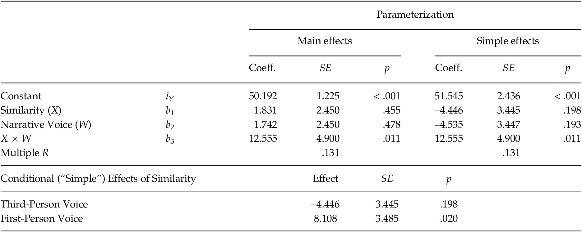
Likewise, when using a main effects parameterization, b
2 = 1.742 is the main effect of narrative voice (W) from the ANOVA. Observe that b
2 corresponds to the difference between the row means in Table 1:
 $ {\overline{Y}}_{34} $
–
$ {\overline{Y}}_{34} $
–
 $ {\overline{Y}}_{12} $
= 51.063 – 49.321 = 1.742. The p-value of .478 for b
2 in the regression is the same as the p-value for the F-ratio from the ANOVA, and F from the ANOVA is t
2 for b
2 from the regression. These are mathematically identical tests.
$ {\overline{Y}}_{12} $
= 51.063 – 49.321 = 1.742. The p-value of .478 for b
2 in the regression is the same as the p-value for the F-ratio from the ANOVA, and F from the ANOVA is t
2 for b
2 from the regression. These are mathematically identical tests.
As in the 2 × 2 ANOVA reported in Table 1, the regression weight for the product of X and W, b
3, in the regression model is statistically significant, with the same p-value of .011 as the p-value for the F-ratio from the ANOVA. And F from the ANOVA = t
2 for b
3 from the regression analysis. And observe that the value of b
3 of 12.555 is equal to the difference between the simple effects of similarity across the two voice conditions. That is, b
3 = (
 $ {\overline{Y}}_4 $
–
$ {\overline{Y}}_4 $
–
 $ {\overline{Y}}_3 $
) – (
$ {\overline{Y}}_3 $
) – (
 $ {\overline{Y}}_2 $
–
$ {\overline{Y}}_2 $
–
 $ {\overline{Y}}_1 $
) = 8.108 – (–4.447).
$ {\overline{Y}}_1 $
) = 8.108 – (–4.447).
In addition to producing the main and interaction effects from the ANOVA, PROCESS also generates the two conditional or simple effects of similarity in the section labelled “Conditional effects of the focal predictor at values of the moderator.” These come from the function
 $ {\theta}_{X\to Y} $
= b
1 + b
3W = 1.831 + 12.555W. Plugging W = –0.5 (for the third-person voice condition) into this function yields –4.446, which is equivalent to the simple effect
$ {\theta}_{X\to Y} $
= b
1 + b
3W = 1.831 + 12.555W. Plugging W = –0.5 (for the third-person voice condition) into this function yields –4.446, which is equivalent to the simple effect
 $ {\overline{Y}}_2 $
–
$ {\overline{Y}}_2 $
–
 $ {\overline{Y}}_1 $
in Table 1. The p-value is .198, just as from earlier in our discussion of the 2 × 2 ANOVA introducing this section. Repeating for the first-person voice condition, plugging W = 0.5, into this function generates 8.108, which is equivalent to the simple effect
$ {\overline{Y}}_1 $
in Table 1. The p-value is .198, just as from earlier in our discussion of the 2 × 2 ANOVA introducing this section. Repeating for the first-person voice condition, plugging W = 0.5, into this function generates 8.108, which is equivalent to the simple effect
 $ {\overline{Y}}_4 $
–
$ {\overline{Y}}_4 $
–
 $ {\overline{Y}}_3 $
in Table 1. The p-value is .020, just as it was when probing the interaction in the 2 × 2 ANOVA.
$ {\overline{Y}}_3 $
in Table 1. The p-value is .020, just as it was when probing the interaction in the 2 × 2 ANOVA.
The plot option in PROCESS, when toggled on with option 2 as in the command above, generates a table of estimated values of Y from the regression model in the four conditions formed by crossing X and W. These can be found under the heading “Data for visualizing the effect of the focal predictor” in the PROCESS output. As can be seen in Appendix 2, these four values correspond to the cell means in Table 1. Standard errors and confidence intervals for these cell means are also provided in the PROCESS output.
Earlier we said that b 1 and b 2 are rarely interpreted as “main effects” are in a factorial analysis of variance. In this example, they do have this interpretation but only because of our use of –0.5 and 0.5 for the coding of X and W. Had we used different numbers for X and W to code the groups, b 1 and b 2 would not have this interpretation, but the model would otherwise be identical in that it would have the same R, fit the data equally well, generate the same estimates of Y for the four conditions, and the test of interaction would be the same, as would the test of simple or conditional effects.
We illustrate by running this analysis again but this time using 0 and 1 for the coding of X and W. Appendix 3 contains the resulting PROCESS output (using the variables named similar and voice in the data and the PROCESS command above for X and W, respectively), and the model is summarized in Table 2. The use of 0 and 1 for X and W produces the simple effects parameterization of the model, so called because b 1 and b 2 now represent two of the four simple effects in the 2 × 2 table of means in Table 1 rather than the main effects of X and W. Other than the regression constant, the only differences between the models and the two PROCESS outputs are the weights for b 1 and b 2 along with their standard errors, t- and p-values, and confidence intervals. The test of interaction is the same, as are the conditional effects of X, the fit of the model, and the estimated values of Y the model generates for the four groups.
Remember that in Equations 4a and 4b, the interpretation of regression coefficient for X is the effect of X when W = 0 and the coefficient for W is the effect of W when X = 0. In this example, that means that b
1 = –4.446 is the simple effect of the similarity manipulation (X) among those assigned to the third-person condition, because for people in that condition, W is set to 0 in the data. In Table 1, this corresponds to
 $ {\overline{Y}}_2 $
–
$ {\overline{Y}}_2 $
–
 $ {\overline{Y}}_1 $
= 47.098 – 51.545. These two means are not statistically different from each other, p = .198. And b
2 = –4.535 and the corresponds to the simple effect of the narrative voice manipulation among those assigned to the dissimilar condition (because for those in the low similarity condition, X = 0 in the data). In Table 1, this corresponds to
$ {\overline{Y}}_1 $
= 47.098 – 51.545. These two means are not statistically different from each other, p = .198. And b
2 = –4.535 and the corresponds to the simple effect of the narrative voice manipulation among those assigned to the dissimilar condition (because for those in the low similarity condition, X = 0 in the data). In Table 1, this corresponds to
 $ {\overline{Y}}_3 $
–
$ {\overline{Y}}_3 $
–
 $ {\overline{Y}}_1 $
= 47.009 – 51.545. These two means are not statistically different from each other, p = .193.
$ {\overline{Y}}_1 $
= 47.009 – 51.545. These two means are not statistically different from each other, p = .193.
The moral is that regression analysis can be used to analyze the popular 2 × 2 design and PROCESS makes this easy, but the weights for X and W in the model will only correspond to the main effects from a factorial analysis of variance if you code X and W appropriately to produce the main effects parameterization. In most any other coding system, b 1 and b 2 are not the main effects of X as the term is used in analysis of variance.
Integrating Moderation and Mediation: Conditional Process Analysis
Conditional processes analysis is the analytical integration of mediation and moderation analysis. It is used when an investigator hypothesizes or theorizes that the mechanism by which one variable influences another through one or more mediators is dependent on the size or value of one or more moderator variables. Whereas mediation analysis focuses on how an effect operates and moderation analysis reveals when that effect exists or is large versus small, conditional process analysis is used to answer questions about the “when of the how.” Under what circumstances, or for what kinds of people (“when”), is a particular mechanism (“how”) at work and when is it not, or when is the size or strength of that mechanism large versus small. A defining feature of a conditional process model is that such a model allows an indirect effect (typically), a direct effect (sometimes), or both to depend on at least one moderator.
Conditional process analysis is a fairly new term, introduced into the methodology literature in the first edition of Hayes (Reference Hayes2022) published in 2013. But the idea of integrating mediation and moderation analysis, as well as various approaches to doing so, dates back further than 2013 (see, e.g., Baron & Kenny, Reference Baron and Kenny1986; Edwards & Lambert, Reference Edwards and Lambert2007; Fairchild & MacKinnon, Reference Fairchild and MacKinnon2009; Morgan-Lopez & MacKinnon, Reference Morgan-Lopez and MacKinnon2006; Muller et al., Reference Muller, Judd and Yzerbyt2005; Preacher et al., Reference Preacher, Rucker and Hayes2007) primarily using easily-confused terms such as the analysis of “moderated mediation” or “mediated moderation.” And there are now many examples of conditional process analysis in the psychological literature (Gabbiadini et al., Reference Gabbiadini, Riva, Andrighetto, Volpato and Bushman2016; Igartua et al., Reference Igartua, Wojcieszak and Kim2019; Knoster & Goodboy, Reference Knoster and Goodboy2020; Muralidharan & Kim, Reference Muralidharan and Kim2020), though we found only a few instances in our perusal of some recent volumes of TSJP. Álvaro et al. (Reference Álvaro, Garrido, Pereira, Torres and Barros2019), for example, considered the moderating role of gender when analyzing the indirect effect of unemployment on depression through the reduction of self-esteem, observing that “unemployment is associated with lower self-esteem, which predicts higher symptoms of depression, but this relationship can only be observed in men, and not in women” (p. 7). In that study, unemployment was X, self-esteem was the mediator M, depression was the outcome of interest Y, and the gender of the respondents played a moderating role in their model.
A conditional process model can take a dizzying number of forms. Just a small sampling of the possibilities with only a single mediator can be found in Figure 2. In Panel A is a first stage conditional process model, so-named because it specifies a moderator (W) of the indirect effect of X in the first stage of the mediation process (i.e., the effect of X on M). Figure 2, Panel B, is a second stage conditional process model, with moderator W specified as moderating the second stage of the mediation process (i.e., the effect of M on Y). This form of a second-stage model also allows for moderation of the direct effect by W. The model in Panel C is a blend of the first and second stage conditional process models in Panels A and B, with a single moderator modifying all three of the paths of a simple mediation model. Another form of the first and second stage conditional process model is found in Panel D, which differs from the others in that it has two moderators, with W moderating the first stage and Z moderating the second stage of the indirect effect. Considering that a mediation model can have several mediators in either parallel or serial form, and with one or more of the paths of an indirect effect moderated by the same or different variables, the number of possible conditional process models is practically endless.
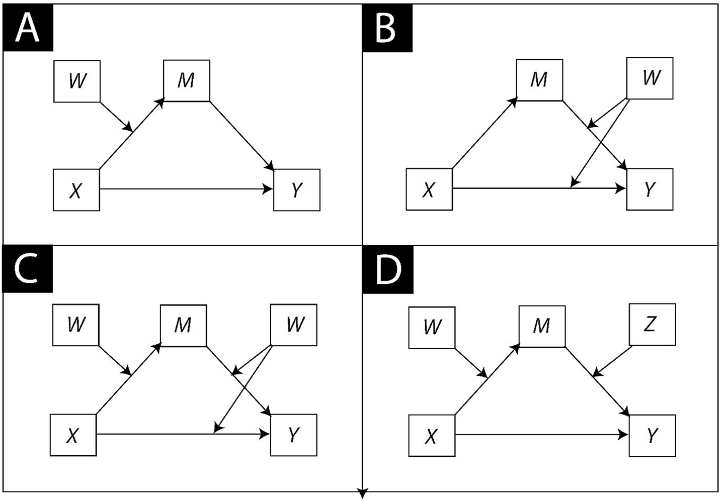
Figure 2. Examples of Some of the Many Possible Conditional Process Models
A simple and tempting but highly problematic approach to conditional process analysis to avoid but nevertheless still found in the literature is to split the sample into subgroups or strata, such as males and females (e.g., Carvalho & Hopko, Reference Carvalho and Hopko2011), or older and younger people (e.g., Grøntved et al., Reference Grøntved, Steene-Johannessen, Kynde, Franks, Helge, Froberg, Anderssen and Andersen2011), or in experimental and control conditions, and then conducting a mediation analysis in each group. Evidence of moderation of the mechanism is reported when the indirect effect seems larger in one group than in another or is statistically significant in one group but not the other. Adding insult to injury is the construction of the strata by artificially categorizing people in the sample (e.g., into “low” and “high” groups) using a mean or median split of a continuous variable being used as the moderator. This strategy has all the problems of subgroups conditional process analysis discussed in Hayes (Reference Hayes2022; e.g., no formal test of the difference between indirect effects, differential power for tests when the statra differ in size, among other problems), while also adding all of the problems associated with artificial categorization of continuous variables (see e.g., Rucker et al., Reference Rucker, McShane and Preacher2015). A properly conducted conditional process analysis can be done with a continuous moderator just as easily as it can with a categorical moderator, so there is never any need to artificially categorize a moderator prior to analysis.
Example and Illustration Using PROCESS
Unlike in the sections on mediation and moderation, we will not discuss conditional process analysis in generic form, because the mathematics of a conditional process model are highly dependent on the form the model takes, of which there are many as already discussed (for a discussion of various models and how they are set up in the form of a set of regression equations, see e.g., Edwards & Lambert, Reference Edwards and Lambert2007; Hayes, Reference Hayes2022; Preacher et al., Reference Preacher, Rucker and Hayes2007). Instead, we will move right to a concrete example based on the same study we have used to this point. In the context of that example we will talk about the specifics of the modeling math as a way of illustrating some general principles.
Conditional process analysis is implemented in the PROCESS macro and takes most of the programming and computational burdens off you. It has many conditional process models preprogrammed, and you can create a custom model with up to 6 mediators and two moderators by using the procedure discussed in Appendix B of Hayes (Reference Hayes2022). Although an SEM program could be used, this would require manually programming the mathematics of the model and many lines of code to visualize and probe components of the model and construct various tests of interest. Although there are some advantages to using an SEM program, with observed (as opposed to latent variables) variables PROCESS generally produce the same results while requiring far less effort and programming expertise (Hayes et al., Reference Hayes, Montoya and Rockwood2017; Hayes & Rockwood, Reference Hayes and Rockwood2020).
In this illustration, we estimate the model in Figure 1, Panel C, with the similarity manipulation as X, identification with the immigrant as mediator M, feelings toward immigrants as Y, and narrative voice as moderator W. This is a first stage conditional process model that allows for moderation of the direct effect as well as the indirect effect. The moderation of the indirect effect was expected to operate by narrative voice influencing the effect of similarity on identification with the immigrant. With no basis for believing that the influence of identification on feelings toward immigrants would differ between the narrative voice conditions, this effect was not specified as moderated. The moderation of the direct effect follows from our finding that, without considering the mediator, similarity differentially influenced feelings toward immigrants depending on narrative voice, as we reported in the moderation section.
In practice, researchers should think carefully about what form of conditional process model is appropriate given the existing literature and theorizing on the phenomenon they are studying. As discussed above, many models can be constructed from a set of mediator(s) and moderator(s). Exploratory conditional process analysis is certainly possible, especially with a tool like PROCESS that makes it easy to try different models, but doing so runs the risk of overfitting the data. Without a strong theoretical rational that leads you to choose a particular model, we recommend always attempting to replicate a finding based on exploration before attempting to publish.
This conditional process model is preprogrammed in PROCESS as model number 8. It is specified by two regression equations, one for M and one for Y:
 $$ \hat{M}\hskip2pt =\hskip2pt {i}_M+{a}_1X+{a}_2W+{a}_3 XW $$
which is equivalent to
 $$ \hat{M}\hskip2pt =\hskip2pt {i}_M+\left({a}_1+{a}_3W\right)X+{a}_2W\hskip2pt =\hskip2pt {i}_M+{\theta}_{X\to M}X+{a}_2W $$
where
 $ {\theta}_{X\to M} $
= a
1 + a
3W is the conditional effect of X on M, and
$ {\theta}_{X\to M} $
= a
1 + a
3W is the conditional effect of X on M, and
 $$ \hat{Y}\hskip2pt =\hskip2pt {i}_Y+{c}_1^{\prime }X+{c}_2^{\prime }W+{c}_3^{\prime } XW+ bM $$
which is equivalent to
 $$ \hat{Y}\hskip2pt =\hskip2pt {i}_Y+\left({c}_1^{\prime }+{c}_3^{\prime }W\right)X+ bM\hskip2pt =\hskip2pt {i}_Y+{\theta}_{X\to Y}X+ bM $$
where
 $ {\theta}_{X\to Y}\hskip2pt =\hskip2pt {c}_1^{\prime }+{c}_3^{\prime }W $
, the conditional direct effect of X on Y. The indirect effect of X on Y through M is the product of the effect of X on M and the effect of M on Y, as always. But in this model, the effect of X on M is a function of W. Nevertheless, multiplying these two effects together gives
$ {\theta}_{X\to Y}\hskip2pt =\hskip2pt {c}_1^{\prime }+{c}_3^{\prime }W $
, the conditional direct effect of X on Y. The indirect effect of X on Y through M is the product of the effect of X on M and the effect of M on Y, as always. But in this model, the effect of X on M is a function of W. Nevertheless, multiplying these two effects together gives
 $$ {\theta}_{X\to M}b\hskip2pt =\hskip2pt \left({a}_1+{a}_3W\right)b\hskip2pt =\hskip2pt {a}_1b+{a}_3 bW $$
as the conditional indirect effect of X on Y. It is conditional because it is a function of W, a linear function. Its value will depend on the value of W inserted into Equation 7 after estimation of the model coefficients, as well as the value of
 $ {a}_3b $
, which is the index of moderated mediation.
$ {a}_3b $
, which is the index of moderated mediation.
Only a single line of PROCESS code, below, is required. In this example, we stick with the main effects parameterization of the 2 × 2 design by using similar2 and voice2 as X and W in the command line, as in our discussion of moderation. The choice of the main effects parameterization in this example has no effect on the estimates of the (conditional) direct and indirect effects or the test of moderated mediation discussed below. Had we used similar and voice in the command, the results would be identical, although a few of the regression coefficients estimated using Equations 5 and 6 would change, for the reasons described in the section above on moderation.
SPSS: process y=feeling/x=similar2/m=ident/w=voice2/model=8/plot=2/seed=34421.
SAS: %process (data=narratives,y=feeling,x=similar2,m=ident,w=voice2,model=8,plot=2, seed=34421)
R: process (data=narratives,y="feeling",x="similar2",m="ident",w=”voice2”,model=8,plot=2,seed=34421)
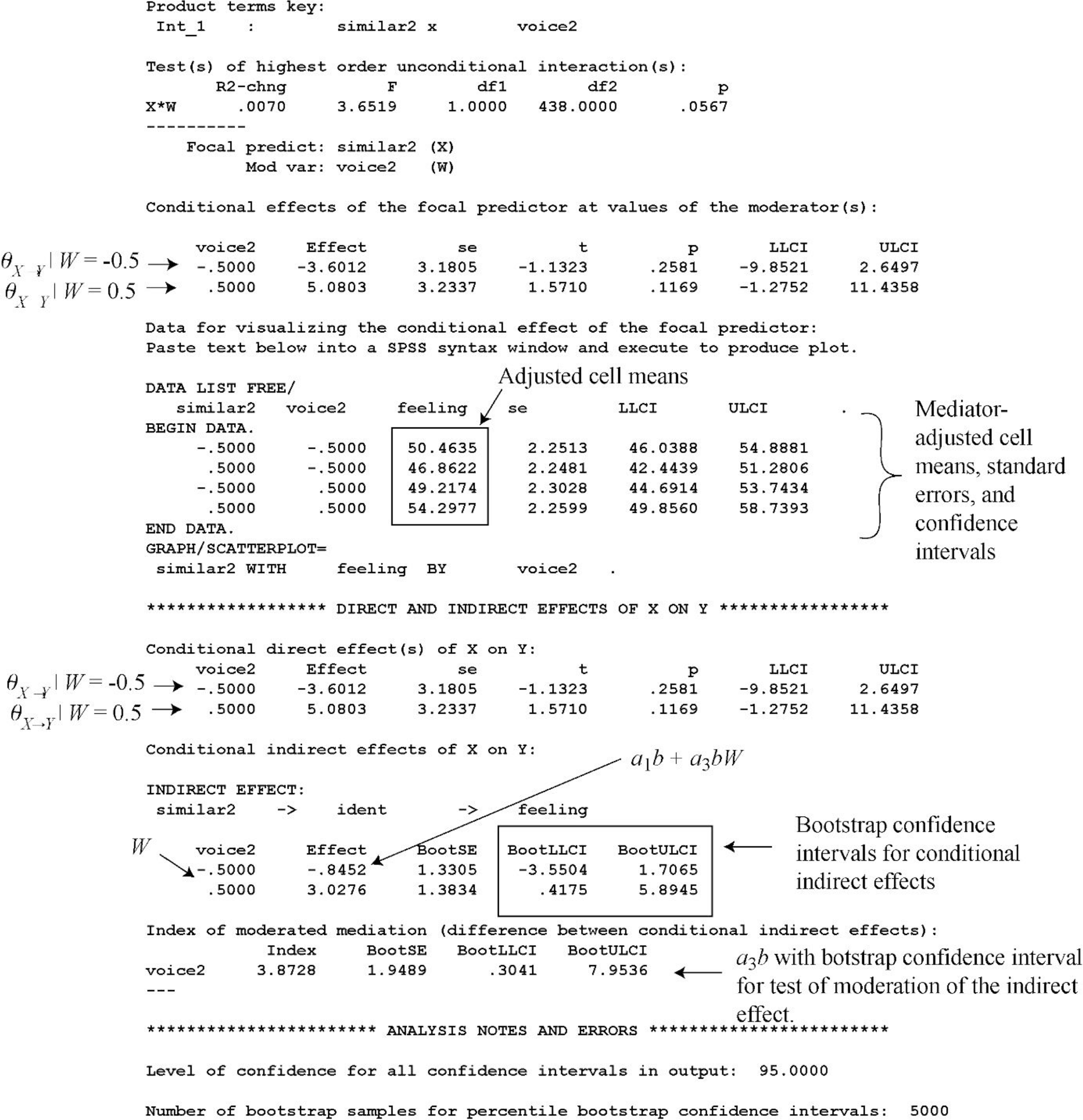
The resulting output can be found in Appendix 4, and a summary of the regression coefficients, conditional effects, and the test of moderated mediation is found in Table 3. The first section of output is the first stage component of the conditional process model, which in this example is equivalent to a 2 × 2 factorial ANOVA with identification as the outcome variable, since we are using a main effects parameterization. This is the model of identification represented by Equations 5a and 5b. Recall from the mediation analysis earlier in this paper that there was no statistically significant association between similarity and identification. Yet we see here that in fact, the effect of similarity on identification depends on narrative voice, as evidenced by the significant interaction in this part of the model, a
3 = 0.409, p = .042. The cell means are found in the PROCESS output below the regression model as well as in Table 4. As discussed in the moderation section, the regression coefficient of 0.409 for the product is the difference between the two conditional (“simple”) effects of similarity in the two narrative voice conditions. That is, a
3 = (
 $ {\overline{M}}_4 $
–
$ {\overline{M}}_4 $
–
 $ {\overline{M}}_3 $
) –
$ {\overline{M}}_3 $
) –
 $ \Big({\overline{M}}_2 $
–
$ \Big({\overline{M}}_2 $
–
 $ {\overline{M}}_1 $
) = (2.903 – 2.583) – (2.842 – 2.931) = 0.409.
$ {\overline{M}}_1 $
) = (2.903 – 2.583) – (2.842 – 2.931) = 0.409.
Table 3. Conditional Process Analysis of a 2 × 2 Design using a Main Effects (–0.5/0.5 coding) Parameterization, First Stage Moderated Mediation with Moderation of the Direct Effect

Table 4. Mean Identification with the Immigrant and Mediator-Adjusted Feelings toward Immigrants as a Function of Similarity and Narrative Voice
The conditional or simple effects of similarity on identification can be found in the PROCESS output and are defined by the function
 $ {\theta}_{X\to M} $
= a
1 + a
3W = 0.115 + 0.409W. Plugging in W = –0.5 (third-person) and W = 0.5 (first-person) into this function generates the two estimates of the conditional effect of similarity on identification. In the third-person condition,
$ {\theta}_{X\to M} $
= a
1 + a
3W = 0.115 + 0.409W. Plugging in W = –0.5 (third-person) and W = 0.5 (first-person) into this function generates the two estimates of the conditional effect of similarity on identification. In the third-person condition,
 $ {\theta}_{X\to M} $
| (W = –0.5) = –0.089, meaning participants in the similar condition identified less (by 0.089 units on average) with the immigrant than did those in the dissimilar condition (
$ {\theta}_{X\to M} $
| (W = –0.5) = –0.089, meaning participants in the similar condition identified less (by 0.089 units on average) with the immigrant than did those in the dissimilar condition (
 $ {\overline{M}}_2 $
–
$ {\overline{M}}_2 $
–
 $ {\overline{M}}_1 $
= 2.842 – 2.931 = –0.089), though this difference is not statistically significant (p = .528). In the first-person condition,
$ {\overline{M}}_1 $
= 2.842 – 2.931 = –0.089), though this difference is not statistically significant (p = .528). In the first-person condition,
 $ {\theta}_{X\to M} $
| (W = 0.5) = 0.320, meaning participants in the similar condition identified more with the immigrant (by 0.320 units on average) than did those in the dissimilar condition (
$ {\theta}_{X\to M} $
| (W = 0.5) = 0.320, meaning participants in the similar condition identified more with the immigrant (by 0.320 units on average) than did those in the dissimilar condition (
 $ {\overline{M}}_4 $
–
$ {\overline{M}}_4 $
–
 $ {\overline{M}}_3 $
= 2.903 – 2.583 = 0.320). This difference is statistically significant, p = .026.Footnote
5
$ {\overline{M}}_3 $
= 2.903 – 2.583 = 0.320). This difference is statistically significant, p = .026.Footnote
5
The outcome of tests of significance for neither the interaction nor the conditional effects in this model are particularly pertinent, however, as we care about the indirect effect of similarity on feelings through identification and whether there is difference between the two conditions in this (conditional) indirect effect. To construct the test and estimate the indirect effect in the two conditions, we need to first obtain the effect of identification on feelings (M on Y), the second stage component of the process, estimated with b in Equations 6a and 6b. This is in the second part of the PROCESS output in the model of feeling toward immigrants. As can be seen, the regression coefficient for identification (M) is 9.467, p < .001. Those who identified more with the immigrant reported more positive feelings toward immigrants in general.
As with the first stage component, the statistical significance of the effect of identification on feelings is also not particularly pertinent, as it too is not the indirect effect. As discussed earlier, we multiply the conditional effect of similarity on identification,
 $ {\theta}_{X\to M} $
= a
1 + a
3W by the effect of identification on feelings, b, yielding the function (a
1 + a
3W)b = a
1b + a
3bW, or 1.091 + 3.873W in this analysis. Plugging W = –0.5 into this function generates –0.845 for the indirect effect in the third-person condition. Those in the similar condition who read a vignette written from third-person perspective identified less with the immigrant than did those in the dissimilar condition,
$ {\theta}_{X\to M} $
= a
1 + a
3W by the effect of identification on feelings, b, yielding the function (a
1 + a
3W)b = a
1b + a
3bW, or 1.091 + 3.873W in this analysis. Plugging W = –0.5 into this function generates –0.845 for the indirect effect in the third-person condition. Those in the similar condition who read a vignette written from third-person perspective identified less with the immigrant than did those in the dissimilar condition,
 $ {\theta}_{X\to M} $
| (W = –0.5) = –0.089, and less identification translated into less positive feelings about immigrants (b = 9.467). The product of these two effects is –0.089(9.467) = –0.845, the conditional indirect effect of similarity in the third-person condition. Plugging W = 0.5 into this function generates 3.028 for the indirect effect of similarity in the first-person condition. The similar narrative written in first-person perspective resulted in greater identification with the immigrant than did the dissimilar narrative,
$ {\theta}_{X\to M} $
| (W = –0.5) = –0.089, and less identification translated into less positive feelings about immigrants (b = 9.467). The product of these two effects is –0.089(9.467) = –0.845, the conditional indirect effect of similarity in the third-person condition. Plugging W = 0.5 into this function generates 3.028 for the indirect effect of similarity in the first-person condition. The similar narrative written in first-person perspective resulted in greater identification with the immigrant than did the dissimilar narrative,
 $ {\theta}_{X\to M} $
| (W = 0.5) = 0.320, which in turn translated into more positive feelings about immigrants (b = 9.467). The product of these two effects is 0.320(9.467) = 3.028, the conditional indirect effect of similarity in the first-person condition.
$ {\theta}_{X\to M} $
| (W = 0.5) = 0.320, which in turn translated into more positive feelings about immigrants (b = 9.467). The product of these two effects is 0.320(9.467) = 3.028, the conditional indirect effect of similarity in the first-person condition.
Both of these conditional indirect effects are found in the PROCESS output under the heading “Conditional indirect effects of X on Y” along with bootstrap confidence intervals for inference. As can be seen, the confidence interval for the conditional indirect effect in the third-person condition includes zero (95% CI [–3.550, 1.707]) whereas for the first-person condition, the confidence interval is entirely above zero (95% CI [0.418, 5.895]).
Although this is consistent with moderation of mediation (mediation in the first-person but not the third-person narrative condition), difference in significance does not mean significantly different. A formal test of moderated of mediation requires testing whether these conditional indirect effects differ from each other. The difference between them, 3.028 – (–0.845), is the index of moderated mediation, a 3b = 3.873, and the weight for W in the function defining the conditional indirect effect (Equation 7). Rather than an outdated piece-meal approach recommended by Muller et al. (Reference Muller, Judd and Yzerbyt2005) and still advocated by Yzerbyt et al. (Reference Yzerbyt, Muller, Batailler and Judd2018) that focuses on tests of significance for a 3 and b, Hayes (Reference Hayes2015) recommends a single inference for the index of moderated mediation as the simplest and most direct test of moderated mediation. The index of moderated mediation is the change in the indirect effect as W changes by one unit. In our case, our two narrative voice groups differ by one unit on W (–0.5 and 0.5) and so a 3b is the difference between the indirect effects in the two groups. From the PROCESS output, a bootstrap confidence interval for the index of moderation mediation is entirely positive (95% CI [0.304, 7.954]), meaning that the indirect effect of similarity on feelings through identification differs between the first and third-person narrative voice conditions. That is, mediation is moderated.
A conditional process model is a mediation model, and in a mediation model there are indirect and direct effects. We have shown that the indirect effect in this example is moderated, with evidence of mediation of the effect of similarity on feelings through identification in the first-person but not the third-person narrative voice condition. In this model, the direct effect of similarity is also specified as moderated by narrative voice. This is captured in Equations 6a and 6b, which is this example is the regression equivalent of a 2 × 2 factorial analysis of covariance (ANCOVA) with the mediator functioning as a covariate (remember that the direct effect of X in a mediation model is the effect of X on Y controlling for the mediator).
In a 2 × 2 design, interpretation of the analysis is based on the relative sizes of main or simple effects that are quantified as differences between cell means or functions of those means. In an ANCOVA, which the model of Y in this example is but in regression form, interpretation is based on differences between adjusted means. Adjusted means are estimates of what each group mean would be if groups were equal on the covariate(s). In this example, the adjusted means are the cell means adjusted for differences between the groups in the mediator. This is accomplished by generating estimates of the outcome variable from the regression model for each of the groups when the mediator is equal to the sample mean. Using the regression coefficients for the model of feelings in the PROCESS output, the model that produces these adjusted means is
 $$ {\overline{Y}}^{\ast}\hskip2pt =\hskip2pt 23.547+0.740X+3.095W+8.681 XW+9.467\left(\overline{M}\right) $$
where
 $ \overline{M} $
= 2.817, the sample mean identification with the immigrant in the vignette. These adjusted cell means can be found in the PROCESS output in the model for feelings, under the heading “Data for visualizing the conditional effect of the focal predictor.” They can also be found in Table 4. The discussion below is based on these adjusted means.
$ \overline{M} $
= 2.817, the sample mean identification with the immigrant in the vignette. These adjusted cell means can be found in the PROCESS output in the model for feelings, under the heading “Data for visualizing the conditional effect of the focal predictor.” They can also be found in Table 4. The discussion below is based on these adjusted means.
From Equation 6b, the direct effect of X,
 $ {\theta}_{X\to Y}, $
is defined by the function
$ {\theta}_{X\to Y}, $
is defined by the function
 $ {\theta}_{X\to Y}\hskip2pt =\hskip2pt {c}_1^{\prime }+{c}_3^{\prime }W $
= 0.740 + 8.681W. This function produces the conditional direct effects while
$ {\theta}_{X\to Y}\hskip2pt =\hskip2pt {c}_1^{\prime }+{c}_3^{\prime }W $
= 0.740 + 8.681W. This function produces the conditional direct effects while
 $ {c}_3^{\prime } $
, which is also the weight for the product of X and W in the regression model for Y, captures the change in the direct effect of X on Y as W changes by one unit. As can be seen in Appendix 4 and Table 3,
$ {c}_3^{\prime } $
, which is also the weight for the product of X and W in the regression model for Y, captures the change in the direct effect of X on Y as W changes by one unit. As can be seen in Appendix 4 and Table 3,
 $ {c}_3^{\prime } $
= 8.681, but this just misses statistical significance at the .05 level (p = .057). This weight for the product is the difference between the conditional direct effects in the two narrative voice groups. Using this function, in the third-person narrative condition (when W = –0.5), the conditional direct effect
$ {c}_3^{\prime } $
= 8.681, but this just misses statistical significance at the .05 level (p = .057). This weight for the product is the difference between the conditional direct effects in the two narrative voice groups. Using this function, in the third-person narrative condition (when W = –0.5), the conditional direct effect
 $ {\theta}_{X\to Y} $
| (W = –0.5) = –3.601 (equivalent to
$ {\theta}_{X\to Y} $
| (W = –0.5) = –3.601 (equivalent to
 $ {\overline{Y}}_2^{\ast }- $
 $ {\overline{Y}}_1^{\ast } $
in Table 4) and, from the PROCESS output, not statistically significant, p = .258. In the first-person narrative condition (when W = 0.5), the conditional direct effect is
$ {\overline{Y}}_1^{\ast } $
in Table 4) and, from the PROCESS output, not statistically significant, p = .258. In the first-person narrative condition (when W = 0.5), the conditional direct effect is
 $ {\theta}_{X\to Y} $
| (W = 0.5) = 5.080 (equivalent to
$ {\theta}_{X\to Y} $
| (W = 0.5) = 5.080 (equivalent to
 $ {\overline{Y}}_4^{\ast }- $
 $ {\overline{Y}}_3^{\ast } $
in Table 4) and also not statistically significant. Notice that
$ {\overline{Y}}_3^{\ast } $
in Table 4) and also not statistically significant. Notice that
 $ {c}_3^{\prime } $
is indeed equal to the difference between these conditional direct effects:
$ {c}_3^{\prime } $
is indeed equal to the difference between these conditional direct effects:
 $ {c}_3^{\prime } $
= (
$ {c}_3^{\prime } $
= (
 $ {\overline{Y}}_4^{\ast }- $
 $ {\overline{Y}}_3^{\ast}\left)-\right({\overline{Y}}_2^{\ast }- $
 $ {\overline{Y}}_1^{\ast}\Big) $
= 5.080 – (–3.601) = 8.681.Footnote
6
$ {\overline{Y}}_1^{\ast}\Big) $
= 5.080 – (–3.601) = 8.681.Footnote
6
Given that the evidence does not convincingly support moderation of the direct effect, this model could be simplified by estimating a model that fixes the direct effect to be a constant rather than a function of narrative voice. This can be done easily using PROCESS with Model 7, which eliminates W and XW from Equations 6a and 6b (all of the preprogrammed models available in PROCESS are documented in Appendix A of Hayes, Reference Hayes2022). We consider this an exercise for you to try. As you will see when conducting the analysis, substantively, the results of this study don’t change with this modification to the model. The indirect effect is still moderated by narrative voice, with evidence of mediation only in the first-person condition. And the direct effect is not statistically significant.
Conclusion
In this paper, we described the fundamentals of statistical mediation and moderation analysis and their integration as conditional process analysis in the popular 2 × 2 experimental design, though the principles generalize to other designs including designs with no experimental manipulation or continuous variables. We illustrated these techniques using nothing more complicated than OLS regression analysis implemented in the PROCESS macro for SPSS, SAS, and R. Our working example illustrates how an analysis that fails to explore the contingencies of a relationship (or lack thereof) can result in inaccurate conclusions. In the section on mediation analysis, we saw no statistically significant effect of the similarity of the protagonist in the vignette on identification with the immigrant or feelings about immigrants in general, and no evidence of mediation. Yet a moderation analysis showed that the similarity manipulation did in fact seem to influence people’s feelings about immigrants, but only when the immigrant’s story was told from a first-person perspective. Furthermore, contrary to the results from a simple mediation analysis, this effect of similarity seemed by driven by (i.e., mediated by) identification with the immigrant in the story, but not when it was framed from a third-person perspective. That is, this similarity-to-identification-to-feelings process seemed to be in operation with a first-person but not a third-person narrative.
Our focus in this paper has been on data analysis and showing how certain analytical techniques can be employed easily with the help of PROCESS when studying the contingencies and mechanisms of effects assumed to be causal. But statistical methods cannot by themselves establish cause–effect, which ultimately is problem of design and theoretical argumentation, not data analysis. Experimental designs and longitudinal designs are certainly better than correlational designs at establishing temporal precedence and ruling out certain alternative explanations for findings that abound in correlational studies. However, even tightly controlled experimental designs do not address certain ambiguities in interpretation of results from a mediation or conditional process analysis. For example, although the manipulation of X combined with random assignment affords causal interpretation of the effect of X on M and Y in a mediation and conditional process analysis; it says nothing about the direction of cause between M and Y or rule out alternative explanations (such as confounding) for that association. Various solutions to solving such problems are described in the methodology literature aimed at improving the design of such experiments (Spencer at al., Reference Spencer, Zanna and Fong2005; Pirlott & MacKinnon, Reference Pirlott and MacKinnon2016). It is always important to advance a cogent and convincing theoretical argument for why relationships you observe are or are likely to be causal in nature. Statistical methods are mathematical tools that enable us to discern order in the chaos of our data and detect signs of processes that can explain the relationship between variables. But causal inference is based more on design, theory, and argument, than it is on statistics. “Inferences are products of our mind and not our mathematics” (Hayes, Reference Hayes2022; Hayes & Rockwood, Reference Hayes and Rockwood2017, p. 54).
Appendices
Appendix 1: PROCESS Output from a Simple Mediation Analysis

Appendix 2: PROCESS Output from a Simple Moderation Analysis Replicating a 2 x 2 Factorial ANOVA (Main Effects Parameterization)
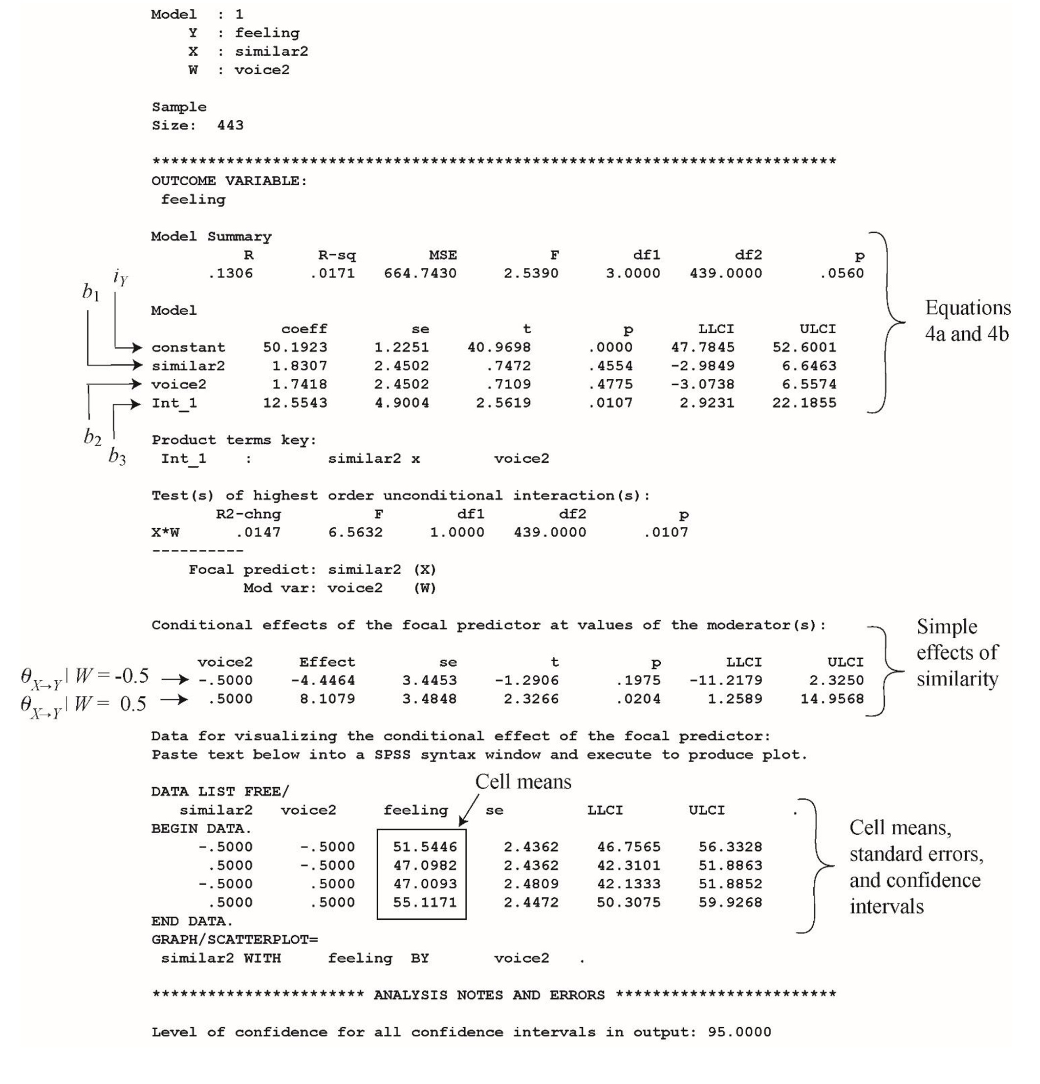
Appendix 3: PROCESS Output from a Simple Moderation Analysis of the 2 x 2 Design (Simple Effects Parameterization)

Appendix 4: PROCESS Output from a Conditional Process Analysis of the 2 x 2 Design (Main Effects Parameterization)