Introduction
In recent years, with the rapid development of the mobile Internet and popularization of the Internet of Things, the demands of communication services have grown explosively. Wireless sensor networks, as one of the core technologies of the Internet of Things, can be used in the fields of precision agriculture, logistics, smart grids, security, surveillance, habitat monitoring, health, etc. [Reference Kurt and Tavli1]. The path-loss model is an important theoretical basis for power control, link analysis, and tracking orientation in wireless sensor networks [Reference Xu, Zhang and Yang2].
Studies on the path-loss model mainly concentrate on model parameter estimation and specific environmental modeling. In general, the path-loss types are divided into indoor models and outdoor models [Reference Degli-Esposti, Vitucci and Martin3]. The indoor models include the International Telecommunications Union (ITU) model [Reference Rama Rao, Balachander, Nishesh and Prasad4, Reference Ata, Shahateet, Jawadeh and Amro5], chan model, attenuation factor model [Reference Seidel and Rappaport6, Reference Xu, Zhang, Gao, Zhang and Wu7], one-slope model [Reference Rappaport and McGillem8, Reference Ai, Cheffena and Li9], etc. The outdoor models include the Egli model [Reference Egli10, Reference Joshi, Dietrich, Anderson, Newhall, Davis, Isaacs and Barnett11], Okumura model [Reference Okumura, Ohmori, Kawano and Fukua12, Reference Katiyar and Mittal13], Hata model [Reference Hata14, Reference Daisy, Zheng and Magdy15], etc. In indoor rooms and corridors, there are a large number of walls; thus, the wireless signal transmission will result in reflections. Although the floor penetration loss factor is taken into account, the ITU model is not accurate enough because of neglecting the multipath effect. The chan model considers both the frequency factor and the distance factor; however, it does not consider the multipath and shadow effects. When low accuracy of indoor field strength prediction value is required, the chan model is a good choice. The attenuation factor model is very simple, and can only provide a very rough estimate of the indoor path-loss. The one-slope model is the general model that is used to compute the average path-loss without detailed knowledge of the surrounding environment. The one-slope model only takes into account the distance between the transmitting and receiving antennas. The one-slope model is applicable to free spaces or unimpeded spaces; however, its prediction error is large under complex indoor environmental conditions [Reference Wang, Song, Kong and Zhang16, Reference Hamzah, Baharudin, Shah, Zainal Abidin and Ubin17]. In this paper, a new indoor path-loss model is established considering matching coefficient, polarization matching factor, normalized field intensity direction function, and wall reflection effect.
The structure of this paper is as follows. In section “Theoretical derivation”, the theory of the Friis-extension (Friis-EXT) model is introduced. In section “Measurement”, the measurement method of the wireless channel is described. In section “Result”, the proposed method is compared with traditional methods, such as the ITU model, chan model, one-slope model, and the attenuation factor model. In section “Conclusion”, the conclusion is stated.
Theoretical derivation
In the indoor multipath environment, the antenna that receives the electromagnetic wave signal can be described as follows [Reference Ma18].
In Fig. 1(a), the antenna receives incident electromagnetic waves from different directions in space and transmits them to the load Z L. The area of the dotted line in Fig. 1(b) is the equivalent circuit of the receiving antenna, e R is the electromotive force excited by external electromagnetic waves on the antenna oscillator, Z A is the internal resistance of the electromotive force, and Z L is the load impedance of the receiving antenna.

Fig. 1. Receiving antenna and equivalent circuit. (a) Receiving antenna, and (b) equivalent circuit.
From the equivalent circuit of the receiving antenna, we can obtain the receiving power that is transferred from the receiving antenna to the load [Reference Ma18].
 $$P_R = \displaystyle{1 \over 2}\vert I \vert ^2R_L = \displaystyle{1 \over 2}\displaystyle{{e_R^2} \over {{\lpar {R_A + R_L} \rpar }^2 + \lpar {X_A + X_L} \rpar {}^2}}\cdot R_L.$$
In formula (1), R A and X A are the input resistance and reactance of the receiving antenna, respectively, and R L and X L are the load resistance and reactance, respectively.
When the load and receiving antenna are conjugate matched (Z L = Z A*), the load obtains the maximum output power, which is called the maximum receiving power P RM.
 $$P_{RM} = \displaystyle{{e_R^2} \over {8R_A}}.$$
The relationship between the receiving power and maximum receiving power is
 $$P_R = \tau P_{RM},$$
where τ is called the matching coefficient, which represents the matching degree of the load and receiving antenna.
 $$\tau = \displaystyle{{{\rm 4}R_AR_L} \over {{\lpar {R_A + R_L} \rpar }^2 + \lpar {X_A + X_L} \rpar {}^2}}.$$
When the load and receiving antenna are conjugate matched, τ = 1, otherwise τ < 1.
If the receiving antenna undergoes a loss, R A = R ΣA + R LA (R ΣA and R LA are the radiation resistance and loss resistance, respectively). Then, the maximum receiving power is
 $$P_{RM} = \displaystyle{{e_R^2} \over {8R_{\sum A}}} \cdot \displaystyle{{R_{\sum A}} \over {R_A}} = P_{Ropt}\eta _A,$$
where η A is the antenna efficiency, whose physical meaning is the ratio of radiation resistance to the total resistance of antenna, and P R opt = e R2/8R ΣA is the optimum receiving power.
According to the reciprocal theory [Reference Ma18],
 $$e_R = \overrightarrow E (\theta, \phi )\cdot \overrightarrow e l_eF(\theta, \phi ).$$
In formula (6),  $$\overrightarrow E $$ (θ, Φ) is an incident electric field,
  $$\overrightarrow e $$ is a unit vector of antenna oscillator direction, l e is the effective length of the receiving antenna, and F(θ, Φ) is the normalized field intensity direction function of the receiving antenna, where
 $$\overrightarrow E (\theta, \phi )\cdot \overrightarrow e = E\cos (\xi ).$$
In formula (7), E is the electric field strength value, ξ is the angle of the incoming wave electric field vector and receiving antenna oscillator. cos(ξ) is the polarization matching factor. Therefore, formula (6) can be expressed as
 $$e_R = El_eF(\theta, \phi )\cos (\xi ).$$
The physical meaning of formula (8) is that the induced electromotive force of the receiving antenna is equal to the product of the normalized field intensity direction function of the antenna and the projection of incoming wave electric field on the effective length of the antenna oscillator. Substituting formulas (8) and (5) into formula (3), P R can be written as
 $$P_R = \displaystyle{{E^2l_e^2 F^2(\theta, \phi )} \over {8R_{\sum A}}} \cdot \eta _A\cdot \tau \cdot \cos ^2(\xi ).$$
Using the relationship between the effective length and direction coefficient [Reference Song, Zhang and Huang19]: D = 30 k 2l e2/R ΣA, P R can be expressed by
 $$P_R = \displaystyle{{E^2F^2(\theta, \phi )} \over {240k^2}}\cdot D\cdot \eta _A\cdot \tau \cdot \cos ^2(\xi ),$$
where k is the wave number, which is equal to 2π/λ, λ is the wavelength of the transmitting electromagnetic wave. The power density p and the electric field strength have the relationship [Reference Song, Zhang and Huang19]:
 $$p = \displaystyle{{E^2} \over {240\pi}}. $$
At the distance of d from the transmitting antenna, p can also be expressed as the power of the unit sphere area with radius d.
 $$p = \displaystyle{{P_TG_T} \over {4\pi d^2}}.$$
In formula (12), P T is the transmitting power, G T is the gain of transmitting antenna, d is the distance to transmitting antenna.From formulas (11) and (12), it can be obtained as
 $$E^2 = \displaystyle{{60P_TG_T} \over {d^2}}.$$
By substituting formula (13) into (10), P R can be written by
 $$P_R = \displaystyle{{P_TG_T\lambda ^2F^2(\theta, \phi )} \over {{(4\pi d)}^2}}\cdot D\cdot \eta _A\cdot \tau \cdot \cos ^2(\xi ).$$
Generally, the antenna gain is equal to the antenna efficiency multiplied by the directional coefficient
 $$G_R = D\cdot \eta _A,$$
where G R is the gain of the receiving antenna, by substituting formula (15) into formula (14), the relationship between P R and G R can be obtained as
 $$P_R = \displaystyle{{P_TG_T\lambda ^2F^2(\theta, \phi )} \over {{(4\pi d)}^2}}\cdot G_R\cdot \tau \cdot \cos ^2(\xi ).$$
When the matching coefficient τ is equal to 1, the polarization matching factor cos(ξ) is equal to 1 and the normalized field intensity direction function F(θ, Φ) is equal to 1. Formula (16) can be expressed as
 $$P_R = \displaystyle{{P_TG_TG_R\lambda ^2} \over {{(4\pi d)}^2}}.$$
Formula (17) is the Friis formula [Reference Kurt and Tavli1], and thus, we call formula (16) as Friis-EXT method. Finally, the path-loss is
 $$PL = \displaystyle{{P_T} \over {P_R}} = \displaystyle{{{(4\pi d)}^2} \over {G_TG_R\lambda ^2\tau {\cos} ^2(\xi )F^2(\theta, \phi )}},$$
which is expressed in dB as
 $$\eqalign{ PL =& 10[\log ((4\pi d)^2)-\log (G_T)-\log (G_R)-\log (\lambda ^2) \cr & -\log (\tau )-\log (\cos ^2(\xi ))-\log (F^2(\theta, \phi ))].} $$
Measurement
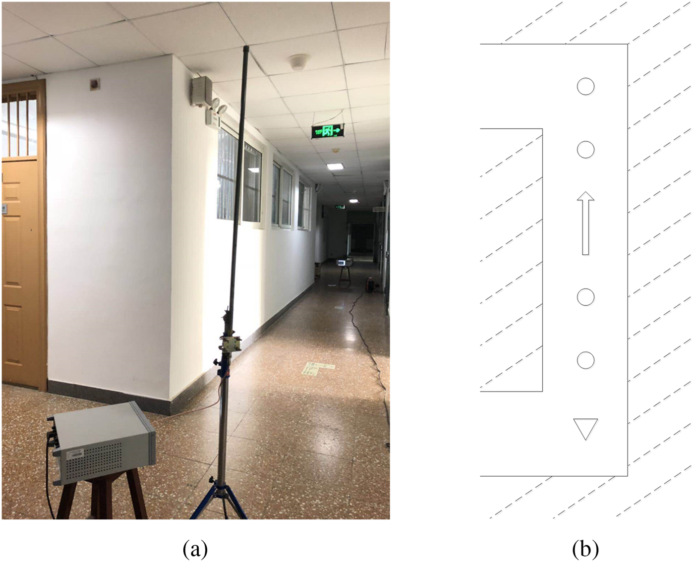
In this section, the indoor corridor environment is configured to conduct the measurement. The corridor is 35 m long and 3 m wide. The relative permittivity of the wall is equal to 6. The experiment scene is shown in Fig. 2(a). At the experiment site, one transmitting point and 10 receiving points are arranged to transmit and receive signals, respectively. The distance between every two adjacent points is 3 m, and the layout diagram is shown in Fig. 2(b), where the transmitting antenna is placed at the triangular point, which is 1 m above the ground. The receiving antenna is placed at the circular point, of which the height is set to 0.5 and 1 m, respectively. The radio frequency signal source AV1441A produced by Ceyear and a dipole antenna TQJ-2400AT10 produced by KenBoTong are chosen as the transmitting devices, and the spectrum analyzer N1996A produced by Keysight and a dipole antenna TQJ-2400E produced by KenBoTong are chosen as the receiving devices. The radiation patterns of transmitting and receiving antennas are shown in Fig. 3. The 2.4 GHz signal is generated by the signal source with a transmitting power of 0 dBm. In the experiment, the transmitting antenna maintains vertical polarization during measurement, and the receiving antenna is set at three angles opposite the transmitting antenna, which are 0, 30, and 60°, and while the receiving antenna measures three sets of data at each height. The measurement data are shown in Tables 1–3.
Table 1. 0° angle measurement data

Table 2. 30° angle measurement data

Table 3. 60° angle measurement data
Result
According to formula (19), the input parameters are set as follows. The transmitting power P T is set as 0 dBm, the transmitting antenna gain G T is 10 dBi, and the receiving antenna gain G R is 3 dBi. λ is the wavelength that corresponds to the 2.4 GHz electromagnetic wave, and the impedance parameters of the receiving antenna are R A = 38.92 Ω and X A = −3.64 Ω. The matching coefficient τ can be calculated according to formula (4). The normalized field intensity direction function F(θ, Φ) of the receiving antenna is equal to sin(θ). The polarization matching factor cos(ξ) can be configured by different angles. Additionally, the reflection factors are considered during the calculation. Since the field strength is weak along the axis direction of the antenna oscillator, the top and the bottom of reflective surfaces are ignored, and four reflective surfaces are considered (except the ceiling and ground). Subsequently, path-loss is obtained by superposing one direct wave and four reflected waves. The relative dielectric constant of cement is applied to calculate the reflectivity of the wall according to the formula (20):
 $$\gamma _\bot = \left( {\displaystyle{{\cos (\alpha )-\sqrt {{{{\varepsilon_2} / \varepsilon}}_1-{\sin}^2(\alpha )}} \over {\cos (\alpha ) + \sqrt {{{{\varepsilon_2} / \varepsilon}}_1-{\sin}^2(\alpha )}}}} \right)^2,$$
where α is the incident angle, ε 1 is the relative permittivity of air, which is equal to 1, and ε 2 is the relative permittivity of the wall, which is equal to 6. Formula (16) shows that the receiving power is inversely proportional to the square of the distance. The paths of the second and multiple reflections are relatively longer, and the reflectivity of the wall is calculated for each reflection, so we ignore the reflection power of the second and multiple reflections since their power is low enough to be negligible. After the electromagnetic wave is reflected by each wall, only one path can reach the receiving antenna. So the reflection point on each surface can be determined. Take one surface as an example, as shown in Fig. 4. The reflection angle is equal to the incident angle, and the test path is parallel to the corridor, so the calculation of the path distance of the reflected wave is
 $$l = 2\sqrt {{\left( {\displaystyle{d \over 2}} \right)}^2 + {\left( {\displaystyle{w \over 2}} \right)}^2}, $$
where l is the path distance of the reflected wave, w is the corridor wide, and d is the distance between the transmitting and receiving antennas.

Fig. 2. Measurement layout. (a) Experiment scene, and (b) layout diagram.
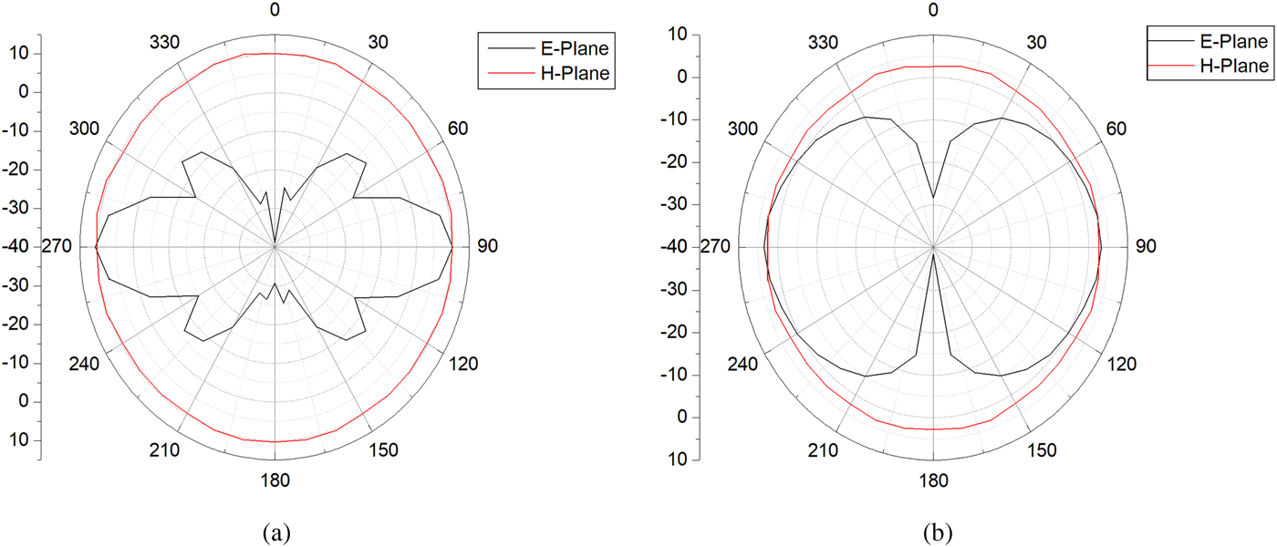
Fig. 3. Radiation patterns. (a) Transmitting antenna, and (b) receiving antenna.

Fig. 4. Reflection path.
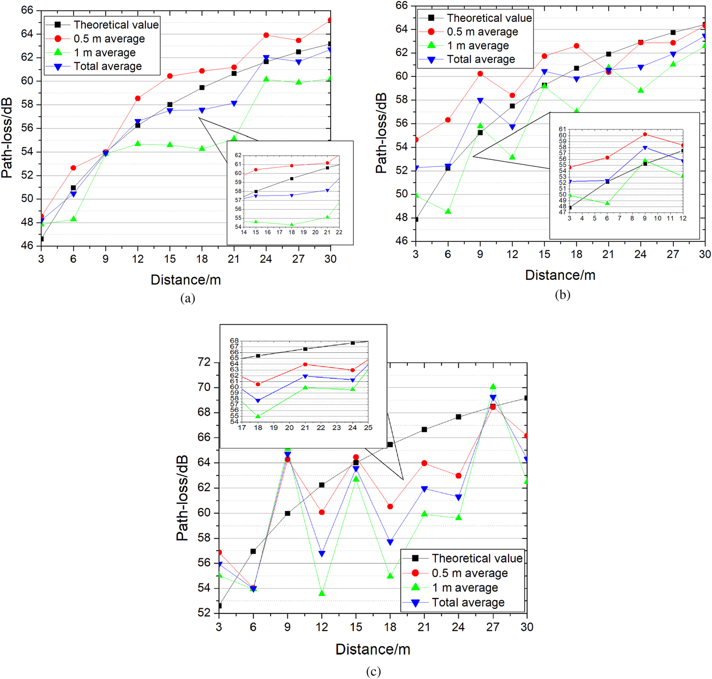
As shown in Fig. 5, the path-loss graph is obtained according to Friis-EXT method expressed in formula (19).

Fig. 5. Comparison of the theoretical and measured values at different polarization angles. (a) 0° polarization angle, (b) 30° polarization angle, and (c) 60° polarization angle.
For observation, the average of three sets of the measured data is calculated at each height, respectively, and the total average of six sets of the measured data of two heights is calculated too. Figure 5(a) shows the comparison of the measured value and the predicted value of 0° polarization angle. The maximum error of 0.5 m high of receiving antenna is 2.5 dB at 15 m, and the maximum error of 1 m high of receiving antenna is 5.5 dB at 21 m, and the maximum error between the total average and the predicted value is 2.5 dB at 21 m. Figure 5(b) shows the comparison of the measured value and the predicted value of 30° polarization angle. The maximum error of 0.5 m high of receiving antenna is 6.5 dB at 3 m, and the maximum error of 1 m high of receiving antenna is 4 dB at 12 m, and the maximum error between the total average and the predicted value is 4.5 dB at 3 m. Figure 5(c) shows the comparison of the measured value and the predicted value of 60° polarization angle. The maximum error of 0.5 m high of receiving antenna is 5 dB at 18 m, and the maximum error of 1 m high of receiving antenna is 10 dB at 18 m, and the maximum error between the total average and the predicted value is 7.5 dB at 18 m. Since the receiving antenna is artificially adjusted, the angle is not very accurate, resulting in a large deviation between the measured value of 60° and the theoretical value. In general, the theoretical values match the measured values closely. As is observed in Fig. 5, the path-loss is attenuated in accordance with the logarithmic law.
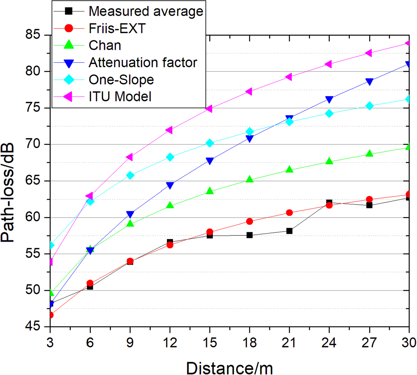
To validate the effectiveness of the proposed model, Friis-EXT method is compared with traditional methods, such as the ITU model, chan model, one-slope model, and the attenuation factor model. Since the traditional methods do not consider the polarization matching of the antennas, we use the 0° angle in the Friis-EXT model to compare with other methods. Due to the limited space, the height difference of the receiving antenna cannot be made too large, so the influence of the antenna height on the path-loss can be ignored. The average of six sets of measured data is taken for comparison. The results are shown in Fig. 6.

Fig. 6. Comparison of different models.
From Fig. 6, we observe that the differences between the traditional methods and measured data are very clear. The errors of the one-slope model, the attenuation factor model, and the ITU model are larger, and the errors of the three models between the measurement values are >10 dB at the most of measurement points. The detailed knowledge of the surrounding environment is not considered in the traditional models. The expressions are very simple, and only a rough estimate of the indoor path-loss can be provided. The Friis-EXT model takes the multipath effect into account and considers both the environmental factor and the equipment factor. The measured data are distributed on the upper and lower sides of the curve of the Friis-EXT model.
The standard deviation is used to judge which model can better predict the path-loss. The result is shown in Figure 7.
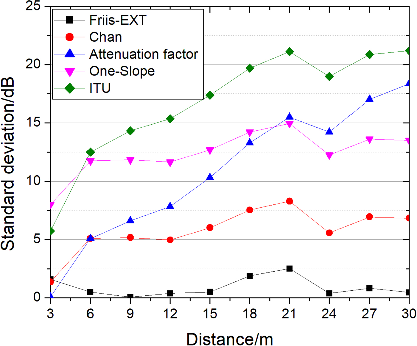
Fig. 7. The standard deviation of different models.
At each measurement point, the degree of deviation between the predicted value and the measured data is determined by solving the standard deviations of each model and measured data. Smaller standard deviation means less error, which reflects the accuracy of the model. From Figure 7, it can be realized that the standard deviation of Friis-EXT is the smallest, the Friis-EXT model is the best of these models and is a 5 dB improvement over the chan model at the most of measurement points except 3 m one.
Conclusion
A new path-loss model for an indoor multipath environment was proposed in this paper. The matching coefficient, polarization matching factor, and normalized field intensity direction function were considered in the modeling. When the matching coefficient τ, polarization matching factor cos(ξ), and normalized field intensity direction function F(θ, Φ) are equal to 1, the formula is consistent with Friis formula. In addition, reflective surfaces were added in the calculation process, and the specific environment and form of the antenna were considered. Furthermore, the data in the indoor corridor environment were measured, with antenna set at 0, 30, and 60° angles between the transmitting and receiving antennas. The errors were <7.5 dB. Finally, the Friis-EXT was compared with other traditional models. The results show that the Friis-EXT model matched the measured data best.
Author ORCIDs
Qiang Li, 0000-0003-2969-7844
Acknowledgements
The work was supported in part by the National Natural Science Foundation of China (No.61571063), and the Natural Science Foundation of Beijing Municipality (No.3182028), and the Science and technology project of State Grid Corporation of China (SGCC): Research and Chip Development of Broadband Power Line Carrier and Wireless Fusion Communication Technology.
Supplementary material
The supplementary material for this article can be found at https://doi.org/10.1017/S1759078719000084.
 Qiang Li (1985–), male, was born in Yingkou city of Liaoning province, China. He has received B.S. degree in communications engineering and M.S. degree in signal and information processing from Tianjin University of Technology and education in 2009 and 2012, respectively. Currently, he is working toward the Ph.D. degree in electronic science and technology at the Beijing University of Posts and Telecommunications. His recent research interests include electromagnetic compatibility and microwave technology, communications and signal processing. Email: qiang_lee@126.com
 Hongxin Zhang (1969–), male, was born in Binzhou city of Shandong province, China. Ph.D. professor, graduated from Beijing University of Posts and Telecommunications in 2004, and received Ph.D. degree, now he works as doctorial tutor in Beijing University of Posts and Telecommunications, and director of the center for broadband communications and microwave technology. Research direction: wireless communication and electromagnetic compatibility, communication signal processing, electromagnetic radiation, information security, biomedical engineering, etc. Email: hongxinzhang@263.net
 Yang Lu (1984–), male, was born in Xuzhou city of Jiangsu province, China. He graduated from Beijing University of Posts and Telecommunications in 2012, and received the Ph.D. degree, now he works as an engineer in Global Energy Internet Research Institute. Mainly engaged in research work on new technologies for power communication. E-mail: luyang@geiri.sgcc.com.cn
 Tianyi Zheng (1994–), female, was born in Beijing city of China. She has received her B.S. degree from Beijing University of Technology in 2016. Currently, she is pursuing M.S. in Beijing University of Posts and Telecommunications. She completed her B.S. in electronic engineering. Research direction: wireless communication, biomedical engineering. Email: zhengtianyi@bupt.edu.cn
 Yinghua Lv (1944–), male, was born in Jinzhou city of Liaoning province, China. Ph.D. professor, graduated from Beijing University of Posts and Telecommunications in 1988, and received the Ph.D. degree, now he works as a doctorial tutor in Beijing University of Post and Telecommunications. Research fields are computational electromagnetics, electromagnetic compatibility, biomedical engineering, antenna and the electromagnetic scattering, computer information technology, etc. Email: yhlu@bupt.edu.cn