2.1. Mean flow SP analysis

We begin by applying the SP analysis to a steady-state two-dimensional turbulent wake for which the mean momentum equation in the streamwise direction is given by

Here, $U$ , $V$ are the streamwise ( $x$ -direction) and lateral ( $y$ -direction) components of the mean velocity respectively; $\overline{u^{2}}$ , $\overline{v^{2}}$ and $\overline{uv}$ are the streamwise, lateral and shear stresses respectively. Following Townsend (Reference Townsend1956), we assume

where $U_{\infty }$ is the free stream velocity, $u_{0}$ and $v_{0}$ are scaling velocities which depend on $x$ and are not necessary identical, $y^{\ast }=y/l$ , $l$ being a scaling length which depends only on  $x$ . The functions $f$ , $g_{u}$ , $g_{v}$ and $g_{uv}$ are functions of $y^{\ast }$ only. Substituting expressions (2.2) into (2.1) and using the continuity equation ( $\boldsymbol{{\rm\nabla}}\boldsymbol{\cdot }U=0$ ) to solve for  $V$ , leads, after some trivial manipulations, to

where the prime and double prime denote first- and second-order derivatives with respect to $y^{\ast }$ respectively. Multiplying all the terms of (2.3) by $l/v_{0}^{2}$ makes the coefficient of $g_{uv}^{\prime }$ equal to 1, and, accordingly, SP is satisfied if

where the constants $C_{i}~(i=1\ldots 8)$ are independent of $x$ . Solving (2.4g ) yields

where we assumed that $l=0$ when $x=x_{0}$ ; $x_{0}$ is a virtual origin. However, by considering the ratio $C_{2}/C_{8}$ , we obtain

Clearly, (2.5) and (2.6) cannot be satisfied simultaneously.

Substituting (2.4g ) into (2.4b ), we have

Moreover, from (2.4b ) alone, we obtain

We can also have an SP constraint on $u_{0}$ by taking the ratio between (2.4a ) and (2.4c ). This leads to

Now, combining (2.7) and (2.9) yields

Then, substituting (2.10) into (2.4h ) leads to

Some discussion is required at this stage of the analysis. We note that the condition (2.8) is similar to that of George (Reference George, George and Arndt1989) for the Reynolds stress velocity scale. One can see that this constraint will also apply to a turbulent boundary layer, a jet flow and a mixing layer since the mean momentum in these flows obeys the same equation (2.1), which Townsend (Reference Townsend1956, Reference Townsend1976) used as the foundation for his SP analysis of different turbulent flows. In his analysis, George (Reference George, George and Arndt1989) only considered a first-order approximation form of (2.1) where the second and fourth terms of the left-hand side as well as the term on the right-hand side are removed. The approximation further assumes that $U\simeq U_{\infty }$ , and thus the first term of (2.1) can be replaced by $U_{\infty }(\partial U/\partial x)$ . This then removes the SP constraints (2.4d ), (2.4f – h ) from the analysis. It is believed that the first-order approximation of the mean momentum equation is valid in the far wake where the defect velocity can be considered to be very small, leading to $U\simeq U_{\infty }$ . Townsend (Reference Townsend1956) proposed that if $U_{\infty }/u_{0}\gg f$ in (2.3) then SP is possible in the plane wake. This condition leads to $C_{1}\gg C_{3}$ and, since $U_{\infty }u_{0}\,\text{d}l/\text{d}x=u_{o}\,\text{d}(U_{\infty }l)/\text{d}x$ , $C_{2}\gg C_{4}$ , and accordingly the third and fourth terms on the left-hand side of (2.3) can be dropped. Townsend (Reference Townsend1956) further assumed that the sixth, seventh and eighth terms can be neglected. At this stage of the analysis we do not make such simplifications.

It is worthwhile to comment on the consequence of dropping terms from (2.1). First, let us consider dropping the right-hand side, which, in effect, amounts to dropping the SP condition (2.4h ). This can only lead to the solution (2.5). If we drop the fourth term on the left-hand side of (2.1) and retain the right-hand side, SP solution (2.6) is obtained. If these terms are dropped (George Reference George, George and Arndt1989), one cannot predict the streamwise evolution of $l$ based on the mean momentum equation alone and is left with constraint (2.8). George (Reference George, George and Arndt1989) obtained this evolution by considering the momentum integral to first order, i.e. by assuming that the momentum integral is constant.

In the next section we apply the SP analysis to the s.b.s. energy budget, which will help us to obtain the appropriate streamwise evolution of  $l$ .

2.2. Scale-by-scale SP analysis

According to Danaila et al. (Reference Danaila, Anselmet, Zhou and Antonia2001), the s.b.s. energy budget equation on the axis of a plane far wake is given by

where $s$ is a dummy variable, identifiable with the separation along $x$ ; the $u_{i}~(i=1,2,3)$ represent the velocity fluctuations in the $x$ , $y$ and $z$ directions respectively. In this paper, $u_{1}$ , $u_{2}$ and $u_{3}$ will be used interchangeably with $u$ , $v$ , $w$ ; similarly for $x_{1}$ , $x_{2}$ , $x_{3}$ and $x$ , $y$ , $z$ . The first and second terms on the left-hand side of (2.12) are the large-scale forcing terms which arise from the transport of $({\rm\Delta}u_{i})^{2}$ by the mean velocity $U$ and the lateral velocity fluctuation $u_{2}$ , namely convection and turbulent diffusion respectively. The third term in (2.12) is the generalised third-order structure function (representing energy transfer between scales), while the fourth term represents the viscous diffusion. The term on the right-hand side of (2.12) is proportional to the energy dissipation rate and balances the sum of the other terms. Applying the limit at $r\rightarrow \infty$ yields the one-point kinetic energy budget, namely

We examine the conditions under which (2.12) satisfies SP at all scales by assuming the following functional forms for the terms in this equation:

where ${\it\xi}=r/l$ , ${\it\zeta}=y/{\it\delta}$ ; $l$ and ${\it\delta}$ are characteristic length scales in the $r$ and $y$ directions respectively; $u^{\ast }$ is a characteristic velocity scale. It should be noted that we assume only one velocity scale. Moreover, we do not presume any SP form for  $\overline{{\it\epsilon}}$ . The dimensionless functions $f({\it\xi},{\it\zeta})$ , $e({\it\xi},{\it\zeta})$ and $g({\it\xi},{\it\zeta})$ may depend on the initial conditions and are not considered here. After substituting expressions (2.14) into (2.12), we obtain the following SP s.b.s. equation:

where

It should be noted that the relations

have been used in deriving (2.15). After multiplication by $(l/{\it\nu}u^{\ast 2})$ , (2.15) becomes

If we express the mean velocity in terms of $U_{\infty }$ and the defect velocity $U_{d}$ , $U=U_{\infty }-U_{d}$ , (2.18) becomes

For SP, all of the terms within square brackets must evolve in the streamwise direction in exactly the same way. Since the last term on the left-hand side of (2.19) is constant, all of the others must also be constant, namely

Equation (2.20f ) indicates that in the far wake, the Reynolds number, based on the characteristic length and velocity scales ( $u^{\ast }$ and $l$ ), must remain constant.

The ratios of (2.20c ) to (2.20a ) and (2.20d ) to (2.20b ) lead to

i.e. $U_{d}/U_{\infty }$ must be constant for SP to be reached. However, since $U_{d}$ decreases as $x/d$ increases, one expects that $U_{d}/U_{\infty }\rightarrow 0$ as $x/d\rightarrow \infty$ . It is then reasonable to expect that $U_{d}/U_{\infty }\simeq 0$ beyond some downstream distance, such as in the far wake. In that case, $C_{3}$ and $C_{4}$ become negligible compared with $C_{1}$ and $C_{2}$ , and constraints (2.20c ) and (2.20d ) are no longer relevant and can be dropped from the analysis. Then, (2.20b ) leads to the following expression for the characteristic length scale  $l$ :

where $x_{0}$ is the effective flow origin and $c_{1}$ is a constant prefactor.

Equations (2.20a ) and (2.20g ) show that $u^{\ast }$ and $\bar{{\it\epsilon}}$ should behave as

and

It should be noted that (2.22)–(2.24) have been normalised by $d$ and $U_{\infty }$ . Equation (2.20e ) suggests that the characteristic length scale ${\it\delta}$ behaves like $l$ , namely

If one selects the half-width of the far wake, $L_{0}$ , as representing ${\it\delta}$ , then one expects $L_{0}\sim x^{1/2}$ .

A number of comments can be made based on the SP analyses shown above.

1. (i) Strictly, SP is reached exactly when the velocity defect $U_{d}$ is zero, which is likely to occur when $x/d\rightarrow \infty$ . However, if there is a region where $U_{d}\ll U_{\infty }$ , then SP solutions can be attained at some finite distance downstream of the cylinder. This is likely to occur in the far-wake region.

2. (ii) Equation (2.25) implies that ${\it\delta}\sim x^{1/2}$ , which shows that the SP constraint (2.4g ) on the mean momentum equation is not applicable, or, equivalently, the last term on the left-hand side of (2.3) is negligible and can be dropped from the SP analysis. It should be noted that this is different from dropping the fourth term on the left-hand side of (2.1).

3. (iii) Forming the ratio of (2.4c ) and (2.4a ) leads to $u_{o}/U_{\infty }$ . Townsend (Reference Townsend1956, Reference Townsend1976) assumed this ratio to be negligible and further dropped constraints (2.4f – h ), which amounts to using the first-order mean momentum equation,

   (2.26) $$\begin{eqnarray}U\frac{\partial U}{\partial x}+V\frac{\partial U}{\partial y}=-\frac{\partial \langle uv\rangle }{\partial y},\end{eqnarray}$$
   commonly used in the far wake. It should be noted that if one uses the Taylor hypothesis ( $x=Ut$ ) to convert space to time, then one obtains the temporally evolving plane wake. It appears that these simplifications are too restrictive. For example, there is no compelling justification for dropping the viscous term (e.g. the right-hand side term of (2.1)). In fact, retaining it leads, as seen in § 2.1, to the important constraint $\mathit{Re}_{l}=u_{0}l/{\it\nu}=\text{constant}$ , which is consistent with the SP constraint (2.20f ) applied to the s.b.s. budget.

4. (iv) If $l$ is identified with ${\it\lambda}$ and $u^{\ast }$ with $u^{\prime }$ , then $\mathit{Re}_{{\it\lambda}}=\text{const}$ . This is a convenient test for SP since $\mathit{Re}_{{\it\lambda}}$ is a relatively straightforward quantity to measure.

5. (v) Combining (2.20e ) and (2.20g ) yields

   (2.27) $$\begin{eqnarray}\frac{\bar{{\it\epsilon}}l}{u^{\ast 3}}=C_{8}.\end{eqnarray}$$
   If $l=L$ is the integral length scale and $u_{\ast }=u^{\prime }$ , then we obtain $C_{8}=C_{{\it\epsilon}}=\text{constant}$ , revealing that the constancy of $C_{{\it\epsilon}}$ is simply a consequence of SP.

We now follow the work of Thiesset, Antonia & Djenidi (Reference Thiesset, Antonia and Djenidi2014) and derive an exact expression for $\overline{{\it\epsilon}}$ using the SP solutions of the s.b.s. budget equation. As seen above, SP is reached when the defect velocity is negligible, which we assume at this stage to be well verified in the far wake. We thus focus the analysis on the far wake and seek to write the transport equation for the average kinetic energy $(\overline{q^{2}}=\overline{u_{i}^{2}})$ along the axis of the far wake. Several attempts have been made to measure the various terms of (2.13) in the far wake. For example, Browne et al. (Reference Browne, Antonia and Shah1987), Aronson & Lofdahl (Reference Aronson and Lofdahl1993) and Lefeuvre et al. (Reference Lefeuvre, Djenid, Antonia and Zhou2014) showed that, on the centreline of the far wake, the advection and diffusion terms (the first and second terms in (2.13) respectively) contribute significantly to the budget. Further, they found that the diffusion and advection terms are approximately equal, i.e.

Equation (2.13) can then be rewritten as

The turbulent kinetic energy along the axis of the far wake can be approximated by

where $R=\overline{u_{2}^{2}}/\overline{u_{1}^{2}}$ , which represents a measure of large-scale anisotropy; the approximation  $u_{2}^{2}\simeq u_{3}^{2}$ was used. This approximation is well supported by the measurements of Hao et al. (Reference Hao, Zhou, Chua and Yu2008) on the centreline of the far wake, where it was shown that $\overline{u_{1}^{2}}/\overline{u_{2}^{2}}\simeq \overline{u_{1}^{2}}/\overline{u_{3}^{2}}\simeq 1.4$ at $R_{d}=U_{\infty }d/{\it\nu}=2000$ . After substituting (2.24) and (2.30) in (2.29), we obtain

where $A_{u}$ is a power-law prefactor for $u^{\prime }$ . It should be noted that the condition that $U_{d}/U_{\infty }$ is negligible (see (2.21)) is also used in deriving (2.31), since we are focusing on the far wake.

Combining (2.31) with (2.24) yields an expression for $\overline{{\it\epsilon}}$ , namely

This expression provides a relatively simple method for estimating $\overline{{\it\epsilon}}$ , whose reliable measurement represents a challenge to the experimentalist. Indeed, it is sufficient to measure $\overline{u^{2}}$ and $R$ in order to estimate $\bar{{\it\epsilon}}$ .

It should be remembered that the departure from local isotropy in the far-wake region is not negligible, even on the flow centreline where the mean shear is zero (e.g. Antonia & Browne Reference Antonia and Browne1986; Browne et al. Reference Browne, Antonia and Shah1987). This departure can be quantified as follows:

Accordingly, (2.32) can be written as

It follows that the Kolmogorov velocity and length scales ( $u_{K}$ , ${\it\eta}$ ) should behave as

leading to

which is constant. Since $\overline{u^{\ast 2}}=\mathit{Re}_{{\it\lambda}}/\sqrt{15}$ , it follows that

Using the definition of the Taylor microscale ${\it\lambda}$ leads to

and

which is constant.

Figure 1. Schematic arrangement and coordinate axis. Here, $U$ is the mean velocity; $U_{\infty }$ is the free stream velocity; $U_{d}$ is the maximum velocity defect; $L_{0}$ is the half-width of the wake. It should be noted that $U$ and $U_{d}$ are arbitrarily shown on the centreline.

Similarly to the analysis of Thiesset et al. (Reference Thiesset, Antonia and Djenidi2014), the present SP analysis, applied to the s.b.s. budget equation, allows one to derive exact expressions for $\overline{u}^{2}$ , $\overline{{\it\epsilon}}$ and all subsequent quantities. In particular, relationships between the prefactors $A_{u}$ , $A_{{\it\lambda}}$ , $A_{\mathit{Re}_{{\it\lambda}}}$ and $c_{{\it\epsilon}}$ ensue. All of the results derived from the equilibrium similarity of the far wake are tested in §§ 4 and 5.

4.1. Mean velocity and Reynolds stresses

Constraints (2.9) and (2.21) show that one can use $u_{0}=U_{d}$ . Thus, the mean velocity defect $U_{\infty }^{+}-U^{+}$ , normalised with $U_{d}$ and $L_{0}$ , is shown in figure 2. Also shown are the data of Browne et al. (Reference Browne, Antonia and Shah1987) at $x/d=420$ . There is a reasonable collapse of the distributions for $U_{\infty }^{+}-U^{+}$ in the range $x/d>100$ between the present data and those of Browne et al. (Reference Browne, Antonia and Shah1987). As pointed out by Zhou & Antonia (Reference Zhou and Antonia1995), the distributions for $(U_{\infty }^{+}-U^{+})$ are approximately independent of the wake generators in the far-wake region of the plane wakes, although discernible differences can be observed in the Reynolds stresses, spectra of  $v$ and vorticities. For $x/d<100$ , discernible differences can be observed, especially near the outer edge of the wake. This is also consistent with the observations of Antonia & Mi (Reference Antonia and Mi1998) in the range $x/d\leqslant 70$ .

The r.m.s. of the streamwise fluctuations $u_{rms}^{+}$ , normalised with $U_{d}$ and $L_{0}$ , is shown in figure 3. Antonia & Mi (Reference Antonia and Mi1998) reported that the magnitude of $u_{rms}^{+}$ decreases as $x/d$ increases over the range $x/d=10{-}70$ . The same can be observed in figure 3. More importantly, the magnitude of $u_{rms}^{+}$ keeps decreasing as $x/d$ increases, eventually reaching a constancy beyond $x/d\approx 200$ . This suggests that SP is satisfied closely for $x/d>200$ , at least in the context of Reynolds stresses.

Figure 3. Normalised r.m.s. longitudinal velocity at $\mathit{Re}_{d}=2000$ , for $x/d=$ ♢, 20; ▫, 40; ▿, 60; ▵, 80; ◃, 100; ▹, 170; *, 211; $\bullet$ , 277; ●, 344; ▪, 401; ♦, 468; ▾, 534; ▴, 601. The solid curve corresponds to the cylinder far wake at $x/d=420$ (Browne et al. Reference Browne, Antonia and Shah1987).

4.2. Streamwise variation of scaling parameters

The scaling parameters, $U_{d}$ and $L_{0}$ , clearly provide the collapse of the mean velocity profiles and the r.m.s. longitudinal velocity, as shown in figures 2 and 3. From the s.b.s. SP analysis, we show that any velocity scale must decay as $x^{-1/2}$ whereas any length scale must grow as $x^{1/2}$ . For $U_{d}$ and $L_{0}$ , namely

Figure 4. Downstream evolution of $U_{d}$ and $L_{0}$ at $\mathit{Re}_{d}=2000$ . The solid lines are the linear fits over the ranges $x/d=260{-}600$ and $x/d=20{-}100$ respectively.

The streamwise variations of $U_{d}$ and $L_{0}$ are shown in figure 4. A least-squares linear fit has been applied to the distributions of $(U_{\infty }/U_{d})^{2}$ and $(L_{0}/d)^{2}$ over the range $x/d=260{-}600$ . It is clear that the present data support the results from the above s.b.s. SP analysis over the range $x/d>260$ , where both $(U_{\infty }/U_{d})^{2}$ and $(L_{0}/d)^{2}$ grow linearly. The estimated values for $C_{1}$ and $C_{2}$ , which are 1.11 and 0.21 respectively, are in good agreement with those of Wygnanski et al. (Reference Wygnanski, Champagne and Marasli1986) ( $C_{1}=1.24$ and $C_{2}=0.20$ ), Browne & Antonia (Reference Browne and Antonia1986), Browne et al. (Reference Browne, Antonia and Shah1987) ( $C_{1}=1.28$ and $C_{2}=0.20$ ) and Aronson & Lofdahl (Reference Aronson and Lofdahl1993) ( $C_{1}=1.25$ and $C_{2}=0.20$ ), although they may depend on the initial conditions, as reported by (Wygnanski et al. Reference Wygnanski, Champagne and Marasli1986). Interestingly, there is also a linear evolution for both $(U_{\infty }/U_{d})^{2}$ and $(L_{0}/d)^{2}$ over the range $x/d=20{-}100$ (a least-squares linear fit has also been applied over this range). This is consistent with Mi, Zhou & Nathan (Reference Mi, Zhou and Nathan2004). Indeed over the range $x/d=20{-}100$ , both the mean temperature and the r.m.s. temperature on the wake axis decay as $x^{-1/2}$ , while the half-widths of the mean velocity and scalar fields grow as $x^{1/2}$ . A linear evolution for $(U_{\infty }/U_{d})^{2}$ and $(L_{0}/d)^{2}$ is also observed in a square cylinder wake over the range $x/d=30{-}100$ (DNS data of Lefeuvre, private communication, 2014) at $\mathit{Re}_{d}=2000$ . Figure 4 shows that the rates of change with $x$ of $(U_{\infty }/U_{d})^{2}$ and $(L_{0}/d)^{2}$ are smaller in the far wake than over the range $x/d=20{-}100$ (intermediate wake). This is more pronounced for $(L_{0}/d)^{2}$ than for $(U_{\infty }/U_{d})^{2}$ . The change of the rates from the ranges $x/d=20{-}100$ to $x/d=260{-}600$ seems to be an effect of the reorganisation or rescaling of the large-scale structures (Brown & Roshko Reference Brown and Roshko2012), which occurs over the range $x/d=100{-}260$ . This reorganisation or rescaling depends on the initial conditions. Figure 4 shows that the turbulent wake of a circular cylinder evolves through three stages, i.e. two linear evolution stages over the ranges $x/d=20{-}100$ and 260–600, and a transition stage over the range $100\leqslant x/d\leqslant 260$ , where the upstream and downstream limits depend on the ICs. Moreover, based on the results for a circular cylinder, only two basic regions are recognised by Brown & Roshko (Reference Brown and Roshko2012) over the range $4\leqslant x/d\leqslant 1000$ , namely the intermediate wake $(4\leqslant x/d\leqslant 50)$ and the far wake $(50\leqslant x/d\leqslant 1000)$ . This different classification is, in essence, due to the fact that different criteria are used. Brown & Roshko (Reference Brown and Roshko2012) showed that, in the intermediate wake, the presence of vortices shed from the cylinder is detectable, whereas in the far wake, there is approximately self-similar behaviour of the mean velocity, as shown in figure 2. The present classification is based on the streamwise evolution of the scaling parameters $U_{d}$ and $L_{0}$ . The transition region $100\leqslant x/d\leqslant 260$ is certainly worthy of further investigation. A further worthwhile issue to be investigated is the effect of the individual contributions from the energetic coherent structures and the velocity defect on the establishment of SP in the far wake, in particular on the limit of validity of SP on $x/d$ . Both of these features are dependent on the initial conditions. A possible way to assess the effects of the energetic coherent structures, which are likely to impact strongly on the wake flow evolution in the near-wake region, would be to systematically vary the Reynolds number for a given bluff body shape. The effect of the velocity defect could be assessed by varying the shape of the bluff body for a fixed Reynolds number, or, alternatively, by using a bluff body with different rear base bleeds. Interestingly, this latter approach amounts to assessing the effect of the drag on the establishment of SP. However, since the velocity defect reflects the force drag, one must be careful when using the estimate of the drag based on the momentum integral for assessing the SP results. For example, estimates of the drag based on the first-order momentum integral (valid in the far wake only) will result in inconsistency with SP in regions where the velocity defect is not negligible, such as in the near-wake field.

The local Reynolds number based on $U_{d}$ and $L_{0}$ , $\mathit{Re}_{0}=U_{d}L_{0}/{\it\nu}$ , is shown in figure 5. As expected from the s.b.s. SP analysis, $\mathit{Re}_{0}$ is constant for $x/d>260$ . By contrast, although both $(U_{\infty }/U_{d})^{2}$ and $(L_{0}/d)^{2}$ grow linearly over the range $x/d=20{-}100$ , $\mathit{Re}_{0}$ increases continuously instead of remaining constant. This is because different values of the virtual origin ( $x_{0}$ ) apply to $(U_{\infty }/U_{d})^{2}$ and $(L_{0}/d)^{2}$ over the range $x/d=20{-}100$ (it is clear in figure 4 that there is an intersection at $x/d\approx 40$ ), whereas in the far wake, the values of $x_{0}$ , estimated from $(U_{\infty }/U_{d})^{2}$ and $(L_{0}/d)^{2}$ , are approximately equal (this will be discussed in the next paragraph). Over the transition stage ( $100\leqslant x/d\leqslant 260$ ), $\mathit{Re}_{0}$ decreases continuously.

Figure 5. Downstream evolution of the local Reynolds number $\mathit{Re}_{0}$ at $\mathit{Re}_{d}=2000$ . The solid line is the mean value of $\mathit{Re}_{0}$ over the range $x/d=260{-}600$ .

Figure 6. Downstream evolution of ${\it\lambda}$ and $u^{\prime }$ at $\mathit{Re}_{d}=2000$ . The solid lines are the linear fits over the range $x/d=200{-}600$ .

Figure 7. Downstream evolution of ${\it\eta}$ at $\mathit{Re}_{d}=2000$ . The solid line is the linear fit over the range $x/d=200{-}600$ . For the purpose of comparison, we also show the values of $x_{0}$ for different quantities: $(U_{\infty }/U_{d})^{2}$ , ♢; $(L_{0}/d)^{2}$ , ●; $({\it\lambda}/d)^{2}$ , $+$ ; $(U_{\infty }/u_{rms})^{2}$ , $\times$ ; $({\it\eta}/d)^{2}$ , ◃.

Figure 8. Downstream evolution of the Taylor Reynolds number $\mathit{Re}_{{\it\lambda}}$ at $\mathit{Re}_{d}=2000$ . The solid line indicates the mean value of $\mathit{Re}_{{\it\lambda}}$ over the range $x/d=200{-}600$ .

The streamwise variations of $({\it\lambda}/d)^{2}$ , $(U_{\infty }/u_{rms})^{2}$ and $({\it\eta}/d)^{2}$ are shown in figures 6 and 7. All three quantities vary smoothly over the range $x/d=20{-}200$ , before increasing linearly for $x/d>200$ . The solid lines in figures 6 and 7 are linear fits over the range $x/d=200{-}600$ . Like the local Reynolds number $\mathit{Re}_{0}$ in figure 5, the Taylor microscale Reynolds number $\mathit{Re}_{{\it\lambda}}$ , shown in figure 8, reaches a constant value beyond $x/d\simeq 200$ , implying that SP is satisfied closely. Several further comments can be made with regard to figures 4–8.

(i) Self-preservation is achieved approximately in the far wake (beyond $x/d>260$ for all statistics) of a circular cylinder, indicating that all length scales ( $L_{0}$ , ${\it\lambda}$ , or ${\it\eta}$ ) and velocity scales ( $U_{d}$ , $u_{rms}$ or $u_{K}$ ) behave similarly, i.e. all velocity scales decay as $x^{-1/2}$ , whereas the length scales grow as $x^{1/2}$ , or the Reynolds numbers, based on any characteristic set of length and velocity scales, are constant. This feature of the far-wake region allows one to use all of the length and velocity scales interchangeably when scaling the data, e.g. the energy structure functions and spectra collapse over the entire range of scales/wavenumbers when normalised by any set of length and velocity scales; this will be discussed in the next section.

(ii) As the flow evolves from the near-wake field to the far-wake field, the statistics associated with the large-scale motion (LSM) approach SP at a lower rate than those associated with the small-scale motion. This is reflected by the fact that $\mathit{Re}_{{\it\lambda}}$ (see figure 8) reaches a constant faster than $\mathit{Re}_{0}$ (see figure 5). It is also reflected by the ratios of all length scales (i.e.  $L_{0}/{\it\eta}$ , ${\it\lambda}/{\it\eta}$ and $L_{0}/{\it\lambda}$ , not shown here) and all velocity scales (i.e.  $U_{d}/U_{k}$ , $u_{rms}/U_{K}$ and $U_{d}/u_{rms}$ , not shown). Namely, to become constant, the ratios associated with the large scales (i.e.  $L_{0}/{\it\eta}$ , $L_{0}/{\it\lambda}$ , $U_{d}/U_{k}$ and $U_{d}/u_{rms}$ ) require longer downstream distances than the ratios associated with the small scales ( ${\it\lambda}/{\it\eta}$ and $u_{rms}/U_{K}$ ).

(iii) In the s.b.s. SP analysis we assumed that $x_{0}$ associated with the different length scales ( $L_{0}$ , ${\it\lambda}$ , or ${\it\eta}$ ) and velocity scales ( $U_{d}$ , $u_{rms}$ or $u_{K}$ ) is identical. To test this assumption, we marked the values of $x_{0}$ for all quantities in figure 7 at $\mathit{Re}_{d}=2000$ . They are approximately equal ( ${\approx}-25d$ ). For comparison, we reproduce the values of $x_{o}$ measured in other cylinder wakes and reported in the literature. For example, Browne & Antonia (Reference Browne and Antonia1986) and Browne et al. (Reference Browne, Antonia and Shah1987) estimated $x_{0}\approx -125d$ at $\mathit{Re}_{d}=1170$ ; Aronson & Lofdahl (Reference Aronson and Lofdahl1993) obtained $x_{0}\approx -112d$ at $\mathit{Re}_{d}=1840$ ; Sreenivasan (Reference Sreenivasan1981) measured $x_{0}\approx -70d$ at $\mathit{Re}_{d}=1160$ . The present value of $x_{o}$ differs significantly from that of Aronson & Lofdahl (Reference Aronson and Lofdahl1993) although the Reynolds numbers are not too dissimilar. This is also observed between Sreenivasan (Reference Sreenivasan1981) and Browne & Antonia (Reference Browne and Antonia1986), Browne et al. (Reference Browne, Antonia and Shah1987). This suggests that the initial conditions have a more important effect on $x_{o}$ than the Reynolds number.

4.3. A simple means for estimating $\bar{{\it\epsilon}}$

Equation (2.32) provides a simple means for estimating $\bar{{\it\epsilon}}$ along the wake axis once $\overline{u^{2}}$ and $R$ are known. Before checking the accuracy of the present estimates for $\bar{{\it\epsilon}}$ with (2.32), the spectral chart method of Djenidi & Antonia (Reference Djenidi and Antonia2012) has been applied to the present spectra as an attempt to obtain more accurate values of the energy dissipation rate, when plotted in the form ${\it\phi}_{u}(f)$ versus  $f$ . The ‘new’ estimates of $\bar{{\it\epsilon}}$ are denoted by $\bar{{\it\epsilon}}_{spec}$ . In essence, these values ensure that there is collapse in the upper part of the dissipative range. Since this collapse has a solid analytical underpinning (we recall here that the LI assumption was relaxed in Antonia, Djenidi & Danaila (Reference Antonia, Djenidi and Danaila2014) to an assumption of local axisymmetry), $\bar{{\it\epsilon}}_{spec}$ should be very close to the true value of $\bar{{\it\epsilon}}$ . Figure 9 shows the distribution of ${\it\phi}_{u}^{\ast }(k_{1}^{\ast })$ for several positions over the range $200<x/d<600$ . The red curves are normalised by $\bar{{\it\epsilon}}_{iso}$ and ${\it\nu}$ , while the blue curves are normalised by $\bar{{\it\epsilon}}_{spec}$ and  ${\it\nu}$ . Moreover, for reference, the velocity spectrum on the centreline of a fully developed channel flow is shown (Abe, Antonia & Kawamura Reference Abe, Antonia and Kawamura2009). There is a very good agreement between the ‘ $\bar{{\it\epsilon}}_{spec}$ ’-normalised spectra and the channel flow spectrum. On the other hand, the spectra normalised by $\bar{{\it\epsilon}}_{iso}$ and ${\it\nu}$ are shifted up, suggesting that $\bar{{\it\epsilon}}_{iso}$ differs from the actual $\bar{{\it\epsilon}}$ ( $\simeq \,\bar{{\it\epsilon}}_{spec}$ ). In this case, the ratio $R_{{\it\epsilon}}=\bar{{\it\epsilon}}_{iso}/\bar{{\it\epsilon}}_{spec}$ is 0.75. We recall that Aronson & Lofdahl (Reference Aronson and Lofdahl1993) measured the diffusion and advection terms for the one-point kinetic energy budget (2.13), as well as the isotropic dissipation rate $\bar{{\it\epsilon}}_{iso}$ in the far wake of a circular cylinder at a comparable $\mathit{Re}_{d}$ ( $=1840$ ). Thus, $R_{{\it\epsilon}}$ can be estimated as follows:

which is quite close to the value of 0.75 estimated by the spectral chart method at $\mathit{Re}_{d}=2000$ .

Now, we estimate $\bar{{\it\epsilon}}$ with (2.32). At $\mathit{Re}_{d}=2000$ , Hao et al. (Reference Hao, Zhou, Chua and Yu2008) showed that both $\overline{u_{1}^{2}}/\overline{u_{2}^{2}}$ and $\overline{u_{1}^{2}}/\overline{u_{3}^{2}}$ are approximately 1.4 on the centreline of the far wake. Namely $R=0.71$ at $\mathit{Re}_{d}=2000$ . Estimates of $\bar{{\it\epsilon}}$ from (2.32) are shown in figure 10 with $A_{u}=0.318$ , $x_{0}=-22d$ and $R=0.71$ ( $A_{u}$ and $x_{0}$ are estimated from the present data). Also shown are the values of $\bar{{\it\epsilon}}_{iso}$ . The estimated value of $R_{{\it\epsilon}}$ from this figure is approximately 0.75 (the square symbols for $\bar{{\it\epsilon}}_{iso}/0.75$ collapse reasonably well with $\bar{{\it\epsilon}}$ ), which is in good agreement with the estimate from the spectral chart method above, confirming that (2.32) provides a good and reliable estimate of  $\bar{{\it\epsilon}}$ .

Figure 9. Kolmogorov normalised spectra of $u$ over the range $x/d=200{-}600$ at $\mathit{Re}_{d}=2000$ . The red curves are normalised by $\bar{{\it\epsilon}}_{iso}$ and ${\it\nu}$ , while the blue curves are normalised by $\bar{{\it\epsilon}}_{spec}$ (the spectral chart method) and  ${\it\nu}$ . The black curve corresponds to the spectrum of  $u$ on the centreline of a fully developed channel flow (Abe et al. Reference Abe, Antonia and Kawamura2009).

Figure 10. Evolution along the centreline of $\bar{{\it\epsilon}}$ at $\mathit{Re}_{d}=2000$ : ○, measured $\bar{{\it\epsilon}}_{iso}$ ; ▫, measured $\bar{{\it\epsilon}}_{iso}/0.75$ . The red line is calculated from (2.32) with $A_{u}=0.318$ , $x_{0}=-22d$ and $R=0.71$ .

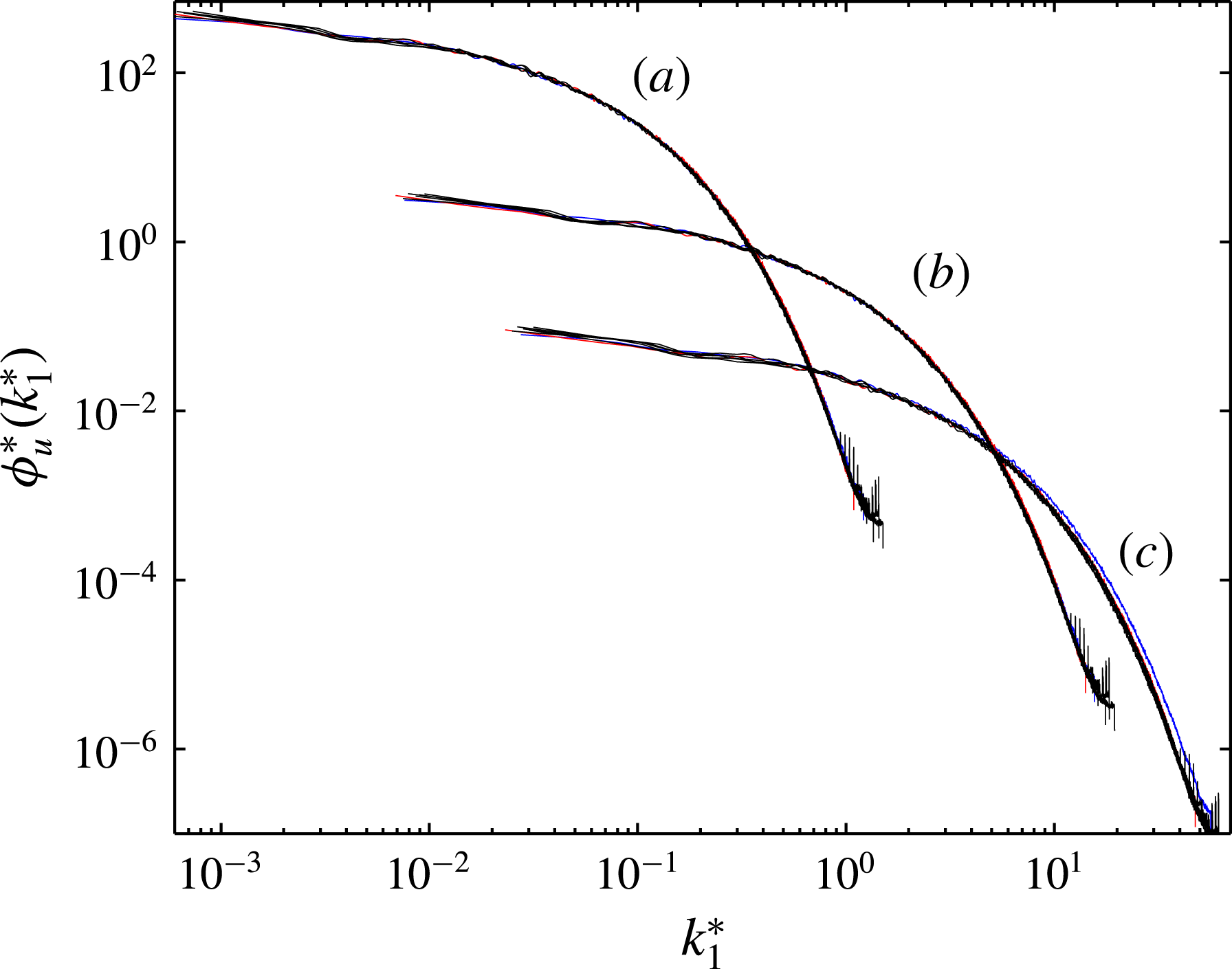
Figure 11. Spectra of $u$ over the range $x/d=200{-}600$ ( $x/d=211$ (blue), 277, 344, 401, 468, 534 and 601) at $\mathit{Re}_{d}=2000$ , normalised by (a) Kolmogorov scales, (b)  ${\it\lambda}$ and $u^{\prime }$ , (c)  $U_{d}$ and  $L_{0}$ .

In addition, the predicted value for $A_{\mathit{Re}_{{\it\lambda}}}$ from (2.38) is 0.92, which is also in agreement with the experimental value of 0.96 at $\mathit{Re}_{d}=2000$ . Since, as noted in the introduction, there is abundant evidence to indicate that the SP depends on the ICs, the ratios $A_{\mathit{Re}_{{\it\lambda}}}$ , $A_{u}$ and $c_{{\it\epsilon}}$ should also depend on the ICs. Indeed, as pointed out by Antonia, Zhou & Romano (Reference Antonia, Zhou and Romano2002), although the ratio $A_{\mathit{Re}_{{\it\lambda}}}$ (or $\mathit{Re}_{{\it\lambda}}/\mathit{Re}_{d}^{1/2}$ ) is approximately independent of $\mathit{Re}_{{\it\lambda}}$ at $x/d=70$ in wakes generated by five different bluff bodies (i.e. a solid circular cylinder, a circular cylinder constructed from a screen of 54 % solidity, a solid square cylinder, a solid plate placed normal to the flow and a screen strip, over a range of Reynolds numbers), its magnitude varies significantly between the wakes at the same  $\mathit{Re}_{d}$ .