


1 Introduction
Unsteady thrust generation by fishes and other underwater organisms have long been of interest to engineers (Lighthill Reference Lighthill1970). This desire to understand the propulsion mechanisms of fish has gained importance recently due to the possibilities of designing novel bio-inspired propulsors using such unsteady mechanisms (Lauder et al. Reference Lauder, Madden, Tangorra, Anderson and Baker2011; Low Reference Low2011). Fish fins and wings of birds are known to be flexible (Combes & Daniel Reference Combes and Daniel2003), with passive deformations of fins and wings occurring during flapping. The early studies of Wu (Reference Wu1971) and Katz & Weihs (Reference Katz and Weihs1978) showed that flexible bodies can achieve higher propulsive efficiencies than their rigid counterparts. This possibility of higher propulsive efficiency has motivated recent work investigating the effects of flexibility on the flow field and forces of flapping flexible panels and foils (see for example, Heathcote & Gursul Reference Heathcote and Gursul2007; Michelin & Llewellyn Smith Reference Michelin and Llewellyn Smith2009; Kang et al. Reference Kang, Aono, Cesnik and Shyy2011; Dewey et al. Reference Dewey, Boschitsch, Moored, Stone and Smits2013). There have however been very few experimental studies on flexible flapping foils with measurements of efficiency (Heathcote & Gursul Reference Heathcote and Gursul2007; Dewey et al. Reference Dewey, Boschitsch, Moored, Stone and Smits2013; Quinn, Lauder & Smits Reference Quinn, Lauder and Smits2014), and only one for the case of a flexible pitching panel (Dewey et al. Reference Dewey, Boschitsch, Moored, Stone and Smits2013). In the present work, we investigate through direct force measurements the thrust generation from a pitching rigid foil with a flexible trailing edge flap, the flap length and flexibility being the parameters that are varied. The thrust and the propulsive efficiency are both directly measured along with the wake velocity field. Apart from the study of Dewey et al. (Reference Dewey, Boschitsch, Moored, Stone and Smits2013), where a pitching panel which is flexible along its complete length was studied, there have been no prior experimental studies of pitching flexible panels/foils with measurements of efficiency.
Thrust generation from rigid oscillating foils in a free stream has been extensively studied as reviewed by McCroskey (Reference McCroskey1982), Shyy et al. (Reference Shyy, Aono, Chimakurthi, Trizila, Kang, Cesnik and Liu2010) and Platzer et al. (Reference Platzer, Jones, Young and Lai2008). This includes pure heaving studies (for example, Wang Reference Wang2000; Lewin & Haj-Hariri Reference Lewin and Haj-Hariri2003), pure pitching studies (for example, Godoy-Diana, Aider & Wesfreid Reference Godoy-Diana, Aider and Wesfreid2008; Bohl & Koochesfahani Reference Bohl and Koochesfahani2009; Mackowski & Williamson Reference Mackowski and Williamson2015) or a combination of both (Anderson et al.
Reference Anderson, Streitlien, Barrett and Triantafyllou1998). Propulsive efficiencies have also been investigated, both numerically and experimentally, although there have been only a few experimental studies where these have been directly measured (Anderson et al.
Reference Anderson, Streitlien, Barrett and Triantafyllou1998; Buchholz & Smits Reference Buchholz and Smits2008; Dewey et al.
Reference Dewey, Boschitsch, Moored, Stone and Smits2013; Mackowski & Williamson Reference Mackowski and Williamson2015). For a rigid foil in both pitch and heave with a phase angle between the pitch and heave of approximately
 $90\,^{\circ }$
, Anderson et al. (Reference Anderson, Streitlien, Barrett and Triantafyllou1998) reported efficiencies of up to 87 %. On the other hand, in purely pitching cases, Buchholz & Smits (Reference Buchholz and Smits2008) report much lower peak propulsive efficiencies of 9 %–21 % for finite span panels, while Mackowski & Williamson (Reference Mackowski and Williamson2015) report peak efficiencies of approximately 12 % for a pitching NACA 0012 foil.
$90\,^{\circ }$
, Anderson et al. (Reference Anderson, Streitlien, Barrett and Triantafyllou1998) reported efficiencies of up to 87 %. On the other hand, in purely pitching cases, Buchholz & Smits (Reference Buchholz and Smits2008) report much lower peak propulsive efficiencies of 9 %–21 % for finite span panels, while Mackowski & Williamson (Reference Mackowski and Williamson2015) report peak efficiencies of approximately 12 % for a pitching NACA 0012 foil.
The effects of panel/foil flexibility on the flow and forces have recently been investigated both analytically and numerically (Michelin & Llewellyn Smith Reference Michelin and Llewellyn Smith2009; Eldredge, Toomey & Medina Reference Eldredge, Toomey and Medina2010; Kang et al. Reference Kang, Aono, Cesnik and Shyy2011; Dai et al. Reference Dai, Luo, Ferreira De Sousa and Doyle2012; Paraz, Schouveiler & Eloy Reference Paraz, Schouveiler and Eloy2016), and experimentally (Prempraneerach, Hover & Triantafyllou Reference Prempraneerach, Hover and Triantafyllou2004; Heathcote & Gursul Reference Heathcote and Gursul2007; Marais et al. Reference Marais, Thiria, Wesfreid and Godoy-Diana2012; Dewey et al. Reference Dewey, Boschitsch, Moored, Stone and Smits2013; Paraz, Eloy & Schouveiler Reference Paraz, Eloy and Schouveiler2014; Quinn et al. Reference Quinn, Lauder and Smits2014; Shinde & Arakeri Reference Shinde and Arakeri2014). Eldredge et al. (Reference Eldredge, Toomey and Medina2010) and Shinde & Arakeri (Reference Shinde and Arakeri2014) have investigated the effects of a flapping flexible foil/panel in the absence of a free stream. Most of the other studies investigate the effects of a heaving flexible panel in the presence of a free stream, and broadly report enhanced propulsive efficiencies for an optimally flexible panel, with nearly the entire chord length of the panel being flexible in the majority of these studies.
Oscillation of the flexible panel/foil at near its natural frequency has been reported to be beneficial in a number of studies, the natural frequency being determined in many cases as the frequency at which the tip amplitude deflection is maximum. In some cases, this resonance has been linked to maximum thrust production (Heathcote & Gursul Reference Heathcote and Gursul2007; Michelin & Llewellyn Smith Reference Michelin and Llewellyn Smith2009; Kang et al. Reference Kang, Aono, Cesnik and Shyy2011; Paraz et al. Reference Paraz, Schouveiler and Eloy2016), with the optimal propulsive efficiency occurring at a fraction of such a natural frequency, while in others it has been linked to the optimal efficiency condition (Dewey et al. Reference Dewey, Boschitsch, Moored, Stone and Smits2013; Quinn et al. Reference Quinn, Lauder and Smits2014). In contrast, there have also been studies that suggest that optimization of performance occurs not necessarily by achieving larger flapping amplitudes through resonance, but through fluid mechanical tuning of the foil/panel shape (Ramananarivo, Godoy-Diana & Thiria Reference Ramananarivo, Godoy-Diana and Thiria2011) or where the optimal efficiency occurs well below the resonant frequencies (Vanella et al. Reference Vanella, Fitzgerald, Preidikman, Balaras and Balachandran2009; Kang et al. Reference Kang, Aono, Cesnik and Shyy2011). We shall see in the present case of a pitching rigid foil with a flexible trailing edge flap that there is a clear and distinct mode shape associated with both the optimal thrust and optimal efficiency condition suggesting similarities with the study of Michelin & Llewellyn Smith (Reference Michelin and Llewellyn Smith2009) and Ramananarivo et al. (Reference Ramananarivo, Godoy-Diana and Thiria2011).
The wake vortex dynamics behind flapping foils has also been extensively investigated. Wake patterns for purely pitching rigid foils at low pitching angles were reported by Koochesfahani (Reference Koochesfahani1989) and detailed measurements in the wake of pitching foils at low pitching angles and high reduced frequency were reported by Bohl & Koochesfahani (Reference Bohl and Koochesfahani2009). Godoy-Diana et al. (Reference Godoy-Diana, Aider and Wesfreid2008) and Schnipper, Andersen & Bohr (Reference Schnipper, Andersen and Bohr2009) mapped out different wake patterns as a function of the trailing edge amplitude and frequency for such pitching rigid foils. They found a variety of different wake vortex configurations including the Kármán street, reverse Kármán street and asymmetric wakes that are deflected at an angle to the free stream. Marais et al. (Reference Marais, Thiria, Wesfreid and Godoy-Diana2012) and Shinde & Arakeri (Reference Shinde and Arakeri2014) showed that foil flexibility inhibits the asymmetric wake mode.
Of all the prior studies involving pitching motion, the only direct measurements of propulsive efficiency from flexible pitching panels is the recent work of Dewey et al. (Reference Dewey, Boschitsch, Moored, Stone and Smits2013), where panels of varying stiffness where pitched downstream of a stationary fairing. In the present experiments, a rigid foil of chord length
 $c_{R}$
is pitched with a flexible trailing edge flap of length
$c_{R}$
is pitched with a flexible trailing edge flap of length
 $c_{F}$
and its thrust and propulsive efficiencies are measured. In this case, the attachment point of the flexible flap moves laterally to the free stream in addition to pitching, which could be thought of as a combination of heave and pitch for the flexible flap. The rigid part of the foil in our case is a NACA 0012 foil that is pitched about its quarter chord with pitching amplitude of
$c_{F}$
and its thrust and propulsive efficiencies are measured. In this case, the attachment point of the flexible flap moves laterally to the free stream in addition to pitching, which could be thought of as a combination of heave and pitch for the flexible flap. The rigid part of the foil in our case is a NACA 0012 foil that is pitched about its quarter chord with pitching amplitude of
 $10\,^{\circ }$
, while the flexural rigidity (
$10\,^{\circ }$
, while the flexural rigidity (
 $EI$
) of the aft flexible flap is varied over a large range of values. The flexible flap length (
$EI$
) of the aft flexible flap is varied over a large range of values. The flexible flap length (
 $c_{F}$
) has also been systematically varied in our experiments, which we quantify using the ratio of the flexible flap length to total chord length ratio (
$c_{F}$
) has also been systematically varied in our experiments, which we quantify using the ratio of the flexible flap length to total chord length ratio (
 $c_{F}/c$
), where the total chord length
$c_{F}/c$
), where the total chord length
 $c$
is the sum of
$c$
is the sum of
 $c_{R}$
and
$c_{R}$
and
 $c_{F}$
. We shall refer to this combination foil as a flexible foil with total chord length
$c_{F}$
. We shall refer to this combination foil as a flexible foil with total chord length
 $c$
in this work. A schematic of the reference rigid foil and flexible foil studied in the present experiments is shown in figure 1 along with the main parameters in the problem.
$c$
in this work. A schematic of the reference rigid foil and flexible foil studied in the present experiments is shown in figure 1 along with the main parameters in the problem.

Figure 1. Schematic showing the parameters involved in (a) rigid and (b) flexible foils undergoing pitching oscillations in a uniform flow. In (a), a rigid foil of chord
 $c$
undergoes sinusoidal pitching oscillations with angular amplitude
$c$
undergoes sinusoidal pitching oscillations with angular amplitude
 $\unicode[STIX]{x1D703}_{max}$
and frequency
$\unicode[STIX]{x1D703}_{max}$
and frequency
 $f$
about its quarter chord point. In (b), the flexible foil is shown, which comprises a flexible flap of length
$f$
about its quarter chord point. In (b), the flexible foil is shown, which comprises a flexible flap of length
 $c_{F}$
and flexural rigidity
$c_{F}$
and flexural rigidity
 $EI$
attached to a rigid chord of length
$EI$
attached to a rigid chord of length
 $c_{R}$
, which together combine to form the total chord
$c_{R}$
, which together combine to form the total chord
 $c$
. This flexible foil is again pitched about the quarter chord point of the rigid foil with angular amplitude
$c$
. This flexible foil is again pitched about the quarter chord point of the rigid foil with angular amplitude
 $\unicode[STIX]{x1D703}_{max}$
and frequency
$\unicode[STIX]{x1D703}_{max}$
and frequency
 $f$
.
$f$
.
In the present work, the total thrust generated by rigid and flexible foils is determined from measurements of the normal (
 $N$
) and axial or chordwise forces (
$N$
) and axial or chordwise forces (
 $A$
) acting on the purely pitching foil, the normal and axial being defined with respect to the rigid part of the foil in the flexible cases. This is achieved by mounting the load cell in a rotating reference frame along with the foil. This measurement of both normal and chordwise forces enables us to comment on the role of each of these two forces in the mean thrust (
$A$
) acting on the purely pitching foil, the normal and axial being defined with respect to the rigid part of the foil in the flexible cases. This is achieved by mounting the load cell in a rotating reference frame along with the foil. This measurement of both normal and chordwise forces enables us to comment on the role of each of these two forces in the mean thrust (
 $\overline{T}$
) generated. Simultaneous moment measurement allows us to calculate the mean input power (
$\overline{T}$
) generated. Simultaneous moment measurement allows us to calculate the mean input power (
 $\overline{P}$
) required to oscillate the foil and hence to calculate the propulsive efficiency (
$\overline{P}$
) required to oscillate the foil and hence to calculate the propulsive efficiency (
 $\unicode[STIX]{x1D702}=\overline{T}U/\overline{P}$
, where
$\unicode[STIX]{x1D702}=\overline{T}U/\overline{P}$
, where
 $U$
is free-stream velocity). Although there have been many studies on different aspects of oscillating foils, there have been no direct experimental measurements of thrust and propulsive efficiency of a flexible pitching foil that has only some portion of the total foil being flexible. As we shall see, even the addition of a relatively small flexible flap of appropriate stiffness can significantly change the thrust and propulsive efficiency characteristics of the pitching foil.
$U$
is free-stream velocity). Although there have been many studies on different aspects of oscillating foils, there have been no direct experimental measurements of thrust and propulsive efficiency of a flexible pitching foil that has only some portion of the total foil being flexible. As we shall see, even the addition of a relatively small flexible flap of appropriate stiffness can significantly change the thrust and propulsive efficiency characteristics of the pitching foil.
The paper is organized as follows. In § 2, we give an overview of the various experimental techniques used. The forces and the thrust characteristics of the rigid foil are briefly presented in § 3. The flexible foil results comprising the flap deflections and the force measurements are presented in § 4. We present here the effects of variations in oscillation frequency (
 $f$
), flexural rigidity (
$f$
), flexural rigidity (
 $EI$
) and the flexible flap to total chord length ratio (
$EI$
) and the flexible flap to total chord length ratio (
 $c_{F}/c$
) on thrust and efficiency. Results from particle image velocimetry (PIV) measurements in the wake of both rigid and flexible foils are presented in § 5. This is followed by discussions in § 6 after which the conclusions are presented in § 7.
$c_{F}/c$
) on thrust and efficiency. Results from particle image velocimetry (PIV) measurements in the wake of both rigid and flexible foils are presented in § 5. This is followed by discussions in § 6 after which the conclusions are presented in § 7.
2 Experimental method
The experimental set-up consists of a rigid NACA 0012 foil of chord length,
 $c_{R}=10~\text{cm}$
, pitched sinusoidally by a AC servo motor (Panasonic, Minas A4), as shown in figure 2(a). The motor gets its sinusoidal driving signal,
$c_{R}=10~\text{cm}$
, pitched sinusoidally by a AC servo motor (Panasonic, Minas A4), as shown in figure 2(a). The motor gets its sinusoidal driving signal,
 $\unicode[STIX]{x1D703}=\unicode[STIX]{x1D703}_{max}\sin 2\unicode[STIX]{x03C0}ft$
, from a Stanford DG340 function generator. The experiments were done in a closed circuit water tunnel whose test section had a cross-section of
$\unicode[STIX]{x1D703}=\unicode[STIX]{x1D703}_{max}\sin 2\unicode[STIX]{x03C0}ft$
, from a Stanford DG340 function generator. The experiments were done in a closed circuit water tunnel whose test section had a cross-section of
 $0.26~\text{m}\times 0.45~\text{m}$
with a length of 1 m. Flow speeds of up to
$0.26~\text{m}\times 0.45~\text{m}$
with a length of 1 m. Flow speeds of up to
 $30~\text{cm}~\text{s}^{-1}$
could be achieved in the tunnel test section. The foil made of aluminium was accurately machined using a wire-electro discharge machining (EDM) technique and electroplated to avoid pitting by aluminium in water. The foil had a span of 30 cm. To promote two-dimensional flow over the foil, fixed end plates were placed 3 mm away from both the top and bottom ends of the foil.
$30~\text{cm}~\text{s}^{-1}$
could be achieved in the tunnel test section. The foil made of aluminium was accurately machined using a wire-electro discharge machining (EDM) technique and electroplated to avoid pitting by aluminium in water. The foil had a span of 30 cm. To promote two-dimensional flow over the foil, fixed end plates were placed 3 mm away from both the top and bottom ends of the foil.

Figure 2. (a) Schematic of the experimental arrangement showing the pitching foil in a water tunnel. The pitching oscillations are forced through a servo motor, with the load cell being in the rotating reference frame. PIV measurements are taken close to the central plane of the foil. (b) Schematic showing the oscillating pitching foil and the conventions used for positive values of pitching angle (
 $\unicode[STIX]{x1D703}$
), and the measured axial force (
$\unicode[STIX]{x1D703}$
), and the measured axial force (
 $A$
), normal force (
$A$
), normal force (
 $N$
) and moment (
$N$
) and moment (
 $M$
).
$M$
).
The experiments with the flexible trailing edge flap attached to the rigid foil were done by attaching a thin flexible flap of known flexural rigidity (
 $EI$
) and flap length (
$EI$
) and flap length (
 $c_{F}$
) to the trailing edge of the rigid foil. We shall refer to this combination as the flexible foil in this paper. The details of the different flaps including the measured flexural rigidities of the flaps used are given in table 1, these values being per unit span length. The flaps were attached to the rigid foil using thin tapes such that the boundary condition for the flap was close to a cantilever. Care was taken to ensure that the attaching procedure does not result in bumps or ridges. The flexural rigidity (
$c_{F}$
) to the trailing edge of the rigid foil. We shall refer to this combination as the flexible foil in this paper. The details of the different flaps including the measured flexural rigidities of the flaps used are given in table 1, these values being per unit span length. The flaps were attached to the rigid foil using thin tapes such that the boundary condition for the flap was close to a cantilever. Care was taken to ensure that the attaching procedure does not result in bumps or ridges. The flexural rigidity (
 $EI$
) of the attached flaps was varied over a large range, as shown in table 1, representing a variation of approximately 4 orders in magnitude. The flexible flap to total chord length ratio (
$EI$
) of the attached flaps was varied over a large range, as shown in table 1, representing a variation of approximately 4 orders in magnitude. The flexible flap to total chord length ratio (
 $c_{F}/c$
) was varied from approximately 0.3 to 0.7.
$c_{F}/c$
) was varied from approximately 0.3 to 0.7.
The natural frequency of the flexible flap depends on the flexural rigidity (
 $EI$
), length (
$EI$
), length (
 $c_{F}$
) and the inertia of the flap and the surrounding fluid (Dewey et al.
Reference Dewey, Boschitsch, Moored, Stone and Smits2013; Quinn et al.
Reference Quinn, Lauder and Smits2014; Paraz et al.
Reference Paraz, Schouveiler and Eloy2016). The numerical values of natural frequencies of each of the flexible foils used in the present study were determined experimentally and are tabulated in table 1, which gives a complete list of all important flexible foil parameters used in the study. The natural frequencies, both first (
$c_{F}$
) and the inertia of the flap and the surrounding fluid (Dewey et al.
Reference Dewey, Boschitsch, Moored, Stone and Smits2013; Quinn et al.
Reference Quinn, Lauder and Smits2014; Paraz et al.
Reference Paraz, Schouveiler and Eloy2016). The numerical values of natural frequencies of each of the flexible foils used in the present study were determined experimentally and are tabulated in table 1, which gives a complete list of all important flexible foil parameters used in the study. The natural frequencies, both first (
 $f_{n1}$
) and second mode (
$f_{n1}$
) and second mode (
 $f_{n2}$
), were determined by forced pitching oscillation experiments in still water, with the natural frequencies corresponding to the local peak in flexible flap tip amplitude. In some flap cases,
$f_{n2}$
), were determined by forced pitching oscillation experiments in still water, with the natural frequencies corresponding to the local peak in flexible flap tip amplitude. In some flap cases,
 $f_{n2}$
could not be determined as it was higher than the largest forcing frequencies that could be tested (2.5 Hz) due to the given motor torque limitations. The rigid foil oscillation amplitude for all tests was kept small and fixed by the parameter
$f_{n2}$
could not be determined as it was higher than the largest forcing frequencies that could be tested (2.5 Hz) due to the given motor torque limitations. The rigid foil oscillation amplitude for all tests was kept small and fixed by the parameter
 $2\unicode[STIX]{x1D6FF}_{R}/c_{F}=0.065$
, where
$2\unicode[STIX]{x1D6FF}_{R}/c_{F}=0.065$
, where
 $\unicode[STIX]{x1D6FF}_{R}$
is the amplitude of the rigid foil tip excursion. The corresponding mode shapes obtained for a flap in still water are shown in figure 3 in both the laboratory reference frame and the rigid foil reference frame, the latter being more representative of the actual deformation of the flaps (Michelin & Llewellyn Smith Reference Michelin and Llewellyn Smith2009). These two modes were clear with the flexible tip amplitude showing a sharp local peak at mode 1 and a more broadband peak at mode 2, as in Paraz et al. (Reference Paraz, Schouveiler and Eloy2016). It may be noted here that the ratio of second mode to first mode natural frequency (
$\unicode[STIX]{x1D6FF}_{R}$
is the amplitude of the rigid foil tip excursion. The corresponding mode shapes obtained for a flap in still water are shown in figure 3 in both the laboratory reference frame and the rigid foil reference frame, the latter being more representative of the actual deformation of the flaps (Michelin & Llewellyn Smith Reference Michelin and Llewellyn Smith2009). These two modes were clear with the flexible tip amplitude showing a sharp local peak at mode 1 and a more broadband peak at mode 2, as in Paraz et al. (Reference Paraz, Schouveiler and Eloy2016). It may be noted here that the ratio of second mode to first mode natural frequency (
 $f_{n2}/f_{n1}$
) found in our studies was different from the expected classical value of 6.3, with the difference likely due to the low mass ratios used in our experiments combined with the fact that the oscillating rigid foil in our configuration sets up a significant flow around the flexible flap, even in still water, as shown by Shinde & Arakeri (Reference Shinde and Arakeri2014). Another point to note here is that the first natural frequency (
$f_{n2}/f_{n1}$
) found in our studies was different from the expected classical value of 6.3, with the difference likely due to the low mass ratios used in our experiments combined with the fact that the oscillating rigid foil in our configuration sets up a significant flow around the flexible flap, even in still water, as shown by Shinde & Arakeri (Reference Shinde and Arakeri2014). Another point to note here is that the first natural frequency (
 $f_{n1}$
) in our experiments scales well with
$f_{n1}$
) in our experiments scales well with
 $\sqrt{EI/(\unicode[STIX]{x1D70C}c_{F}^{5})}$
, as expected from simple dimensional analysis and consistent with the expressions in Paraz et al. (Reference Paraz, Schouveiler and Eloy2016) for low mass ratios, with the actual values in our case across different
$\sqrt{EI/(\unicode[STIX]{x1D70C}c_{F}^{5})}$
, as expected from simple dimensional analysis and consistent with the expressions in Paraz et al. (Reference Paraz, Schouveiler and Eloy2016) for low mass ratios, with the actual values in our case across different
 $EI$
and
$EI$
and
 $c_{F}/c$
values being well represented by the expression:
$c_{F}/c$
values being well represented by the expression:
 $f_{n1}=\unicode[STIX]{x1D6FC}\sqrt{EI/(\unicode[STIX]{x1D70C}c_{F}^{5})}$
, where
$f_{n1}=\unicode[STIX]{x1D6FC}\sqrt{EI/(\unicode[STIX]{x1D70C}c_{F}^{5})}$
, where
 $\unicode[STIX]{x1D6FC}=0.0211$
and
$\unicode[STIX]{x1D6FC}=0.0211$
and
 $\unicode[STIX]{x1D70C}$
is the fluid density.
$\unicode[STIX]{x1D70C}$
is the fluid density.

Figure 3. The mode shapes of the flexible flap in still water corresponding to (a) mode 1 and (b) mode 2 in both the laboratory reference frame (top) and the reference frame of the rigid pitching foil (bottom). The data shown correspond to the flexible flap with
 $EI=5.07\times 10^{-4}~\text{Nm}$
and
$EI=5.07\times 10^{-4}~\text{Nm}$
and
 $c_{F}/c=0.45$
obtained at the first mode natural frequency,
$c_{F}/c=0.45$
obtained at the first mode natural frequency,
 $f_{n1}=0.3~\text{Hz}$
, and the second mode natural frequency,
$f_{n1}=0.3~\text{Hz}$
, and the second mode natural frequency,
 $f_{n2}=7.3f_{n1}$
. The rigid foil oscillation amplitude for this test was fixed by the parameter
$f_{n2}=7.3f_{n1}$
. The rigid foil oscillation amplitude for this test was fixed by the parameter
 $2\unicode[STIX]{x1D6FF}_{R}/c_{F}=0.065$
, where
$2\unicode[STIX]{x1D6FF}_{R}/c_{F}=0.065$
, where
 $\unicode[STIX]{x1D6FF}_{R}$
is the amplitude of the rigid foil tip excursion, with this corresponding to
$\unicode[STIX]{x1D6FF}_{R}$
is the amplitude of the rigid foil tip excursion, with this corresponding to
 $\unicode[STIX]{x1D703}_{max}=2\,^{\circ }$
for the
$\unicode[STIX]{x1D703}_{max}=2\,^{\circ }$
for the
 $c_{F}/c=0.45$
case.
$c_{F}/c=0.45$
case.
Table 1. Table giving an overview of the flexible flap properties used for various studies. (a) Effect of reduced frequency (
 $k$
) for two flaps of specific
$k$
) for two flaps of specific
 $EI$
and
$EI$
and
 $c_{F}/c$
. (b) Effect of flexural rigidity (
$c_{F}/c$
. (b) Effect of flexural rigidity (
 $EI$
) at fixed
$EI$
) at fixed
 $k$
and
$k$
and
 $c_{F}/c$
. (c) Effect of flexible flap length (
$c_{F}/c$
. (c) Effect of flexible flap length (
 $c_{F}/c$
) at fixed
$c_{F}/c$
) at fixed
 $k$
and
$k$
and
 $EI$
. (d) Additional flaps where both
$EI$
. (d) Additional flaps where both
 $EI$
and
$EI$
and
 $c_{F}/c$
were varied as discussed in § 4.4. In the table,
$c_{F}/c$
were varied as discussed in § 4.4. In the table,
 $\unicode[STIX]{x1D707}$
is the mass ratio of the flap,
$\unicode[STIX]{x1D707}$
is the mass ratio of the flap,
 $w$
is the weight per unit planform area,
$w$
is the weight per unit planform area,
 $(2\unicode[STIX]{x1D6FF}_{ft})$
is the flap tip excursion,
$(2\unicode[STIX]{x1D6FF}_{ft})$
is the flap tip excursion,
 $\unicode[STIX]{x1D70C}$
is the fluid density,
$\unicode[STIX]{x1D70C}$
is the fluid density,
 $EI$
is the flexural rigidity per unit span,
$EI$
is the flexural rigidity per unit span,
 $R^{\ast }=EI/(0.5\unicode[STIX]{x1D70C}U^{2}c_{F}^{3})$
is the non-dimensional flexural rigidity parameter,
$R^{\ast }=EI/(0.5\unicode[STIX]{x1D70C}U^{2}c_{F}^{3})$
is the non-dimensional flexural rigidity parameter,
 $k$
is the reduced frequency,
$k$
is the reduced frequency,
 $f_{n1}$
and
$f_{n1}$
and
 $f_{n2}$
are the first and second mode natural frequencies of the flap in still water and
$f_{n2}$
are the first and second mode natural frequencies of the flap in still water and
 $f$
is the actual foil oscillation frequency.
$f$
is the actual foil oscillation frequency.

Force measurements were done using a custom-built strain gauge based load cell. The load cell was mounted just above the foil and rotated along with the foil, as shown in figure 2(a). The load cell could hence measure the force normal to the foil (
 $N$
) and the axial force along the chord of the foil (
$N$
) and the axial force along the chord of the foil (
 $A$
), as illustrated schematically in figure 2(b). The instantaneous angular position of the foil (
$A$
), as illustrated schematically in figure 2(b). The instantaneous angular position of the foil (
 $\unicode[STIX]{x1D703}$
) was measured using a potentiometer, which could then be used to resolve the measured normal (
$\unicode[STIX]{x1D703}$
) was measured using a potentiometer, which could then be used to resolve the measured normal (
 $N$
) and chordwise (
$N$
) and chordwise (
 $A$
) forces into the streamwise (thrust/drag) and the cross-stream (lift) components. In the case of flexible foils, the normal and axial directions correspond to the normal and axial directions, respectively, of the rigid part of the foil. The natural frequency of the load cell with the foil in air was 14 Hz, while it was close to 6.5 Hz when the foil was immersed in water. The pitching frequencies used were in the range of 0.5–1.5 Hz, which is reasonably below the natural frequency of the system in water. It should be noted that this natural frequency is related to the stiffness of the load cell, and is different from the natural frequencies of the flexible flap given in table 1, which is related to the flexural rigidity of the flap. For rigid foil experiments, the pitching frequency range of 0.5–1.5 Hz was used along with a flow speed of
$A$
) forces into the streamwise (thrust/drag) and the cross-stream (lift) components. In the case of flexible foils, the normal and axial directions correspond to the normal and axial directions, respectively, of the rigid part of the foil. The natural frequency of the load cell with the foil in air was 14 Hz, while it was close to 6.5 Hz when the foil was immersed in water. The pitching frequencies used were in the range of 0.5–1.5 Hz, which is reasonably below the natural frequency of the system in water. It should be noted that this natural frequency is related to the stiffness of the load cell, and is different from the natural frequencies of the flexible flap given in table 1, which is related to the flexural rigidity of the flap. For rigid foil experiments, the pitching frequency range of 0.5–1.5 Hz was used along with a flow speed of
 $U=10~\text{cm}~\text{s}^{-1}$
to cover a reduced frequency range between 1.5 and 5, and another set of experiments was done at
$U=10~\text{cm}~\text{s}^{-1}$
to cover a reduced frequency range between 1.5 and 5, and another set of experiments was done at
 $U=5~\text{cm}~\text{s}^{-1}$
using the same frequency range to cover a reduced frequency range between 3 and 10. Data in the overlap region show that effects due to changes in Reynolds number caused due to the change in free-stream velocity between these two sets are not significant. This procedure was adopted to keep the oscillation frequencies (
$U=5~\text{cm}~\text{s}^{-1}$
using the same frequency range to cover a reduced frequency range between 3 and 10. Data in the overlap region show that effects due to changes in Reynolds number caused due to the change in free-stream velocity between these two sets are not significant. This procedure was adopted to keep the oscillation frequencies (
 $f$
) well below the natural frequency of the load cell system in water (6.5 Hz). Independent measurements, not presented here, showed that at a fixed
$f$
) well below the natural frequency of the load cell system in water (6.5 Hz). Independent measurements, not presented here, showed that at a fixed
 $k$
, Reynolds number variation between 4000 and 15 000 showed nearly no effects on the thrust generated. Forces due to foil inertia were measured by pitching the foil in air and these were subtracted from the measurements done in water to get the forces acting on the foil only from the fluid. Signals from the load cell were amplified 3000 times using a Vishay 2210 signal conditioning amplifier. These pre-conditioned signals were then acquired at 200 Hz into a PC using a 4-channel NI-cDAQ 9172 data acquisition card. Typically around 150 foil oscillations were acquired and used for analysis.
$k$
, Reynolds number variation between 4000 and 15 000 showed nearly no effects on the thrust generated. Forces due to foil inertia were measured by pitching the foil in air and these were subtracted from the measurements done in water to get the forces acting on the foil only from the fluid. Signals from the load cell were amplified 3000 times using a Vishay 2210 signal conditioning amplifier. These pre-conditioned signals were then acquired at 200 Hz into a PC using a 4-channel NI-cDAQ 9172 data acquisition card. Typically around 150 foil oscillations were acquired and used for analysis.
The measured normal (
 $N$
) and chordwise (
$N$
) and chordwise (
 $A$
) forces are non-dimensionalized as
$A$
) forces are non-dimensionalized as
 $C_{N}=N/(1/2\unicode[STIX]{x1D70C}U^{2}sc)$
and
$C_{N}=N/(1/2\unicode[STIX]{x1D70C}U^{2}sc)$
and
 $C_{A}=A/(1/2\unicode[STIX]{x1D70C}U^{2}sc)$
, respectively, and the moment
$C_{A}=A/(1/2\unicode[STIX]{x1D70C}U^{2}sc)$
, respectively, and the moment
 $M$
, is non-dimensionalized as
$M$
, is non-dimensionalized as
 $C_{M}=M/(1/2\unicode[STIX]{x1D70C}U^{2}sc^{2})$
, where
$C_{M}=M/(1/2\unicode[STIX]{x1D70C}U^{2}sc^{2})$
, where
 $s$
is the span and
$s$
is the span and
 $c$
is the total chord of the foil. In the case of flexible foils, the total chord is the sum of the rigid foil chord (
$c$
is the total chord of the foil. In the case of flexible foils, the total chord is the sum of the rigid foil chord (
 $c_{R}$
) and the flexible flap length (
$c_{R}$
) and the flexible flap length (
 $c_{F}$
). The thrust was calculated from resolving the normal and chordwise force coefficients in the free-stream direction using the position signal,
$c_{F}$
). The thrust was calculated from resolving the normal and chordwise force coefficients in the free-stream direction using the position signal,
 $\unicode[STIX]{x1D703}(t)$
, as
$\unicode[STIX]{x1D703}(t)$
, as
 $C_{T}=-C_{N}\sin \unicode[STIX]{x1D703}+C_{A}\cos \unicode[STIX]{x1D703}$
. The obtained data were then cycle averaged to get the mean thrust coefficient (
$C_{T}=-C_{N}\sin \unicode[STIX]{x1D703}+C_{A}\cos \unicode[STIX]{x1D703}$
. The obtained data were then cycle averaged to get the mean thrust coefficient (
 $\overline{C_{T}}$
). The cycle-averaged input power coefficient (
$\overline{C_{T}}$
). The cycle-averaged input power coefficient (
 $\overline{C_{P}}$
) is defined as
$\overline{C_{P}}$
) is defined as
 $\overline{C_{P}}=\overline{P}/(1/2\unicode[STIX]{x1D70C}U^{3}sc)$
, where the input power (
$\overline{C_{P}}=\overline{P}/(1/2\unicode[STIX]{x1D70C}U^{3}sc)$
, where the input power (
 $\overline{P}=1/\unicode[STIX]{x1D70F}\int M\dot{\unicode[STIX]{x1D703}}\,\text{d}t$
) was obtained from the measured moment (
$\overline{P}=1/\unicode[STIX]{x1D70F}\int M\dot{\unicode[STIX]{x1D703}}\,\text{d}t$
) was obtained from the measured moment (
 $M$
) (
$M$
) (
 $\unicode[STIX]{x1D70F}=1/f$
is the time period of oscillation).
$\unicode[STIX]{x1D70F}=1/f$
is the time period of oscillation).
Flow field visualizations in the wake were done using PIV. For this, the flow was illuminated using a double pulsed 15 mJ/pulse Nd:YAG laser. Images were captured using a 10 bit Flow-sense PIV camera with a resolution of 1600
 $\times$
1200 pixels. A typical captured flow field area size was 280 mm
$\times$
1200 pixels. A typical captured flow field area size was 280 mm
 $\times$
220 mm. The laser and the camera were synchronised using a Stanford DG 535 digital delay generator. The time interval between the two captured PIV frames was chosen to be between 4 and 15 ms based on the flow speed (
$\times$
220 mm. The laser and the camera were synchronised using a Stanford DG 535 digital delay generator. The time interval between the two captured PIV frames was chosen to be between 4 and 15 ms based on the flow speed (
 $U$
) and the oscillation frequency (
$U$
) and the oscillation frequency (
 $f$
) of the foil. In each of the foil cases, 30 PIV fields were obtained at each of 16 equally spaced phases. From these phase referenced PIV fields, the phase-averaged velocity fields were calculated. The processing of acquired images, averaging the flow field information, calculation of vorticity field and circulation of individual vortices were done using a MATLAB based PIV code, as described in Das, Govardhan & Arakeri (Reference Das, Govardhan and Arakeri2013), which is based on the code described in Govardhan & Williamson (Reference Govardhan and Williamson2000).
$f$
) of the foil. In each of the foil cases, 30 PIV fields were obtained at each of 16 equally spaced phases. From these phase referenced PIV fields, the phase-averaged velocity fields were calculated. The processing of acquired images, averaging the flow field information, calculation of vorticity field and circulation of individual vortices were done using a MATLAB based PIV code, as described in Das, Govardhan & Arakeri (Reference Das, Govardhan and Arakeri2013), which is based on the code described in Govardhan & Williamson (Reference Govardhan and Williamson2000).
3 Rigid foil
In this section, we briefly present results from force measurements on a pitching rigid foil and compare cycle-averaged thrust coefficients and propulsive efficiency values with earlier studies in the literature.
The results presented are for a foil pitched sinusoidally about the quarter chord with angular amplitude
 $\unicode[STIX]{x1D703}_{max}$
of
$\unicode[STIX]{x1D703}_{max}$
of
 $10\,^{\circ }$
, and with some results also for
$10\,^{\circ }$
, and with some results also for
 $\unicode[STIX]{x1D703}_{max}$
of
$\unicode[STIX]{x1D703}_{max}$
of
 $5\,^{\circ }$
. The reduced frequency,
$5\,^{\circ }$
. The reduced frequency,
 $k=\unicode[STIX]{x03C0}fc/U$
, is varied in the range of 1–10 corresponding to a Strouhal number (
$k=\unicode[STIX]{x03C0}fc/U$
, is varied in the range of 1–10 corresponding to a Strouhal number (
 $St_{R}=f(2\unicode[STIX]{x1D6FF}_{R})/U$
) of between 0.1 and 1.1, this being based on the excursion of the rigid foil trailing edge (
$St_{R}=f(2\unicode[STIX]{x1D6FF}_{R})/U$
) of between 0.1 and 1.1, this being based on the excursion of the rigid foil trailing edge (
 $2\unicode[STIX]{x1D6FF}_{R}$
as illustrated in figure 20).
$2\unicode[STIX]{x1D6FF}_{R}$
as illustrated in figure 20).
We shall first present the methodology used to obtain the individual contributions to thrust from the measured normal (
 $N$
) and chordwise or axial (
$N$
) and chordwise or axial (
 $A$
) forces, as illustrated in figure 2(b). At any instant, the total thrust coefficient (
$A$
) forces, as illustrated in figure 2(b). At any instant, the total thrust coefficient (
 $C_{T}$
) is obtained as the sum of the contributions from the normal (
$C_{T}$
) is obtained as the sum of the contributions from the normal (
 $C_{TN}$
) and axial forces (
$C_{TN}$
) and axial forces (
 $C_{TA}$
) by resolving the normal force (
$C_{TA}$
) by resolving the normal force (
 $C_{N}$
) and the chordwise force (
$C_{N}$
) and the chordwise force (
 $C_{A}$
), respectively, along the free-stream direction using the measured position (
$C_{A}$
), respectively, along the free-stream direction using the measured position (
 $\unicode[STIX]{x1D703}$
) as given below:
$\unicode[STIX]{x1D703}$
) as given below:
 $$\begin{eqnarray}\displaystyle C_{T} & = & \displaystyle -C_{TN}+C_{TA}\end{eqnarray}$$
 $$\begin{eqnarray}\displaystyle & = & \displaystyle -C_{N}\sin \unicode[STIX]{x1D703}+C_{A}\cos \unicode[STIX]{x1D703}.\end{eqnarray}$$
We compute the cycle-averaged quantities directly from the above equation, to obtain mean total thrust (
 $\overline{C_{T}}$
) and the individual contributions from the normal force (
$\overline{C_{T}}$
) and the individual contributions from the normal force (
 $\overline{C_{TN}}$
) and the axial or chordwise forces (
$\overline{C_{TN}}$
) and the axial or chordwise forces (
 $\overline{C_{TA}}$
). It is however useful to see what the averaging process does in the present case of relatively small amplitude sinusoidal oscillations. For small pitching angles,
$\overline{C_{TA}}$
). It is however useful to see what the averaging process does in the present case of relatively small amplitude sinusoidal oscillations. For small pitching angles,
 $\sin \unicode[STIX]{x1D703}\approx \unicode[STIX]{x1D703}$
and
$\sin \unicode[STIX]{x1D703}\approx \unicode[STIX]{x1D703}$
and
 $\cos \unicode[STIX]{x1D703}\approx 1$
, leading to the equation,
$\cos \unicode[STIX]{x1D703}\approx 1$
, leading to the equation,
 $$\begin{eqnarray}C_{T}\approx -C_{N}\unicode[STIX]{x1D703}+C_{A}.\end{eqnarray}$$
Further, substituting for
 $\unicode[STIX]{x1D703}(t)=\unicode[STIX]{x1D703}_{max}\sin 2\unicode[STIX]{x03C0}ft$
and then averaging the thrust over the oscillation cycle, we obtain an expression for the cycle-averaged thrust coefficient (
$\unicode[STIX]{x1D703}(t)=\unicode[STIX]{x1D703}_{max}\sin 2\unicode[STIX]{x03C0}ft$
and then averaging the thrust over the oscillation cycle, we obtain an expression for the cycle-averaged thrust coefficient (
 $\overline{C_{T}}$
) as:
$\overline{C_{T}}$
) as:
 $$\begin{eqnarray}\overline{C_{T}}\approx -{\textstyle \frac{1}{2}}\unicode[STIX]{x1D703}_{max}[C_{N}]\cos (\unicode[STIX]{x1D719}_{CN})+\overline{C_{A}}.\end{eqnarray}$$

Figure 4. Variation of the measured normal force (
 $C_{N}$
) and mean axial force (
$C_{N}$
) and mean axial force (
 $\overline{C_{A}}$
) with reduced frequency (
$\overline{C_{A}}$
) with reduced frequency (
 $k$
) for the rigid foil (
$k$
) for the rigid foil (
 $\unicode[STIX]{x1D703}_{max}=10\,^{\circ }$
). In (a), the amplitude of the normal force and the mean axial force are shown indicating the large values of normal force compared to the axial force. In (b), the phase of the normal force with respect to the foil motions (
$\unicode[STIX]{x1D703}_{max}=10\,^{\circ }$
). In (a), the amplitude of the normal force and the mean axial force are shown indicating the large values of normal force compared to the axial force. In (b), the phase of the normal force with respect to the foil motions (
 $\unicode[STIX]{x1D719}_{CN}$
) is shown, which appears to saturate at around
$\unicode[STIX]{x1D719}_{CN}$
) is shown, which appears to saturate at around
 $-120\,^{\circ }$
at large
$-120\,^{\circ }$
at large
 $k$
values. ●, Present (
$k$
values. ●, Present (
 $\unicode[STIX]{x1D703}_{max}=10\,^{\circ }$
); ♢, Mackowski & Williamson (Reference Mackowski and Williamson2015) (
$\unicode[STIX]{x1D703}_{max}=10\,^{\circ }$
); ♢, Mackowski & Williamson (Reference Mackowski and Williamson2015) (
 $\unicode[STIX]{x1D703}_{max}=8\,^{\circ }$
).
$\unicode[STIX]{x1D703}_{max}=8\,^{\circ }$
).
It can be seen from this equation that the mean thrust involves two parts. The first part from the normal force essentially depends on the amplitude of the first harmonic of
 $C_{N}$
, represented here as
$C_{N}$
, represented here as
 $[C_{N}]$
, and the phase difference
$[C_{N}]$
, and the phase difference
 $\unicode[STIX]{x1D719}_{CN}$
between the first harmonic of
$\unicode[STIX]{x1D719}_{CN}$
between the first harmonic of
 $C_{N}$
and the pitching angle
$C_{N}$
and the pitching angle
 $\unicode[STIX]{x1D703}$
, with positive values of
$\unicode[STIX]{x1D703}$
, with positive values of
 $\unicode[STIX]{x1D719}_{CN}$
corresponding to this signal (
$\unicode[STIX]{x1D719}_{CN}$
corresponding to this signal (
 $[C_{N}]\sin (2\unicode[STIX]{x03C0}ft+\unicode[STIX]{x1D719}_{CN})$
) lagging
$[C_{N}]\sin (2\unicode[STIX]{x03C0}ft+\unicode[STIX]{x1D719}_{CN})$
) lagging
 $\unicode[STIX]{x1D703}$
. The second contribution coming from the axial force is essentially just the time average of the chordwise force
$\unicode[STIX]{x1D703}$
. The second contribution coming from the axial force is essentially just the time average of the chordwise force
 $C_{A}$
. As one might expect, it is the contribution from the normal force that is mainly responsible for thrust generation in a rigid foil, with the axial or chordwise contribution being small and negative.
$C_{A}$
. As one might expect, it is the contribution from the normal force that is mainly responsible for thrust generation in a rigid foil, with the axial or chordwise contribution being small and negative.
The variation with the reduced frequency (
 $k$
) of the measured normal and axial forces on the pitching foil is shown in figure 4. In the case of the normal force, both the amplitude of the first harmonic of
$k$
) of the measured normal and axial forces on the pitching foil is shown in figure 4. In the case of the normal force, both the amplitude of the first harmonic of
 $C_{N}$
(
$C_{N}$
(
 $[C_{N}]$
) and its phase (
$[C_{N}]$
) and its phase (
 $\unicode[STIX]{x1D719}_{CN}$
) are shown, while in the case of the axial force, only the time-averaged value (
$\unicode[STIX]{x1D719}_{CN}$
) are shown, while in the case of the axial force, only the time-averaged value (
 $\overline{C_{A}}$
) is shown, these being the most important for determining the cycle-averaged thrust coefficient (
$\overline{C_{A}}$
) is shown, these being the most important for determining the cycle-averaged thrust coefficient (
 $\overline{C_{T}}$
), as seen in (3.4). The normal force amplitude (
$\overline{C_{T}}$
), as seen in (3.4). The normal force amplitude (
 $[C_{N}]$
) is found to increase rapidly with reduced frequency (
$[C_{N}]$
) is found to increase rapidly with reduced frequency (
 $k$
) reaching large amplitudes of approximately 40 at reduced frequencies of approximately 10. The time-averaged axial force (
$k$
) reaching large amplitudes of approximately 40 at reduced frequencies of approximately 10. The time-averaged axial force (
 $\overline{C_{A}}$
) on the other hand remains very small, as one would expect, with magnitudes of approximately
$\overline{C_{A}}$
) on the other hand remains very small, as one would expect, with magnitudes of approximately
 $-0.2$
at a reduced frequency of close to 10. The phase of the normal force (
$-0.2$
at a reduced frequency of close to 10. The phase of the normal force (
 $\unicode[STIX]{x1D719}_{CN}$
), shown in figure 4(b), is found to vary from about
$\unicode[STIX]{x1D719}_{CN}$
), shown in figure 4(b), is found to vary from about
 $-70\,^{\circ }$
at low reduced frequency to an apparently asymptotic value of close to
$-70\,^{\circ }$
at low reduced frequency to an apparently asymptotic value of close to
 $-120\,^{\circ }$
at high reduced frequencies. This value of phase difference is consistent with the recent measurements of Mackowski & Williamson (Reference Mackowski and Williamson2015), whose data are also shown in figure 4(b) and who report similar values of approximately
$-120\,^{\circ }$
at high reduced frequencies. This value of phase difference is consistent with the recent measurements of Mackowski & Williamson (Reference Mackowski and Williamson2015), whose data are also shown in figure 4(b) and who report similar values of approximately
 $-120\,^{\circ }$
at
$-120\,^{\circ }$
at
 $\unicode[STIX]{x1D703}_{max}$
of
$\unicode[STIX]{x1D703}_{max}$
of
 $8\,^{\circ }$
.
$8\,^{\circ }$
.
The observed variation in
 $\unicode[STIX]{x1D719}_{CN}$
has a direct influence on the cycle-averaged thrust coefficient (
$\unicode[STIX]{x1D719}_{CN}$
has a direct influence on the cycle-averaged thrust coefficient (
 $\overline{C_{T}}$
), as seen from (3.4). At low reduced frequencies,
$\overline{C_{T}}$
), as seen from (3.4). At low reduced frequencies,
 $k\ll 1$
, the normal force (
$k\ll 1$
, the normal force (
 $C_{N}$
) may be expected to be in phase with the angular location (
$C_{N}$
) may be expected to be in phase with the angular location (
 $\unicode[STIX]{x1D703}$
) implying that the phase
$\unicode[STIX]{x1D703}$
) implying that the phase
 $\unicode[STIX]{x1D719}_{CN}$
would be zero, which is consistent with the trend of the data in figure 4(b). At
$\unicode[STIX]{x1D719}_{CN}$
would be zero, which is consistent with the trend of the data in figure 4(b). At
 $k\approx 2$
,
$k\approx 2$
,
 $\unicode[STIX]{x1D719}_{CN}\approx -90\,^{\circ }$
, which implies that the cosine term becomes nearly zero, and the normal forces in this case make no contribution to the mean thrust. Physically, the phase
$\unicode[STIX]{x1D719}_{CN}\approx -90\,^{\circ }$
, which implies that the cosine term becomes nearly zero, and the normal forces in this case make no contribution to the mean thrust. Physically, the phase
 $\unicode[STIX]{x1D719}_{CN}$
is important as its value determines the fraction of the oscillation cycle when the normal force has a component in the thrust direction. For
$\unicode[STIX]{x1D719}_{CN}$
is important as its value determines the fraction of the oscillation cycle when the normal force has a component in the thrust direction. For
 $\unicode[STIX]{x1D719}_{CN}=0\,^{\circ }$
, the normal force only has a drag component. For
$\unicode[STIX]{x1D719}_{CN}=0\,^{\circ }$
, the normal force only has a drag component. For
 $\unicode[STIX]{x1D719}_{CN}=-90\,^{\circ }$
, the normal force has a thrust component for 50 % of the cycle and a drag component for the remaining 50 % of the cycle, with the cycle-averaged thrust being zero. For the extreme case of
$\unicode[STIX]{x1D719}_{CN}=-90\,^{\circ }$
, the normal force has a thrust component for 50 % of the cycle and a drag component for the remaining 50 % of the cycle, with the cycle-averaged thrust being zero. For the extreme case of
 $\unicode[STIX]{x1D719}_{CN}=-180\,^{\circ }$
, the normal force will have a thrust component for the full oscillation cycle, but we see from our measurements that the phase never reaches such high values and instead saturates to
$\unicode[STIX]{x1D719}_{CN}=-180\,^{\circ }$
, the normal force will have a thrust component for the full oscillation cycle, but we see from our measurements that the phase never reaches such high values and instead saturates to
 $\unicode[STIX]{x1D719}_{CN}\approx -120\,^{\circ }$
at high reduced frequencies. The extreme case of
$\unicode[STIX]{x1D719}_{CN}\approx -120\,^{\circ }$
at high reduced frequencies. The extreme case of
 $\unicode[STIX]{x1D719}_{CN}=-180\,^{\circ }$
is possible in pure potential flow, where only added mass forces due to the rotational accelerations are present, as suggested by Daniel (Reference Daniel1984).
$\unicode[STIX]{x1D719}_{CN}=-180\,^{\circ }$
is possible in pure potential flow, where only added mass forces due to the rotational accelerations are present, as suggested by Daniel (Reference Daniel1984).

Figure 5. Variation of the time-averaged thrust with reduced frequency for the rigid foil (
 $\unicode[STIX]{x1D703}_{max}=10\,^{\circ }$
). The contributions to thrust from both the normal force (
$\unicode[STIX]{x1D703}_{max}=10\,^{\circ }$
). The contributions to thrust from both the normal force (
 $\overline{C_{TN}}$
) and the axial force (
$\overline{C_{TN}}$
) and the axial force (
 $\overline{C_{TA}}$
) are shown, in addition to the total thrust (
$\overline{C_{TA}}$
) are shown, in addition to the total thrust (
 $\overline{C_{T}}$
). The main contribution to thrust is from the normal force (
$\overline{C_{T}}$
). The main contribution to thrust is from the normal force (
 $\overline{C_{TN}}$
) with small negative values from the axial (
$\overline{C_{TN}}$
) with small negative values from the axial (
 $\overline{C_{TA}}$
). ● (Solid line), total thrust (
$\overline{C_{TA}}$
). ● (Solid line), total thrust (
 $\overline{C_{T}}$
); ○ (dashed line), thrust from the normal force (
$\overline{C_{T}}$
); ○ (dashed line), thrust from the normal force (
 $\overline{C_{TN}}$
); ▫ (dashed-dot line), thrust from the axial force (
$\overline{C_{TN}}$
); ▫ (dashed-dot line), thrust from the axial force (
 $\overline{C_{TA}}$
).
$\overline{C_{TA}}$
).
In figure 5, we present the cycle-averaged total thrust (
 $\overline{C_{T}}$
) and the individual contributions from both normal (
$\overline{C_{T}}$
) and the individual contributions from both normal (
 $\overline{C_{TN}}$
) and axial (
$\overline{C_{TN}}$
) and axial (
 $\overline{C_{TA}}$
) forces as a function of the reduced frequency. As one might expect, the normal force contribution to thrust is much larger than the axial force contribution, the ratio between the two being a factor of approximately 8 at a
$\overline{C_{TA}}$
) forces as a function of the reduced frequency. As one might expect, the normal force contribution to thrust is much larger than the axial force contribution, the ratio between the two being a factor of approximately 8 at a
 $k$
of around 10. The total thrust (
$k$
of around 10. The total thrust (
 $\overline{C_{T}}$
) is thus very close to the contribution from the normal force (
$\overline{C_{T}}$
) is thus very close to the contribution from the normal force (
 $\overline{C_{TN}}$
), with the values being a little lower due to the negative contribution (or drag) from the axial force. It may be noted that in this rigid foil case, the axial force contribution is negative (or drag) at all reduced frequencies, which will be contrasted with the flexible trailing edge flap cases in the next section. We have compared our mean or cycle-averaged thrust measurements with other studies in the literature for pitching rigid foils with comparable
$\overline{C_{TN}}$
), with the values being a little lower due to the negative contribution (or drag) from the axial force. It may be noted that in this rigid foil case, the axial force contribution is negative (or drag) at all reduced frequencies, which will be contrasted with the flexible trailing edge flap cases in the next section. We have compared our mean or cycle-averaged thrust measurements with other studies in the literature for pitching rigid foils with comparable
 $\unicode[STIX]{x1D703}_{max}$
values in figure 6(a). This includes values from two numerical simulations (Sarkar & Venkatraman Reference Sarkar and Venkatraman2006; Lu, Xie & Zhang Reference Lu, Xie and Zhang2013) at
$\unicode[STIX]{x1D703}_{max}$
values in figure 6(a). This includes values from two numerical simulations (Sarkar & Venkatraman Reference Sarkar and Venkatraman2006; Lu, Xie & Zhang Reference Lu, Xie and Zhang2013) at
 $\unicode[STIX]{x1D703}_{max}$
values of
$\unicode[STIX]{x1D703}_{max}$
values of
 $5\,^{\circ }$
and
$5\,^{\circ }$
and
 $10\,^{\circ }$
, and the relatively recent measurements of Dewey et al. (Reference Dewey, Boschitsch, Moored, Stone and Smits2013) (
$10\,^{\circ }$
, and the relatively recent measurements of Dewey et al. (Reference Dewey, Boschitsch, Moored, Stone and Smits2013) (
 $\unicode[STIX]{x1D703}_{max}=14.3\,^{\circ }$
) and Mackowski & Williamson (Reference Mackowski and Williamson2015) (
$\unicode[STIX]{x1D703}_{max}=14.3\,^{\circ }$
) and Mackowski & Williamson (Reference Mackowski and Williamson2015) (
 $\unicode[STIX]{x1D703}_{max}=8\,^{\circ }$
). As seen in the figure, the data from the present experiments (
$\unicode[STIX]{x1D703}_{max}=8\,^{\circ }$
). As seen in the figure, the data from the present experiments (
 $\unicode[STIX]{x1D703}_{max}$
=
$\unicode[STIX]{x1D703}_{max}$
=
 $5\,^{\circ }$
,
$5\,^{\circ }$
,
 $10\,^{\circ }$
) is broadly consistent with the results from these prior studies. Also shown as an inset in the figure is the same data plotted versus Strouhal number (
$10\,^{\circ }$
) is broadly consistent with the results from these prior studies. Also shown as an inset in the figure is the same data plotted versus Strouhal number (
 $St_{R}$
) formed using the excursion of the rigid trailing edge (
$St_{R}$
) formed using the excursion of the rigid trailing edge (
 $2\unicode[STIX]{x1D6FF}_{R}$
). With this scaling, our data at
$2\unicode[STIX]{x1D6FF}_{R}$
). With this scaling, our data at
 $\unicode[STIX]{x1D703}_{max}$
of
$\unicode[STIX]{x1D703}_{max}$
of
 $5\,^{\circ }$
and
$5\,^{\circ }$
and
 $10\,^{\circ }$
collapse, as suggested by the measurements of Mackowski & Williamson (Reference Mackowski and Williamson2015) for
$10\,^{\circ }$
collapse, as suggested by the measurements of Mackowski & Williamson (Reference Mackowski and Williamson2015) for
 $\unicode[STIX]{x1D703}_{max}<16\,^{\circ }$
. The data of Dewey et al. (Reference Dewey, Boschitsch, Moored, Stone and Smits2013) are however higher, and is likely related to the different configuration used in their study with differences both in the pitching axis location (in their case the leading edge) and the presence of a fixed fairing upstream of the leading edge of the panel in their case.
$\unicode[STIX]{x1D703}_{max}<16\,^{\circ }$
. The data of Dewey et al. (Reference Dewey, Boschitsch, Moored, Stone and Smits2013) are however higher, and is likely related to the different configuration used in their study with differences both in the pitching axis location (in their case the leading edge) and the presence of a fixed fairing upstream of the leading edge of the panel in their case.

Figure 6. Comparison of the present (a) time-averaged thrust (
 $\overline{C_{T}}$
) and (b) propulsive efficiency (
$\overline{C_{T}}$
) and (b) propulsive efficiency (
 $\unicode[STIX]{x1D702}$
) measurement for a pitching rigid foil with data from the literature. The data are plotted with the reduced frequency (
$\unicode[STIX]{x1D702}$
) measurement for a pitching rigid foil with data from the literature. The data are plotted with the reduced frequency (
 $k$
) in the main plot, and with the Strouhal number (
$k$
) in the main plot, and with the Strouhal number (
 $St_{R}$
) formed using the excursion of the trailing edge in the inset plots. ●, Present (
$St_{R}$
) formed using the excursion of the trailing edge in the inset plots. ●, Present (
 $\unicode[STIX]{x1D703}_{max}=10\,^{\circ }$
); ○, present (
$\unicode[STIX]{x1D703}_{max}=10\,^{\circ }$
); ○, present (
 $\unicode[STIX]{x1D703}_{max}=5\,^{\circ }$
); ▿, Dewey et al. (Reference Dewey, Boschitsch, Moored, Stone and Smits2013) (
$\unicode[STIX]{x1D703}_{max}=5\,^{\circ }$
); ▿, Dewey et al. (Reference Dewey, Boschitsch, Moored, Stone and Smits2013) (
 $\unicode[STIX]{x1D703}_{max}=14.3\,^{\circ }$
); ▫, Lu et al. (Reference Lu, Xie and Zhang2013) (
$\unicode[STIX]{x1D703}_{max}=14.3\,^{\circ }$
); ▫, Lu et al. (Reference Lu, Xie and Zhang2013) (
 $\unicode[STIX]{x1D703}_{max}=5\,^{\circ },10\,^{\circ }$
); ♢, Mackowski & Williamson (Reference Mackowski and Williamson2015) (
$\unicode[STIX]{x1D703}_{max}=5\,^{\circ },10\,^{\circ }$
); ♢, Mackowski & Williamson (Reference Mackowski and Williamson2015) (
 $\unicode[STIX]{x1D703}_{max}=8\,^{\circ }$
); ▵, Sarkar & Venkatraman (Reference Sarkar and Venkatraman2006) (
$\unicode[STIX]{x1D703}_{max}=8\,^{\circ }$
); ▵, Sarkar & Venkatraman (Reference Sarkar and Venkatraman2006) (
 $\unicode[STIX]{x1D703}_{max}=5\,^{\circ }$
).
$\unicode[STIX]{x1D703}_{max}=5\,^{\circ }$
).
We use the propulsive efficiency (
 $\unicode[STIX]{x1D702}$
), as in Anderson et al. (Reference Anderson, Streitlien, Barrett and Triantafyllou1998) and other studies, as the ratio of the useful power based on the cycle averaged thrust (
$\unicode[STIX]{x1D702}$
), as in Anderson et al. (Reference Anderson, Streitlien, Barrett and Triantafyllou1998) and other studies, as the ratio of the useful power based on the cycle averaged thrust (
 $\overline{T}U$
) to the cycle-averaged input power (
$\overline{T}U$
) to the cycle-averaged input power (
 $\overline{P}$
),
$\overline{P}$
),
 $\unicode[STIX]{x1D702}=\overline{T}U/\overline{P}=\overline{C_{T}}/\overline{C_{P}}$
, where the input power is obtained from integration of the instantaneously measured moment, as discussed in the experimental methods section. The propulsive efficiency values obtained from the present work are shown in figure 6(b). There have been very few prior direct experimental measurements of this, and we present in figure 6(b) data from the recent work of Dewey et al. (Reference Dewey, Boschitsch, Moored, Stone and Smits2013) and Mackowski & Williamson (Reference Mackowski and Williamson2015). For the rigid pitching foil, it is clear that the propulsive efficiencies are quite low at approximately 10 %, both from our experiments and those of Mackowski & Williamson (Reference Mackowski and Williamson2015), which are both for the same geometry. The efficiencies of Dewey et al. (Reference Dewey, Boschitsch, Moored, Stone and Smits2013) are higher, this being likely linked to the differences in geometrical configuration, as stated earlier. The same data are also plotted versus
$\unicode[STIX]{x1D702}=\overline{T}U/\overline{P}=\overline{C_{T}}/\overline{C_{P}}$
, where the input power is obtained from integration of the instantaneously measured moment, as discussed in the experimental methods section. The propulsive efficiency values obtained from the present work are shown in figure 6(b). There have been very few prior direct experimental measurements of this, and we present in figure 6(b) data from the recent work of Dewey et al. (Reference Dewey, Boschitsch, Moored, Stone and Smits2013) and Mackowski & Williamson (Reference Mackowski and Williamson2015). For the rigid pitching foil, it is clear that the propulsive efficiencies are quite low at approximately 10 %, both from our experiments and those of Mackowski & Williamson (Reference Mackowski and Williamson2015), which are both for the same geometry. The efficiencies of Dewey et al. (Reference Dewey, Boschitsch, Moored, Stone and Smits2013) are higher, this being likely linked to the differences in geometrical configuration, as stated earlier. The same data are also plotted versus
 $St_{R}$
in the inset to the figure, and shows that the peak efficiencies are found in the
$St_{R}$
in the inset to the figure, and shows that the peak efficiencies are found in the
 $St_{R}$
range of 0.4–0.5 in both our case and that of Dewey et al. (Reference Dewey, Boschitsch, Moored, Stone and Smits2013).
$St_{R}$
range of 0.4–0.5 in both our case and that of Dewey et al. (Reference Dewey, Boschitsch, Moored, Stone and Smits2013).
4 Rigid foil with flexible trailing edge flap
We shall now proceed to investigate the thrust and efficiency characteristics of a flexible foil. As discussed earlier, the flexible foil is constructed by attaching a flexible flap of known length (
 $c_{F}$
) and flexural rigidity (
$c_{F}$
) and flexural rigidity (
 $EI$
) to the rigid foil of chord length
$EI$
) to the rigid foil of chord length
 $c_{R}$
used for the study in the previous section. The new flexible foil thus created has a total chord length
$c_{R}$
used for the study in the previous section. The new flexible foil thus created has a total chord length
 $c$
(
$c$
(
 $c=c_{R}+c_{F}$
). Throughout the rest of the paper, the chord
$c=c_{R}+c_{F}$
). Throughout the rest of the paper, the chord
 $c$
for the flexible foil will imply the total chord, and all normalizations such as those for the reduced frequency (
$c$
for the flexible foil will imply the total chord, and all normalizations such as those for the reduced frequency (
 $k=\unicode[STIX]{x03C0}fc/U$
) and the force and power coefficients are done using this total chord (
$k=\unicode[STIX]{x03C0}fc/U$
) and the force and power coefficients are done using this total chord (
 $c$
). We can thus view the present results as the effects of making a part of the foil flexible. This configuration of the flexible foil brings in two additional parameters, namely, the flexural rigidity of the (flexible) flap (
$c$
). We can thus view the present results as the effects of making a part of the foil flexible. This configuration of the flexible foil brings in two additional parameters, namely, the flexural rigidity of the (flexible) flap (
 $EI$
) and the ratio of the flexible flap length to the total chord length (
$EI$
) and the ratio of the flexible flap length to the total chord length (
 $c_{F}/c$
). The flexural rigidity (
$c_{F}/c$
). The flexural rigidity (
 $EI$
) may be normalized to yield a non-dimensional flexibility parameter,
$EI$
) may be normalized to yield a non-dimensional flexibility parameter,
 $R^{\ast }$
, along the lines of Michelin & Llewellyn Smith (Reference Michelin and Llewellyn Smith2009) and others, as given below:
$R^{\ast }$
, along the lines of Michelin & Llewellyn Smith (Reference Michelin and Llewellyn Smith2009) and others, as given below:
 $$\begin{eqnarray}\displaystyle R^{\ast }=EI/(0.5\unicode[STIX]{x1D70C}U^{2}c_{F}^{3}). & & \displaystyle\end{eqnarray}$$
It is important to note here that the flexibility parameter
 $R^{\ast }$
may be related to the ratio of the actual foil oscillation frequency to the first natural frequency of the flap (
$R^{\ast }$
may be related to the ratio of the actual foil oscillation frequency to the first natural frequency of the flap (
 $f/f_{n1}$
), by using the relation:
$f/f_{n1}$
), by using the relation:
 $f_{n1}=\unicode[STIX]{x1D6FC}\sqrt{EI/(\unicode[STIX]{x1D70C}c_{F}^{5})}$
discussed in § 2, as:
$f_{n1}=\unicode[STIX]{x1D6FC}\sqrt{EI/(\unicode[STIX]{x1D70C}c_{F}^{5})}$
discussed in § 2, as:
 $$\begin{eqnarray}\displaystyle \frac{f}{f_{n1}}=\frac{\sqrt{2}}{\unicode[STIX]{x1D6FC}\unicode[STIX]{x03C0}}\frac{k(c_{F}/c)}{\sqrt{R^{\ast }}}. & & \displaystyle\end{eqnarray}$$
We shall use this expression to link
 $f/f_{n1}$
to
$f/f_{n1}$
to
 $R^{\ast }$
throughout the rest of the paper to enable discussions on the possible effects of resonance.
$R^{\ast }$
throughout the rest of the paper to enable discussions on the possible effects of resonance.
There are thus three main parameters defining the flexible foil performance, namely, the reduced frequency (
 $k$
), the flexural rigidity (
$k$
), the flexural rigidity (
 $EI$
) or the non-dimensional flexibility parameter,
$EI$
) or the non-dimensional flexibility parameter,
 $R^{\ast }$
(or
$R^{\ast }$
(or
 $f/f_{n1}$
) and the ratio of the flexible flap length to the total chord length (
$f/f_{n1}$
) and the ratio of the flexible flap length to the total chord length (
 $c_{F}/c$
). It may be noted that
$c_{F}/c$
). It may be noted that
 $R^{\ast }$
also contains the flap length
$R^{\ast }$
also contains the flap length
 $c_{F}$
. In general, the angular amplitude (
$c_{F}$
. In general, the angular amplitude (
 $\unicode[STIX]{x1D703}_{max}$
) of the rigid foil, the location of the pitching point and
$\unicode[STIX]{x1D703}_{max}$
) of the rigid foil, the location of the pitching point and
 $Re$
, are also parameters. However, in the present work, we keep the first two of these parameters fixed throughout the study at
$Re$
, are also parameters. However, in the present work, we keep the first two of these parameters fixed throughout the study at
 $10\,^{\circ }$
and the rigid foil quarter-chord point (
$10\,^{\circ }$
and the rigid foil quarter-chord point (
 $c_{R}/4$
), respectively, while as stated earlier, the flow is nearly independent of
$c_{R}/4$
), respectively, while as stated earlier, the flow is nearly independent of
 $Re$
over the range of
$Re$
over the range of
 $Re$
from 5000 to 15 000 studied. It may be noted that the Strouhal number for the flexible foil (
$Re$
from 5000 to 15 000 studied. It may be noted that the Strouhal number for the flexible foil (
 $St_{ft}=f(2\unicode[STIX]{x1D6FF}_{ft})/U$
) may be defined based on the lateral excursion of the flexible flap tip (
$St_{ft}=f(2\unicode[STIX]{x1D6FF}_{ft})/U$
) may be defined based on the lateral excursion of the flexible flap tip (
 $2\unicode[STIX]{x1D6FF}_{ft}$
as illustrated in figure 20), while noting that both
$2\unicode[STIX]{x1D6FF}_{ft}$
as illustrated in figure 20), while noting that both
 $\unicode[STIX]{x1D6FF}_{ft}$
and
$\unicode[STIX]{x1D6FF}_{ft}$
and
 $St_{ft}$
are not known a priori in these flexible flap cases.
$St_{ft}$
are not known a priori in these flexible flap cases.
Apart from the above parameters, another parameter related to the flexible flap is the ratio of the flap’s inertia to the fluid inertia. This is typically referred to as the mass ratio,
 $\unicode[STIX]{x1D707}$
, and is defined here along the lines of Thiria & Godoy-Diana (Reference Thiria and Godoy-Diana2010) as
$\unicode[STIX]{x1D707}$
, and is defined here along the lines of Thiria & Godoy-Diana (Reference Thiria and Godoy-Diana2010) as
 $\unicode[STIX]{x1D707}=(w/g)/(\unicode[STIX]{x1D70C}(2\unicode[STIX]{x1D6FF}_{ft}))$
, where
$\unicode[STIX]{x1D707}=(w/g)/(\unicode[STIX]{x1D70C}(2\unicode[STIX]{x1D6FF}_{ft}))$
, where
 $w$
is the weight per unit area of the flap,
$w$
is the weight per unit area of the flap,
 $\unicode[STIX]{x1D70C}$
is the fluid density and
$\unicode[STIX]{x1D70C}$
is the fluid density and
 $2\unicode[STIX]{x1D6FF}_{ft}$
is the flap tip’s peak to peak traverse. In our cases, with plastic flap material in water, the mass ratio,
$2\unicode[STIX]{x1D6FF}_{ft}$
is the flap tip’s peak to peak traverse. In our cases, with plastic flap material in water, the mass ratio,
 $\unicode[STIX]{x1D707}$
, is found to be of the order of
$\unicode[STIX]{x1D707}$
, is found to be of the order of
 $10^{-3}$
for all cases, as shown in table 1. This indicates that the flap’s inertia is negligible compared to the fluid inertia, and therefore in our experiments, the flap’s mass is not an important parameter.
$10^{-3}$
for all cases, as shown in table 1. This indicates that the flap’s inertia is negligible compared to the fluid inertia, and therefore in our experiments, the flap’s mass is not an important parameter.

Figure 7. Flexible flap deflection at 16 phases during the oscillation cycle in both the laboratory reference frame (top) and the rigid foil reference frame (bottom). The data shown correspond to four flexural rigidities (
 $EI$
) of the flexible flap, (a)
$EI$
) of the flexible flap, (a)
 $1.10\times 10^{-2}~\text{Nm}$
(
$1.10\times 10^{-2}~\text{Nm}$
(
 $R^{\ast }=4.3$
), (b)
$R^{\ast }=4.3$
), (b)
 $5.07\times 10^{-4}~\text{Nm}$
(
$5.07\times 10^{-4}~\text{Nm}$
(
 $R^{\ast }=0.20$
), (c)
$R^{\ast }=0.20$
), (c)
 $5.53\times 10^{-5}~\text{Nm}$
(
$5.53\times 10^{-5}~\text{Nm}$
(
 $R^{\ast }=0.022$
), (d)
$R^{\ast }=0.022$
), (d)
 $1.04\times 10^{-5}~\text{Nm}$
(
$1.04\times 10^{-5}~\text{Nm}$
(
 $R^{\ast }=0.004$
). In all cases, the ratio of the flexible flap to total chord ratio (
$R^{\ast }=0.004$
). In all cases, the ratio of the flexible flap to total chord ratio (
 $c_{F}/c$
) is 0.45 and the reduced frequency
$c_{F}/c$
) is 0.45 and the reduced frequency
 $k$
is close to 6.
$k$
is close to 6.
The flexible flap deforms substantially during the oscillation cycle in all cases. The deformation is affected by the three parameters namely
 $k$
,
$k$
,
 $EI$
(or
$EI$
(or
 $R^{\ast }$
or
$R^{\ast }$
or
 $f/f_{n1}$
) and
$f/f_{n1}$
) and
 $c_{F}/c$
and is a result of an interplay between fluid forces and the elastic rigidity of the flexible flap. Figure 7 shows example flap deflection profiles for four flexural rigidity (
$c_{F}/c$
and is a result of an interplay between fluid forces and the elastic rigidity of the flexible flap. Figure 7 shows example flap deflection profiles for four flexural rigidity (
 $EI$
) cases in a free stream, starting from the highest
$EI$
) cases in a free stream, starting from the highest
 $EI$
case in (a) to the lowest
$EI$
case in (a) to the lowest
 $EI$
case in (d), with
$EI$
case in (d), with
 $k$
and
$k$
and
 $c_{F}/c$
being fixed at 6 and 0.45, respectively. For each
$c_{F}/c$
being fixed at 6 and 0.45, respectively. For each
 $EI$
case, the flap deflection profile at 16 phases of the oscillation cycle are shown in both the laboratory reference frame on the top, and in the reference frame of the rigid foil on the bottom. In the laboratory reference frame, the flap deformations are obtained from direct imaging of the flaps, with the left end of the flap shown corresponding to the trailing edge of the rigid foil. We can see considerable deflection or bending of the flaps in all cases with the emergence of increasingly more complex mode shapes as
$EI$
case, the flap deflection profile at 16 phases of the oscillation cycle are shown in both the laboratory reference frame on the top, and in the reference frame of the rigid foil on the bottom. In the laboratory reference frame, the flap deformations are obtained from direct imaging of the flaps, with the left end of the flap shown corresponding to the trailing edge of the rigid foil. We can see considerable deflection or bending of the flaps in all cases with the emergence of increasingly more complex mode shapes as
 $EI$
is reduced. This is especially clear near the flap tips where the least stiff flap exhibits very large curvatures, as compared to the more gradual variations in the stiffest flap case. An alternate method to look at the mode shapes, as done by Michelin & Llewellyn Smith (Reference Michelin and Llewellyn Smith2009), would be in the reference frame of the rigid foil. This, in our case, involves rotation of the measured deflection profile in the laboratory reference frame about the pitching axis of the rigid foil. The resulting mode shapes that are now more representative of the actual deformation of the flaps are also shown in figure 7, and one can see changes in the mode shapes more easily. It is clear that the highest
$EI$
is reduced. This is especially clear near the flap tips where the least stiff flap exhibits very large curvatures, as compared to the more gradual variations in the stiffest flap case. An alternate method to look at the mode shapes, as done by Michelin & Llewellyn Smith (Reference Michelin and Llewellyn Smith2009), would be in the reference frame of the rigid foil. This, in our case, involves rotation of the measured deflection profile in the laboratory reference frame about the pitching axis of the rigid foil. The resulting mode shapes that are now more representative of the actual deformation of the flaps are also shown in figure 7, and one can see changes in the mode shapes more easily. It is clear that the highest
 $EI$
case shown in (a) corresponds to a simple mode 1 type bending, as seen in still water tests in figure 3, with higher and more complex modes visible as the flexural rigidity
$EI$
case shown in (a) corresponds to a simple mode 1 type bending, as seen in still water tests in figure 3, with higher and more complex modes visible as the flexural rigidity
 $EI$
is reduced.
$EI$
is reduced.
We shall now present results from force measurements on flexible foils in three sections each corresponding to variations of one of the three main parameters, namely, reduced frequency (
 $k$
), flexural rigidity (
$k$
), flexural rigidity (
 $EI$
) and the length of the flexible flap (
$EI$
) and the length of the flexible flap (
 $c_{F}$
). In each of these studies, the value of one of these parameters is varied, while the other two are kept constant to help understand the effect of each of these parameters. An overview of all the different flexible foil experiments conducted is given in table 1. It should be noted that in all cases presented here, the force and moment coefficients are normalized with the total chord (
$c_{F}$
). In each of these studies, the value of one of these parameters is varied, while the other two are kept constant to help understand the effect of each of these parameters. An overview of all the different flexible foil experiments conducted is given in table 1. It should be noted that in all cases presented here, the force and moment coefficients are normalized with the total chord (
 $c$
).
$c$
).
4.1 Effect of reduced frequency (
 $k$
)
$k$
)

We shall begin by presenting results for two foils with flaps of flexural rigidities
 $EI=1.04\times 10^{-5}~\text{Nm}$
and
$EI=1.04\times 10^{-5}~\text{Nm}$
and
 $EI=5.07\times 10^{-4}~\text{Nm}$
, with the ratio of flap length to total chord (
$EI=5.07\times 10^{-4}~\text{Nm}$
, with the ratio of flap length to total chord (
 $c_{F}/c$
) being held fixed at 0.45 in both cases. These are directly compared with the completely rigid foil results.
$c_{F}/c$
) being held fixed at 0.45 in both cases. These are directly compared with the completely rigid foil results.

Figure 8. Normal force variation with reduced frequency
 $k$
for flexible foils. In (a), the normal force amplitude (
$k$
for flexible foils. In (a), the normal force amplitude (
 $[C_{N}]$
) is shown, while the phase with respect to foil motions (
$[C_{N}]$
) is shown, while the phase with respect to foil motions (
 $\unicode[STIX]{x1D719}_{CN}$
) is shown in (b). The data shown correspond to two flexural rigidities (
$\unicode[STIX]{x1D719}_{CN}$
) is shown in (b). The data shown correspond to two flexural rigidities (
 $EI$
) of the flexible flap,
$EI$
) of the flexible flap,
 $EI=0.104\times 10^{-4}~\text{Nm}$
and
$EI=0.104\times 10^{-4}~\text{Nm}$
and
 $EI=5.07\times 10^{-4}~\text{Nm}$
, apart from the rigid foil data. In both flexible foil cases, the ratio of the flexible flap to total chord (
$EI=5.07\times 10^{-4}~\text{Nm}$
, apart from the rigid foil data. In both flexible foil cases, the ratio of the flexible flap to total chord (
 $c_{F}/c$
) is 0.45.
$c_{F}/c$
) is 0.45.
The effect of making the foil flexible has a pronounced effect on the normal and axial forces. Figure 8 shows the normal force amplitude (
 $[C_{N}]$
) and the phase of the normal force (
$[C_{N}]$
) and the phase of the normal force (
 $\unicode[STIX]{x1D719}_{CN}$
) with respect to the foil angular location (
$\unicode[STIX]{x1D719}_{CN}$
) with respect to the foil angular location (
 $\unicode[STIX]{x1D703}$
), for the two flexible cases along with the rigid foil data shown in figure 4. At all reduced frequencies, the amplitude of the normal force (
$\unicode[STIX]{x1D703}$
), for the two flexible cases along with the rigid foil data shown in figure 4. At all reduced frequencies, the amplitude of the normal force (
 $[C_{N}]$
) decreases from the rigid foil values as the flexural rigidity is decreased, as shown in figure 8(a). However, the phase of the normal force (
$[C_{N}]$
) decreases from the rigid foil values as the flexural rigidity is decreased, as shown in figure 8(a). However, the phase of the normal force (
 $\unicode[STIX]{x1D719}_{CN}$
) for both the flexible foil cases shown here does not change significantly from the rigid case and saturates at close to
$\unicode[STIX]{x1D719}_{CN}$
) for both the flexible foil cases shown here does not change significantly from the rigid case and saturates at close to
 $-135\,^{\circ }$
at larger reduced frequencies compared to the approximately
$-135\,^{\circ }$
at larger reduced frequencies compared to the approximately
 $-120\,^{\circ }$
for the rigid case. It should be however emphasized here that
$-120\,^{\circ }$
for the rigid case. It should be however emphasized here that
 $\unicode[STIX]{x1D719}_{CN}$
can have significant changes from these values in other
$\unicode[STIX]{x1D719}_{CN}$
can have significant changes from these values in other
 $EI$
cases, as we shall show later.
$EI$
cases, as we shall show later.
The time-averaged thrust coefficients for both the flexible foil and the rigid foil cases are shown in figure 9. As the flexural rigidity is decreased from the rigid case, the total thrust decreases, as shown in figure 9(a), with the lower stiffness foil (
 $EI=1.04\times 10^{-5}~\text{Nm}$
) generating the least thrust. The contribution to the thrust from the axial force (
$EI=1.04\times 10^{-5}~\text{Nm}$
) generating the least thrust. The contribution to the thrust from the axial force (
 $\overline{C_{TA}}$
) is found to be more interesting, as shown in figure 9(b). The rigid foil case and the lower flexural rigidity case, both show negative values of
$\overline{C_{TA}}$
) is found to be more interesting, as shown in figure 9(b). The rigid foil case and the lower flexural rigidity case, both show negative values of
 $\overline{C_{TA}}$
, while the foil with
$\overline{C_{TA}}$
, while the foil with
 $EI=5.07\times 10^{-4}~\text{Nm}$
has relatively large positive values of
$EI=5.07\times 10^{-4}~\text{Nm}$
has relatively large positive values of
 $\overline{C_{TA}}$
. In fact the axial force contribution to thrust (
$\overline{C_{TA}}$
. In fact the axial force contribution to thrust (
 $\overline{C_{TA}}$
) at reduced frequency of approximately 14 is close to 1 for the
$\overline{C_{TA}}$
) at reduced frequency of approximately 14 is close to 1 for the
 $EI=5.07\times 10^{-4}$
Nm foil case, which is approximately one third of the total thrust generated in this case. Clearly, for this intermediate value of flexural rigidity, the axial force contribution (
$EI=5.07\times 10^{-4}$
Nm foil case, which is approximately one third of the total thrust generated in this case. Clearly, for this intermediate value of flexural rigidity, the axial force contribution (
 $\overline{C_{TA}}$
) is very significant, this being related to the forces acting on the deflected flexible flap. Figure 9(b) shows that this contribution is positive and significant at all the reduced frequencies for this intermediate
$\overline{C_{TA}}$
) is very significant, this being related to the forces acting on the deflected flexible flap. Figure 9(b) shows that this contribution is positive and significant at all the reduced frequencies for this intermediate
 $EI$
flap. Also shown as inset in the figures are the same data plotted versus the Strouhal number (
$EI$
flap. Also shown as inset in the figures are the same data plotted versus the Strouhal number (
 $St_{ft}$
) formed using the flexible flap trailing edge excursion (
$St_{ft}$
) formed using the flexible flap trailing edge excursion (
 $2\unicode[STIX]{x1D6FF}_{ft}$
) obtained from flap visualizations as in figure 7. The data do not collapse for the different
$2\unicode[STIX]{x1D6FF}_{ft}$
) obtained from flap visualizations as in figure 7. The data do not collapse for the different
 $EI$
cases when plotted versus
$EI$
cases when plotted versus
 $St_{ft}$
, this being likely linked to the fact that the flap deflection profiles can vary significantly even at a fixed
$St_{ft}$
, this being likely linked to the fact that the flap deflection profiles can vary significantly even at a fixed
 $St_{ft}$
across the different
$St_{ft}$
across the different
 $EI$
cases. A related important question that this raises is whether the flap tip deflection excursion (
$EI$
cases. A related important question that this raises is whether the flap tip deflection excursion (
 $2\unicode[STIX]{x1D6FF}_{ft}$
) is a good measure of the wake width or the lateral spacing of the vortices in the wake. We shall discuss this point in the next section when we present results on the wake dynamics for the different flexible foil cases and define a Strouhal number (
$2\unicode[STIX]{x1D6FF}_{ft}$
) is a good measure of the wake width or the lateral spacing of the vortices in the wake. We shall discuss this point in the next section when we present results on the wake dynamics for the different flexible foil cases and define a Strouhal number (
 $St_{w}$
) based on the lateral spacing of the wake vortices instead of the flap tip excursion.
$St_{w}$
) based on the lateral spacing of the wake vortices instead of the flap tip excursion.

Figure 9. Time-averaged thrust coefficient variation with reduced frequency
 $k$
for flexible foils. In (a), the total thrust coefficient (
$k$
for flexible foils. In (a), the total thrust coefficient (
 $\overline{C_{T}}$
) is shown, while in (b), the contribution to thrust from the axial force (
$\overline{C_{T}}$
) is shown, while in (b), the contribution to thrust from the axial force (
 $\overline{C_{TA}}$
) is shown. The data shown correspond to two flexural rigidities (
$\overline{C_{TA}}$
) is shown. The data shown correspond to two flexural rigidities (
 $EI$
) of the flexible flap besides the rigid foil data, as shown in figure 8. The data are plotted with the reduced frequency (
$EI$
) of the flexible flap besides the rigid foil data, as shown in figure 8. The data are plotted with the reduced frequency (
 $k$
) in the main plot, and with the Strouhal number (
$k$
) in the main plot, and with the Strouhal number (
 $St_{ft}$
) formed using the excursion of the flexible flap trailing edge in the inset plots. The
$St_{ft}$
) formed using the excursion of the flexible flap trailing edge in the inset plots. The
 $EI=5.07\times 10^{-4}~\text{Nm}$
case stands out as it shows reasonably large positive values of
$EI=5.07\times 10^{-4}~\text{Nm}$
case stands out as it shows reasonably large positive values of
 $\overline{C_{TA}}$
. In both flexible cases, the ratio of the flexible flap to total chord (
$\overline{C_{TA}}$
. In both flexible cases, the ratio of the flexible flap to total chord (
 $c_{F}/c$
) is 0.45.
$c_{F}/c$
) is 0.45.
It is important to note here that the trends of the thrust (
 $\overline{C_{T}}$
) versus reduced frequency plots in figure 9(a) are different in our case compared to that in the recent work of Dewey et al. (Reference Dewey, Boschitsch, Moored, Stone and Smits2013). In our case, the thrust values monotonically increase with reduced frequency (
$\overline{C_{T}}$
) versus reduced frequency plots in figure 9(a) are different in our case compared to that in the recent work of Dewey et al. (Reference Dewey, Boschitsch, Moored, Stone and Smits2013). In our case, the thrust values monotonically increase with reduced frequency (
 $k$
) in a power law type manner, while in Dewey et al. (Reference Dewey, Boschitsch, Moored, Stone and Smits2013), the thrust increases and then saturates after a certain reduced frequency. This appears to be related to the fact that in their case the entire streamwise length of the panel is flexible with the leading edge of the flexible panel being purely pitched. In contrast, in our case, a relatively shorter flexible flap is attached to the trailing edge of a rigid foil.
$k$
) in a power law type manner, while in Dewey et al. (Reference Dewey, Boschitsch, Moored, Stone and Smits2013), the thrust increases and then saturates after a certain reduced frequency. This appears to be related to the fact that in their case the entire streamwise length of the panel is flexible with the leading edge of the flexible panel being purely pitched. In contrast, in our case, a relatively shorter flexible flap is attached to the trailing edge of a rigid foil.

Figure 10. Variation of (a) the time-averaged input power coefficient (
 $\overline{C_{P}}$
) and (b) the propulsive efficiency (
$\overline{C_{P}}$
) and (b) the propulsive efficiency (
 $\unicode[STIX]{x1D702}$
) with reduced frequency (
$\unicode[STIX]{x1D702}$
) with reduced frequency (
 $k$
) for flexible foils. The data shown correspond to two flexural rigidities (
$k$
) for flexible foils. The data shown correspond to two flexural rigidities (
 $EI$
) of the flexible flap besides the rigid foil data, as shown in figures 8 and 9. The data are plotted with the reduced frequency (
$EI$
) of the flexible flap besides the rigid foil data, as shown in figures 8 and 9. The data are plotted with the reduced frequency (
 $k$
) in the main plot, and with the Strouhal number (
$k$
) in the main plot, and with the Strouhal number (
 $St_{ft}$
) formed using the excursion of the flexible flap trailing edge in the inset plots. The
$St_{ft}$
) formed using the excursion of the flexible flap trailing edge in the inset plots. The
 $EI=5.07\times 10^{-4}~\text{Nm}$
case stands out again as it shows lower input power requirements, while giving large thrust, thus giving relatively large propulsive efficiencies compared to the rigid foil over a range of reduced frequencies around
$EI=5.07\times 10^{-4}~\text{Nm}$
case stands out again as it shows lower input power requirements, while giving large thrust, thus giving relatively large propulsive efficiencies compared to the rigid foil over a range of reduced frequencies around
 $k\approx 6$
or
$k\approx 6$
or
 $St_{ft}\approx 0.5$
.
$St_{ft}\approx 0.5$
.
The positive contribution to thrust from (
 $\overline{C_{TA}}$
) has important effects on the efficiency of the foil. As one might expect, the input power coefficient (
$\overline{C_{TA}}$
) has important effects on the efficiency of the foil. As one might expect, the input power coefficient (
 $\overline{C_{P}}$
) decreases significantly with decrease in the flexural rigidity of the foil (figure 10
a). However, the relatively increased thrust generated in the
$\overline{C_{P}}$
) decreases significantly with decrease in the flexural rigidity of the foil (figure 10
a). However, the relatively increased thrust generated in the
 $EI=5.07\times 10^{-4}~\text{Nm}$
case due to the additional contribution from the axial force gives a significant increase in efficiency (figure 10
b). The peak efficiency values for the intermediate flexural rigidity is found to be approximately 25 %, which is significantly greater than the value of approximately 8 %–10 % for the other two cases in the figure. The additional thrust generated by the axial forces thus results in a significant increase in the propulsive efficiency by approximately 200 % compared to the efficiency of a rigid foil. It may also be seen that in all the three cases shown in figure 10(b), the efficiency is close to the maximum at a reduced frequency (
$EI=5.07\times 10^{-4}~\text{Nm}$
case due to the additional contribution from the axial force gives a significant increase in efficiency (figure 10
b). The peak efficiency values for the intermediate flexural rigidity is found to be approximately 25 %, which is significantly greater than the value of approximately 8 %–10 % for the other two cases in the figure. The additional thrust generated by the axial forces thus results in a significant increase in the propulsive efficiency by approximately 200 % compared to the efficiency of a rigid foil. It may also be seen that in all the three cases shown in figure 10(b), the efficiency is close to the maximum at a reduced frequency (
 $k$
) of approximately 6. Also shown as inset in the figures are the same data plotted versus the Strouhal number (
$k$
) of approximately 6. Also shown as inset in the figures are the same data plotted versus the Strouhal number (
 $St_{ft}$
), with the data showing that the peak efficiency occurs at
$St_{ft}$
), with the data showing that the peak efficiency occurs at
 $St_{ft}$
of approximately 0.5, which is within but on the higher end of the optimal Strouhal number values suggested by Paraz et al. (Reference Paraz, Schouveiler and Eloy2016) for a heaving flexible panel. It is also clear from the plot that there are large variations in the efficiency for the different
$St_{ft}$
of approximately 0.5, which is within but on the higher end of the optimal Strouhal number values suggested by Paraz et al. (Reference Paraz, Schouveiler and Eloy2016) for a heaving flexible panel. It is also clear from the plot that there are large variations in the efficiency for the different
 $EI$
cases, at a given
$EI$
cases, at a given
 $St_{ft}$
, related to the fact that the flap deflection profiles are very different across the
$St_{ft}$
, related to the fact that the flap deflection profiles are very different across the
 $EI$
cases.
$EI$
cases.
4.2 Effect of flexural rigidity (EI) of the flap
In this subsection, the effects of systematic variation of the flexural rigidity (
 $EI$
) of the flap on the thrust and efficiency characteristics of the foil are presented. The reduced frequency is kept fixed at
$EI$
) of the flap on the thrust and efficiency characteristics of the foil are presented. The reduced frequency is kept fixed at
 $k\approx 6$
that was shown in the previous section to correspond to roughly the peak efficiency value. We vary the flexural rigidity (
$k\approx 6$
that was shown in the previous section to correspond to roughly the peak efficiency value. We vary the flexural rigidity (
 $EI$
) over a wide range from
$EI$
) over a wide range from
 $10^{-5}~\text{Nm}$
to
$10^{-5}~\text{Nm}$
to
 $10^{-2}~\text{Nm}$
, while keeping the flap length ratio fixed at
$10^{-2}~\text{Nm}$
, while keeping the flap length ratio fixed at
 $c_{F}/c=0.45$
. This corresponds to non-dimensional flexibility parameter,
$c_{F}/c=0.45$
. This corresponds to non-dimensional flexibility parameter,
 $R^{\ast }$
, ranging from 0.004 to 7.5, a change of approximately 4 orders in magnitude, while the corresponding
$R^{\ast }$
, ranging from 0.004 to 7.5, a change of approximately 4 orders in magnitude, while the corresponding
 $(f/f_{n1})$
ratio varies from 13.3 to 0.6, as summarized in table 1.
$(f/f_{n1})$
ratio varies from 13.3 to 0.6, as summarized in table 1.
The variation of the normal force and the measured cycle-averaged power coefficient with
 $R^{\ast }$
are shown in figure 11. The qualitative trends in both cases are very similar. At low values of
$R^{\ast }$
are shown in figure 11. The qualitative trends in both cases are very similar. At low values of
 $EI$
or
$EI$
or
 $R^{\ast }$
, both quantities are relatively low as the very flexible flap neither generates substantial normal force nor requires substantial power to pitch the foil. As the
$R^{\ast }$
, both quantities are relatively low as the very flexible flap neither generates substantial normal force nor requires substantial power to pitch the foil. As the
 $R^{\ast }$
is increased, as expected, both the normal force and the power requirement increase gradually to the rigid foil case, shown in both cases on the extreme right of the plot (
$R^{\ast }$
is increased, as expected, both the normal force and the power requirement increase gradually to the rigid foil case, shown in both cases on the extreme right of the plot (
 $R^{\ast }\rightarrow \infty$
). Similar observations of reduced force magnitudes with increased flexibility have been reported by Kim & Gharib (Reference Kim and Gharib2011) in their study of impulsively started motion of flexible plates.
$R^{\ast }\rightarrow \infty$
). Similar observations of reduced force magnitudes with increased flexibility have been reported by Kim & Gharib (Reference Kim and Gharib2011) in their study of impulsively started motion of flexible plates.
The thrust coefficient as a function of
 $R^{\ast }$
is shown in figure 12(a). Apart from the total mean thrust (
$R^{\ast }$
is shown in figure 12(a). Apart from the total mean thrust (
 $\overline{C_{T}}$
) (●), the plot also shows the individual contributions from the normal force (
$\overline{C_{T}}$
) (●), the plot also shows the individual contributions from the normal force (
 $\overline{C_{TN}}$
) (○) and the chordwise or axial force (
$\overline{C_{TN}}$
) (○) and the chordwise or axial force (
 $\overline{C_{TA}}$
) (▫). The total thrust coefficient reaches a maximum value of approximately 1.3 at
$\overline{C_{TA}}$
) (▫). The total thrust coefficient reaches a maximum value of approximately 1.3 at
 $R^{\ast }\approx 8$
, considerably greater than the value of approximately 0.6 for a rigid foil. This peak in the total thrust occurs where (
$R^{\ast }\approx 8$
, considerably greater than the value of approximately 0.6 for a rigid foil. This peak in the total thrust occurs where (
 $f/f_{n1}$
) is close to 1, with the actual value of
$f/f_{n1}$
) is close to 1, with the actual value of
 $(f/f_{n1})$
corresponding to the peak thrust case being 0.6. We should note here that
$(f/f_{n1})$
corresponding to the peak thrust case being 0.6. We should note here that
 $f_{n1}$
was determined in still water and is not necessarily the same as in flowing water. The contributions to total thrust from the normal and axial forces is also interesting. The data indicate that when
$f_{n1}$
was determined in still water and is not necessarily the same as in flowing water. The contributions to total thrust from the normal and axial forces is also interesting. The data indicate that when
 $\overline{C_{T}}$
peaks at
$\overline{C_{T}}$
peaks at
 $R^{\ast }\approx 8$
, the contribution is almost completely from the axial force (
$R^{\ast }\approx 8$
, the contribution is almost completely from the axial force (
 $\overline{C_{TA}}$
), with almost negligible and in fact slightly negative contribution from the normal component (
$\overline{C_{TA}}$
), with almost negligible and in fact slightly negative contribution from the normal component (
 $\overline{C_{TN}}$
). As discussed earlier, in the case of the rigid foil, contribution of
$\overline{C_{TN}}$
). As discussed earlier, in the case of the rigid foil, contribution of
 $\overline{C_{TN}}$
to thrust is important with
$\overline{C_{TN}}$
to thrust is important with
 $\overline{C_{TA}}$
being small and negative.
$\overline{C_{TA}}$
being small and negative.

Figure 11. Variation of (a) the amplitude of the normal force (
 $[C_{N}]$
) and (b) the mean input power coefficient (
$[C_{N}]$
) and (b) the mean input power coefficient (
 $\overline{C_{P}}$
) for different non-dimensional flexural rigidities (
$\overline{C_{P}}$
) for different non-dimensional flexural rigidities (
 $R^{\ast }$
) of the flap. The data shown are for fixed values of
$R^{\ast }$
) of the flap. The data shown are for fixed values of
 $k\approx 6$
and
$k\approx 6$
and
 $c_{F}/c=0.45$
.
$c_{F}/c=0.45$
.

Figure 12. Variation of (a) the time-averaged total thrust coefficient (
 $\overline{C_{T}}$
) and (b) the propulsive efficiency for different non-dimensional flexural rigidities
$\overline{C_{T}}$
) and (b) the propulsive efficiency for different non-dimensional flexural rigidities
 $R^{\ast }$
of the flap. The data shown are for fixed values of
$R^{\ast }$
of the flap. The data shown are for fixed values of
 $k\approx 6$
and
$k\approx 6$
and
 $c_{F}/c=0.45$
as in figure 11. In (a), the individual contributions to thrust from the normal force (
$c_{F}/c=0.45$
as in figure 11. In (a), the individual contributions to thrust from the normal force (
 $\overline{C_{TN}}$
, ○) and axial force (
$\overline{C_{TN}}$
, ○) and axial force (
 $\overline{C_{TA}}$
, ▫) are shown in addition to the total thrust (
$\overline{C_{TA}}$
, ▫) are shown in addition to the total thrust (
 $\overline{C_{T}}$
, ●). The
$\overline{C_{T}}$
, ●). The
 $R^{\ast }$
value corresponding to
$R^{\ast }$
value corresponding to
 $(f/f_{n1})=1$
is also marked in (a), and is found to be close to the peak in total thrust coefficient (
$(f/f_{n1})=1$
is also marked in (a), and is found to be close to the peak in total thrust coefficient (
 $\overline{C_{T}}$
) seen at
$\overline{C_{T}}$
) seen at
 $R^{\ast }\approx 8$
.
$R^{\ast }\approx 8$
.
The propulsive efficiency (
 $\unicode[STIX]{x1D702}$
) for the flexible foils is shown in figure 12(b) as a function of the flexural rigidity parameter,
$\unicode[STIX]{x1D702}$
) for the flexible foils is shown in figure 12(b) as a function of the flexural rigidity parameter,
 $R^{\ast }$
. The peak efficiency reaches approximately 30 %, which is approximately 300 % higher than the rigid foil efficiency of approximately 8 % shown in the extreme right of the same plot. This peak efficiency of the flexible foil occurs at
$R^{\ast }$
. The peak efficiency reaches approximately 30 %, which is approximately 300 % higher than the rigid foil efficiency of approximately 8 % shown in the extreme right of the same plot. This peak efficiency of the flexible foil occurs at
 $R^{\ast }\approx 0.01$
, significantly different from the
$R^{\ast }\approx 0.01$
, significantly different from the
 $R^{\ast }\approx 8$
corresponding to the peak
$R^{\ast }\approx 8$
corresponding to the peak
 $\overline{C_{T}}$
in figure 12(a) and at
$\overline{C_{T}}$
in figure 12(a) and at
 $(f/f_{n1})\approx 5$
far from
$(f/f_{n1})\approx 5$
far from
 $(f/f_{n1})=1$
. There are thus two different optimal flexural rigidities, one corresponding to peak efficiency and one corresponding to peak thrust. This type of different optimal flexural rigidities corresponding to thrust and efficiency has been reported earlier in the inviscid simulations of Michelin & Llewellyn Smith (Reference Michelin and Llewellyn Smith2009) for a heaving flexible panel, and we shall discuss this in more detail in the following sections.
$(f/f_{n1})=1$
. There are thus two different optimal flexural rigidities, one corresponding to peak efficiency and one corresponding to peak thrust. This type of different optimal flexural rigidities corresponding to thrust and efficiency has been reported earlier in the inviscid simulations of Michelin & Llewellyn Smith (Reference Michelin and Llewellyn Smith2009) for a heaving flexible panel, and we shall discuss this in more detail in the following sections.
4.3 Effect of flexible flap length to total chord ratio (
$c_{F}/c$
)

In this subsection, the effects of systematic variation of the ratio of flap length to total chord length (
 $c_{F}/c$
) on the thrust and efficiency characteristics of the foil are presented. We vary
$c_{F}/c$
) on the thrust and efficiency characteristics of the foil are presented. We vary
 $c_{F}/c$
over a wide range from zero corresponding to no flexible flap to approximately 0.7, while keeping the flexural rigidity
$c_{F}/c$
over a wide range from zero corresponding to no flexible flap to approximately 0.7, while keeping the flexural rigidity
 $EI$
fixed at
$EI$
fixed at
 $5.07\times 10^{-4}~\text{Nm}$
. It may be noted here that although
$5.07\times 10^{-4}~\text{Nm}$
. It may be noted here that although
 $c_{F}/c$
is physically an independent parameter, changes in
$c_{F}/c$
is physically an independent parameter, changes in
 $c_{F}/c$
also affect both
$c_{F}/c$
also affect both
 $R^{\ast }$
and the ratio
$R^{\ast }$
and the ratio
 $(f/f_{n1})$
as both definitions contain the flap length
$(f/f_{n1})$
as both definitions contain the flap length
 $c_{F}$
, as is also clear from the corresponding values in table 1(c). The reduced frequency is again kept fixed at
$c_{F}$
, as is also clear from the corresponding values in table 1(c). The reduced frequency is again kept fixed at
 $k\approx 6$
as in the previous section, and all flow coefficients are normalized by the total chord of the foil (
$k\approx 6$
as in the previous section, and all flow coefficients are normalized by the total chord of the foil (
 $c$
) as has been done throughout this study.
$c$
) as has been done throughout this study.
The total thrust generated (
 $\overline{C_{T}}$
) (●) by the flexible foil at different values of the flap length to total chord length (
$\overline{C_{T}}$
) (●) by the flexible foil at different values of the flap length to total chord length (
 $c_{F}/c$
) is shown in figure 13(a). As in the previous subsection, the individual contributions from
$c_{F}/c$
) is shown in figure 13(a). As in the previous subsection, the individual contributions from
 $\overline{C_{TN}}$
(○) and
$\overline{C_{TN}}$
(○) and
 $\overline{C_{TA}}$
(▫) are also shown. The total thrust coefficient (
$\overline{C_{TA}}$
(▫) are also shown. The total thrust coefficient (
 $\overline{C_{T}}$
) reaches a maximum value of approximately 0.7 at
$\overline{C_{T}}$
) reaches a maximum value of approximately 0.7 at
 $c_{F}/c=0.3$
, greater than the value of approximately 0.6 for a rigid foil at the same
$c_{F}/c=0.3$
, greater than the value of approximately 0.6 for a rigid foil at the same
 $k$
, this corresponding to
$k$
, this corresponding to
 $(f/f_{n1})\approx 0.8$
. As seen in the previous subsection, the maximum total thrust case again corresponds to a case where the contribution from axial force (
$(f/f_{n1})\approx 0.8$
. As seen in the previous subsection, the maximum total thrust case again corresponds to a case where the contribution from axial force (
 $\overline{C_{TA}}$
) is large, with approximately 60 % of the total thrust in this case coming from the axial contribution. Further, the efficiency data in figure 13(b) also have a maximum, but at a different
$\overline{C_{TA}}$
) is large, with approximately 60 % of the total thrust in this case coming from the axial contribution. Further, the efficiency data in figure 13(b) also have a maximum, but at a different
 $c_{F}/c$
value of approximately 0.6 compared to the
$c_{F}/c$
value of approximately 0.6 compared to the
 $c_{F}/c$
value of approximately 0.3 for the peak in thrust with the corresponding
$c_{F}/c$
value of approximately 0.3 for the peak in thrust with the corresponding
 $(f/f_{n1})$
value being much greater than 1 (about 14).
$(f/f_{n1})$
value being much greater than 1 (about 14).

Figure 13. Variation of (a) the time-averaged total thrust coefficient (
 $\overline{C_{T}}$
) and (b) the propulsive efficiency for different values of the flexible flap length to total chord ratio (
$\overline{C_{T}}$
) and (b) the propulsive efficiency for different values of the flexible flap length to total chord ratio (
 $c_{F}/c$
). The data shown are for fixed values of
$c_{F}/c$
). The data shown are for fixed values of
 $k\approx 6$
and
$k\approx 6$
and
 $EI=5.07\times 10^{-4}~\text{Nm}$
. In (a), the individual contributions to thrust from normal force (
$EI=5.07\times 10^{-4}~\text{Nm}$
. In (a), the individual contributions to thrust from normal force (
 $\overline{C_{TN}}$
, ○) and axial force (
$\overline{C_{TN}}$
, ○) and axial force (
 $\overline{C_{TA}}$
, ▫) are shown in addition to the total thrust (
$\overline{C_{TA}}$
, ▫) are shown in addition to the total thrust (
 $\overline{C_{T}}$
, ●). The
$\overline{C_{T}}$
, ●). The
 $(f/f_{n1})$
value, which is close to 1, corresponding to the peak in total thrust coefficient (
$(f/f_{n1})$
value, which is close to 1, corresponding to the peak in total thrust coefficient (
 $\overline{C_{T}}$
) is also marked in (a).
$\overline{C_{T}}$
) is also marked in (a).
4.4 Collapse of data with the non-dimensional rigidity parameter (
$R^{\ast }$
)

The flexible flap in our experiments have two important defining parameters, namely, the flexural rigidity (
 $EI$
) and the length (
$EI$
) and the length (
 $c_{F}$
). We have in the previous two sections independently varied both these parameters and measured the propulsive thrust and efficiency. We now proceed to see if the data from these independent studies can be collapsed using the non-dimensional rigidity parameter,
$c_{F}$
). We have in the previous two sections independently varied both these parameters and measured the propulsive thrust and efficiency. We now proceed to see if the data from these independent studies can be collapsed using the non-dimensional rigidity parameter,
 $R^{\ast }$
, which by definition contains both the flexural rigidity (
$R^{\ast }$
, which by definition contains both the flexural rigidity (
 $EI$
) and the length of the flexible flap (
$EI$
) and the length of the flexible flap (
 $c_{F}$
) (4.1), and is also related to
$c_{F}$
) (4.1), and is also related to
 $(f/f_{n1})$
.
$(f/f_{n1})$
.
The thrust and efficiency data from both the variation in
 $EI$
study (●) in § 4.2 and the variation in
$EI$
study (●) in § 4.2 and the variation in
 $c_{F}/c$
study (▪) (§ 4.3) are plotted in figure 14(a,b), respectively, against
$c_{F}/c$
study (▪) (§ 4.3) are plotted in figure 14(a,b), respectively, against
 $R^{\ast }$
. In addition, data from two other cases, where both
$R^{\ast }$
. In addition, data from two other cases, where both
 $EI$
and
$EI$
and
 $c_{F}/c$
are independently varied (▴), as given in table 1, are also included in the plots with the reduced frequency maintained at
$c_{F}/c$
are independently varied (▴), as given in table 1, are also included in the plots with the reduced frequency maintained at
 $k\approx 6$
in all cases. The thrust and efficiency values for all the three data sets collapse well when plotted against
$k\approx 6$
in all cases. The thrust and efficiency values for all the three data sets collapse well when plotted against
 $R^{\ast }$
, for the range of
$R^{\ast }$
, for the range of
 $c_{F}/c$
values studied here. In the figure, both the thrust and efficiency values are normalized by the corresponding value for the rigid foil, at the same
$c_{F}/c$
values studied here. In the figure, both the thrust and efficiency values are normalized by the corresponding value for the rigid foil, at the same
 $k$
, to enable direct comparison of the performance of the flexible foil with the rigid one. The flexible foil has a peak normalized thrust value of close to 2 at
$k$
, to enable direct comparison of the performance of the flexible foil with the rigid one. The flexible foil has a peak normalized thrust value of close to 2 at
 $R^{\ast }$
of approximately 8, indicating a peak thrust that is approximately 100 %, higher than that of the rigid one (figure 14
a). On the other hand, the peak efficiency is found to occur at a different
$R^{\ast }$
of approximately 8, indicating a peak thrust that is approximately 100 %, higher than that of the rigid one (figure 14
a). On the other hand, the peak efficiency is found to occur at a different
 $R^{\ast }$
of approximately 0.01, with a normalized efficiency of approximately 4, indicating an approximately 300 % increase over the rigid case. The peak mean thrust occurs at close to
$R^{\ast }$
of approximately 0.01, with a normalized efficiency of approximately 4, indicating an approximately 300 % increase over the rigid case. The peak mean thrust occurs at close to
 $(f/f_{n1})\approx 1$
, while at peak
$(f/f_{n1})\approx 1$
, while at peak
 $\unicode[STIX]{x1D702}$
the ratio
$\unicode[STIX]{x1D702}$
the ratio
 $(f/f_{n1})$
is considerably greater, varying from 5 to 30 depending on
$(f/f_{n1})$
is considerably greater, varying from 5 to 30 depending on
 $c_{F}/c$
.
$c_{F}/c$
.

Figure 14. Variation of (a) the time-averaged thrust and (b) the propulsive efficiency (
 $\unicode[STIX]{x1D702}$
) versus non-dimensional rigidity parameter (
$\unicode[STIX]{x1D702}$
) versus non-dimensional rigidity parameter (
 $R^{\ast }$
). Both thrust and efficiency values shown are normalized by the corresponding value for the rigid foil at the same
$R^{\ast }$
). Both thrust and efficiency values shown are normalized by the corresponding value for the rigid foil at the same
 $k$
(
$k$
(
 $k\approx 6$
). Data shown are from both the
$k\approx 6$
). Data shown are from both the
 $EI$
variation study (●) shown in figure 12 and the
$EI$
variation study (●) shown in figure 12 and the
 $c_{F}/c$
study (▪) presented in figure 13, besides two other points (▴), where both were varied. Data from the flexible heaving foil study of Heathcote & Gursul (Reference Heathcote and Gursul2007) (○) are also shown corresponding to their Strouhal number of 0.5 that is based on twice their heave amplitude. The
$c_{F}/c$
study (▪) presented in figure 13, besides two other points (▴), where both were varied. Data from the flexible heaving foil study of Heathcote & Gursul (Reference Heathcote and Gursul2007) (○) are also shown corresponding to their Strouhal number of 0.5 that is based on twice their heave amplitude. The
 $R^{\ast }$
value corresponding to
$R^{\ast }$
value corresponding to
 $(f/f_{n1})=1$
is also marked in (a), and is found to be close to the peak in total thrust coefficient (
$(f/f_{n1})=1$
is also marked in (a), and is found to be close to the peak in total thrust coefficient (
 $\overline{C_{T}}$
) seen at
$\overline{C_{T}}$
) seen at
 $R^{\ast }\approx 8$
.
$R^{\ast }\approx 8$
.
Our data are from pure pitching motions of the rigid foil with a flexible flap attached to its trailing edge. The experiments of Heathcote & Gursul (Reference Heathcote and Gursul2007) are for a heaving rigid foil with a flexible flap attached to its trailing edge with
 $c_{F}/c=0.67$
. In both the cases, the flexible flap leading edge moves laterally (heave) to the flow direction. We have included thrust coefficient and propulsive efficiency values from Heathcote & Gursul (Reference Heathcote and Gursul2007) in figure 14, with the values being normalized by their corresponding rigid foil data. Their data shown in the figure correspond to their Strouhal number of 0.5, which is based on twice their heave amplitude. With this choice of Strouhal number, we find that both their thrust and efficiency data are in very good agreement with our results, both qualitatively and even quantitatively. It should be noted that this agreement between the data sets is good only for data corresponding to the above Strouhal number value, and suggests some level of similarity in the trends with
$c_{F}/c=0.67$
. In both the cases, the flexible flap leading edge moves laterally (heave) to the flow direction. We have included thrust coefficient and propulsive efficiency values from Heathcote & Gursul (Reference Heathcote and Gursul2007) in figure 14, with the values being normalized by their corresponding rigid foil data. Their data shown in the figure correspond to their Strouhal number of 0.5, which is based on twice their heave amplitude. With this choice of Strouhal number, we find that both their thrust and efficiency data are in very good agreement with our results, both qualitatively and even quantitatively. It should be noted that this agreement between the data sets is good only for data corresponding to the above Strouhal number value, and suggests some level of similarity in the trends with
 $R^{\ast }$
. However, more experiments are required to conclusively relate the performance characteristics of pitching and heaving foils with flexible flaps.
$R^{\ast }$
. However, more experiments are required to conclusively relate the performance characteristics of pitching and heaving foils with flexible flaps.
In the context of the present experiments, where we have a flexible flap attached to the trailing edge of a rigid foil, it is useful to look at the relative contributions of normal and axial force to thrust. In figure 15(a), we present ratio of the thrust generated by the axial force to the total thrust (
 $\overline{C_{TA}}/\overline{C_{T}}$
) for all the three different data sets as in figure 14. All the data sets collapse well on to a single curve. We find two peaks in the plot, one at
$\overline{C_{TA}}/\overline{C_{T}}$
) for all the three different data sets as in figure 14. All the data sets collapse well on to a single curve. We find two peaks in the plot, one at
 $R^{\ast }\approx 0.01$
and another at
$R^{\ast }\approx 0.01$
and another at
 $R^{\ast }\approx 8$
, the first coinciding with the efficiency peak while the second corresponds to the condition for maximum thrust. The axial or chordwise contribution to total thrust is thus significant in both the peak efficiency case (
$R^{\ast }\approx 8$
, the first coinciding with the efficiency peak while the second corresponds to the condition for maximum thrust. The axial or chordwise contribution to total thrust is thus significant in both the peak efficiency case (
 $\overline{C_{TA}}/\overline{C_{T}}\approx 0.75$
), and especially so in the peak thrust case, where
$\overline{C_{TA}}/\overline{C_{T}}\approx 0.75$
), and especially so in the peak thrust case, where
 $\overline{C_{TA}}/\overline{C_{T}}\approx 1.0$
, indicating that nearly all the thrust comes from the axial force. As the rigid part of the foil is thin, this indicates that the thrust in these cases is mainly generated by the forces acting on the deflected flap, which can have a relatively large projected area normal to the foil. Further, in the peak thrust case where
$\overline{C_{TA}}/\overline{C_{T}}\approx 1.0$
, indicating that nearly all the thrust comes from the axial force. As the rigid part of the foil is thin, this indicates that the thrust in these cases is mainly generated by the forces acting on the deflected flap, which can have a relatively large projected area normal to the foil. Further, in the peak thrust case where
 $\overline{C_{TA}}/\overline{C_{T}}\approx 1.0$
, this would imply that the contribution to thrust from the normal force (
$\overline{C_{TA}}/\overline{C_{T}}\approx 1.0$
, this would imply that the contribution to thrust from the normal force (
 $\overline{C_{TN}}$
) should be close to zero, which may be seen from figure 15(b), where the data for the phase of the normal force with respect to the rigid foil motion (
$\overline{C_{TN}}$
) should be close to zero, which may be seen from figure 15(b), where the data for the phase of the normal force with respect to the rigid foil motion (
 $\unicode[STIX]{x1D719}_{CN}$
) are presented from all the data sets, showing again a good collapse. The
$\unicode[STIX]{x1D719}_{CN}$
) are presented from all the data sets, showing again a good collapse. The
 $\unicode[STIX]{x1D719}_{CN}$
value at
$\unicode[STIX]{x1D719}_{CN}$
value at
 $R^{\ast }\approx 8$
is close to
$R^{\ast }\approx 8$
is close to
 $-90\,^{\circ }$
, which from (3.4) would indicate that
$-90\,^{\circ }$
, which from (3.4) would indicate that
 $\overline{C_{TN}}\approx 0$
. Apart from
$\overline{C_{TN}}\approx 0$
. Apart from
 $R^{\ast }\approx 8$
,
$R^{\ast }\approx 8$
,
 $\unicode[STIX]{x1D719}_{CN}$
also peaks at
$\unicode[STIX]{x1D719}_{CN}$
also peaks at
 $R^{\ast }\approx 0.01$
with a value of approximately
$R^{\ast }\approx 0.01$
with a value of approximately
 $-105\,^{\circ }$
, corresponding to lower
$-105\,^{\circ }$
, corresponding to lower
 $\overline{C_{TN}}$
values, and hence also a higher relative contribution from
$\overline{C_{TN}}$
values, and hence also a higher relative contribution from
 $\overline{C_{TA}}$
, as seen in figure 15(a). At other
$\overline{C_{TA}}$
, as seen in figure 15(a). At other
 $R^{\ast }$
values, and in the extreme cases when
$R^{\ast }$
values, and in the extreme cases when
 $R^{\ast }<0.005$
or
$R^{\ast }<0.005$
or
 $R^{\ast }>30$
, the contribution of the axial force to thrust becomes small and negative.
$R^{\ast }>30$
, the contribution of the axial force to thrust becomes small and negative.

Figure 15. The contribution of the total time-averaged thrust from (a) axial or chordwise force and (b) normal force. In (a), the fraction of the total thrust that comes from the axial component is shown as a function of
 $R^{\ast }$
, while in (b), the phase of the normal force with respect to the rigid foil motion (
$R^{\ast }$
, while in (b), the phase of the normal force with respect to the rigid foil motion (
 $\unicode[STIX]{x1D719}_{CN}$
) is presented. In both plots, data are shown from the
$\unicode[STIX]{x1D719}_{CN}$
) is presented. In both plots, data are shown from the
 $EI$
variation study (●), the
$EI$
variation study (●), the
 $c_{F}/c$
study (▪) and two other points (▴) where both
$c_{F}/c$
study (▪) and two other points (▴) where both
 $EI$
and
$EI$
and
 $c_{F}/c$
were varied. In all cases,
$c_{F}/c$
were varied. In all cases,
 $k\approx 6$
.
$k\approx 6$
.
The data show that the non-dimensional rigidity parameter
 $R^{\ast }$
collapses thrust and efficiency data from independent studies of flexural rigidity (
$R^{\ast }$
collapses thrust and efficiency data from independent studies of flexural rigidity (
 $EI$
) variation and the ratio of flexible flap to total chord ratio (
$EI$
) variation and the ratio of flexible flap to total chord ratio (
 $c_{F}/c$
) studies for the range of
$c_{F}/c$
) studies for the range of
 $c_{F}/c$
values studied here. We should note here that the collapse of data shown in figures 14 and 15 using the rigidity parameter
$c_{F}/c$
values studied here. We should note here that the collapse of data shown in figures 14 and 15 using the rigidity parameter
 $R^{\ast }$
is for data at reduced frequency (
$R^{\ast }$
is for data at reduced frequency (
 $k$
) of approximately 6. In order to show that this collapse is more generic, we present in figure 16 thrust and efficiency data at reduced frequencies of
$k$
) of approximately 6. In order to show that this collapse is more generic, we present in figure 16 thrust and efficiency data at reduced frequencies of
 $k\approx 3$
and
$k\approx 3$
and
 $k\approx 11$
apart from the already discussed data at
$k\approx 11$
apart from the already discussed data at
 $k\approx 6$
. In each case, data shown correspond to both
$k\approx 6$
. In each case, data shown correspond to both
 $EI$
and
$EI$
and
 $c_{F}/c$
variation studies, as indicated in the figure caption, with the data showing a reasonable collapse for both thrust and efficiency at both
$c_{F}/c$
variation studies, as indicated in the figure caption, with the data showing a reasonable collapse for both thrust and efficiency at both
 $k\approx 3$
and
$k\approx 3$
and
 $k\approx 11$
. The data show that the peak efficiency condition remains close to
$k\approx 11$
. The data show that the peak efficiency condition remains close to
 $R^{\ast }\approx 0.01$
, as seen in the
$R^{\ast }\approx 0.01$
, as seen in the
 $k\approx 6$
case, with the peak normalized efficiency value (
$k\approx 6$
case, with the peak normalized efficiency value (
 $\unicode[STIX]{x1D702}/\unicode[STIX]{x1D702}_{rigid}$
) also being close to 4 in all cases. On the other hand, changes in
$\unicode[STIX]{x1D702}/\unicode[STIX]{x1D702}_{rigid}$
) also being close to 4 in all cases. On the other hand, changes in
 $k$
are seen to more significantly affect both the peak thrust condition that varies from
$k$
are seen to more significantly affect both the peak thrust condition that varies from
 $R^{\ast }$
of 1 to 20 and the peak normalized thrust (
$R^{\ast }$
of 1 to 20 and the peak normalized thrust (
 $\overline{C_{T}}/\overline{C_{T_{rigid}}}$
).
$\overline{C_{T}}/\overline{C_{T_{rigid}}}$
).

Figure 16. Variation of (a) the time-averaged thrust and (b) the propulsive efficiency (
 $\unicode[STIX]{x1D702}$
) versus non-dimensional rigidity parameter (
$\unicode[STIX]{x1D702}$
) versus non-dimensional rigidity parameter (
 $R^{\ast }$
) at three different reduced frequencies (
$R^{\ast }$
) at three different reduced frequencies (
 $k$
). Both thrust and efficiency values shown are normalized by the corresponding value for the rigid foil at the same
$k$
). Both thrust and efficiency values shown are normalized by the corresponding value for the rigid foil at the same
 $k$
. Data shown are at different reduced frequency values of
$k$
. Data shown are at different reduced frequency values of
 $k\approx 3$
(▴, ▵),
$k\approx 3$
(▴, ▵),
 $k\approx 6$
(●, ○) and
$k\approx 6$
(●, ○) and
 $k\approx 11$
(▪, ▫). The data for the rigid foil case and the flexible foil
$k\approx 11$
(▪, ▫). The data for the rigid foil case and the flexible foil
 $EI$
variation study are shown by filled symbols (▴, ●, ▪). The data for the
$EI$
variation study are shown by filled symbols (▴, ●, ▪). The data for the
 $c_{F}/c$
variation study and study, where both
$c_{F}/c$
variation study and study, where both
 $EI$
and
$EI$
and
 $c_{F}/c$
are varied, are shown by open symbols (▵, ○, ▫).
$c_{F}/c$
are varied, are shown by open symbols (▵, ○, ▫).
We thus have two non-dimensional numbers that are important to capture the propulsive performance of such flexible foils, namely, the non-dimensional rigidity parameter
 $R^{\ast }$
and the reduced frequency
$R^{\ast }$
and the reduced frequency
 $k$
, or equivalently
$k$
, or equivalently
 $(f/f_{n1})$
and
$(f/f_{n1})$
and
 $k$
. However at very low
$k$
. However at very low
 $c_{F}/c$
and large
$c_{F}/c$
and large
 $c_{F}/c$
values,
$c_{F}/c$
values,
 $R^{\ast }$
alone may not be enough, and
$R^{\ast }$
alone may not be enough, and
 $c_{F}/c$
is likely to be an additional parameter. Within the present range of
$c_{F}/c$
is likely to be an additional parameter. Within the present range of
 $c_{F}/c$
values, the rigidity parameter can be very useful in designing an efficient propulsor based on pitching foils with many different combinations of
$c_{F}/c$
values, the rigidity parameter can be very useful in designing an efficient propulsor based on pitching foils with many different combinations of
 $EI$
,
$EI$
,
 $c_{F}/c$
and free-stream velocity
$c_{F}/c$
and free-stream velocity
 $U$
possible to obtain the same
$U$
possible to obtain the same
 $R^{\ast }$
. Also, at very high
$R^{\ast }$
. Also, at very high
 $k$
values, we would expect the dominant time scale to be the oscillation period instead of the convective time scale, and hence the definition of
$k$
values, we would expect the dominant time scale to be the oscillation period instead of the convective time scale, and hence the definition of
 $R^{\ast }$
should in this case be based on the trailing edge velocity rather than the free-stream velocity. This is particularly clear for flexible foils in the absence of a free stream, as discussed by Shinde & Arakeri (Reference Shinde and Arakeri2014) where
$R^{\ast }$
should in this case be based on the trailing edge velocity rather than the free-stream velocity. This is particularly clear for flexible foils in the absence of a free stream, as discussed by Shinde & Arakeri (Reference Shinde and Arakeri2014) where
 $k=\infty$
. However, over a range of lower
$k=\infty$
. However, over a range of lower
 $k$
values, as studied here, the present definition of
$k$
values, as studied here, the present definition of
 $R^{\ast }$
based on the free-stream velocity (
$R^{\ast }$
based on the free-stream velocity (
 $U$
) seems sufficient.
$U$
) seems sufficient.
5 Wake measurements
In this section, we shall present results from PIV measurements in the wake of the flexible oscillating foil. The results shown are based on PIV measurements for 6 different flexible foils with
 $R^{\ast }$
values ranging from 0.004 to 4.3 (4 cases with
$R^{\ast }$
values ranging from 0.004 to 4.3 (4 cases with
 $c_{F}/c=0.45$
and one each with
$c_{F}/c=0.45$
and one each with
 $c_{F}/c=0.29$
and
$c_{F}/c=0.29$
and
 $c_{F}/c=0.62$
), besides the rigid foil case. We begin by showing the measured wake vorticity fields from PIV for the rigid case and a few flexible cases with decreasing values of the non-dimensional flexural rigidity (
$c_{F}/c=0.62$
), besides the rigid foil case. We begin by showing the measured wake vorticity fields from PIV for the rigid case and a few flexible cases with decreasing values of the non-dimensional flexural rigidity (
 $R^{\ast }$
) in figure 17. In all the cases, the reduced frequency was held constant at
$R^{\ast }$
) in figure 17. In all the cases, the reduced frequency was held constant at
 $k\approx 6$
, and the vorticity field shown corresponds to the phase when the rigid foil is at the mean angular position (
$k\approx 6$
, and the vorticity field shown corresponds to the phase when the rigid foil is at the mean angular position (
 $0\,^{\circ }$
) and the trailing edge of the rigid part of the foil is moving upwards. In the rigid foil case in (a), we can see a clear deflected wake with the vortices moving along a line that is inclined upwards in the image shown. It should be noted that this asymmetry is despite the fact that the foil oscillates symmetrically about the free-stream direction. This type of deflected wake has also been seen by Cleaver, Wang & Gursul (Reference Cleaver, Wang and Gursul2012) for a rigid heaving foil, and is consistent with the frequency amplitude phase chart for the wake formation from a rigid pitching foil presented in Godoy-Diana et al. (Reference Godoy-Diana, Aider and Wesfreid2008). As shown in their map, the thrust producing wake of a purely pitching rigid foil consists of either symmetric or asymmetric (deflected) reverse Kármán vortex street.
$0\,^{\circ }$
) and the trailing edge of the rigid part of the foil is moving upwards. In the rigid foil case in (a), we can see a clear deflected wake with the vortices moving along a line that is inclined upwards in the image shown. It should be noted that this asymmetry is despite the fact that the foil oscillates symmetrically about the free-stream direction. This type of deflected wake has also been seen by Cleaver, Wang & Gursul (Reference Cleaver, Wang and Gursul2012) for a rigid heaving foil, and is consistent with the frequency amplitude phase chart for the wake formation from a rigid pitching foil presented in Godoy-Diana et al. (Reference Godoy-Diana, Aider and Wesfreid2008). As shown in their map, the thrust producing wake of a purely pitching rigid foil consists of either symmetric or asymmetric (deflected) reverse Kármán vortex street.

Figure 17. Phase-averaged vorticity field in the wake of an oscillating flexible foil. The cases shown correspond to non-dimensional rigidity parameter
 $R^{\ast }$
of (a) infinite (rigid), (b) 4.3, (c) 0.198, (d) 0.025. The ratio of flexible flap length to total chord (
$R^{\ast }$
of (a) infinite (rigid), (b) 4.3, (c) 0.198, (d) 0.025. The ratio of flexible flap length to total chord (
 $c_{F}/c$
) in (b,c) is 0.45, while it is 0.62 in (d). In all cases, the rigid part of the foil is at its mean position with the trailing edge moving upwards and the reduced frequency,
$c_{F}/c$
) in (b,c) is 0.45, while it is 0.62 in (d). In all cases, the rigid part of the foil is at its mean position with the trailing edge moving upwards and the reduced frequency,
 $k\approx 6$
. Solid and dashed line contours represent positive and negative vorticity, respectively. Vorticity contour levels shown are
$k\approx 6$
. Solid and dashed line contours represent positive and negative vorticity, respectively. Vorticity contour levels shown are
 $\unicode[STIX]{x1D714}c/U=\pm 10,\pm 20,\pm 30,\ldots .$
In contrast to the deflected or asymmetric wake seen in the rigid case in figure 17(a), all the flexible cases (figure 17
b–d) show a symmetric (non-deflected) wake. Similar observations of flexible foils inducing symmetry in the wake are reported in the recent work of Marais et al. (Reference Marais, Thiria, Wesfreid and Godoy-Diana2012) for flexible foils of particular stiffness, and also by Shinde & Arakeri (Reference Shinde and Arakeri2014) for a pitching flexible foil in the absence of a free-stream velocity. The non-dimensional vorticity contours (
 $\unicode[STIX]{x1D714}c/U$
) are the same in all the cases shown, and hence, the figure directly gives a sense of the changes in the wake vortices caused by the decreasing flexural rigidity of the foil from (b–d). One can, for example, clearly see reductions in size of the vortices, lateral spacing between vortices and the circulation strength of the vortices as the rigidity parameter
$\unicode[STIX]{x1D714}c/U$
) are the same in all the cases shown, and hence, the figure directly gives a sense of the changes in the wake vortices caused by the decreasing flexural rigidity of the foil from (b–d). One can, for example, clearly see reductions in size of the vortices, lateral spacing between vortices and the circulation strength of the vortices as the rigidity parameter
 $R^{\ast }$
decreases. We see two single vortices being shed per oscillation cycle (2S formation) in all cases, except the case (d), where we see the clear formation of two pairs of vortices per oscillation cycle (2P formation). It may be noted here that both vortices of the pair in the 2P mode seen here are formed at the trailing edge of the flexible foil. There is no leading edge separation or vortex formation, as seen for example in Heathcote & Gursul (Reference Heathcote and Gursul2007). This is due to the fact that leading edge separation is determined by the local angle of attack at the leading edge, which in our case is part of the rigid foil that always pitches at the relatively small amplitude of
$R^{\ast }$
decreases. We see two single vortices being shed per oscillation cycle (2S formation) in all cases, except the case (d), where we see the clear formation of two pairs of vortices per oscillation cycle (2P formation). It may be noted here that both vortices of the pair in the 2P mode seen here are formed at the trailing edge of the flexible foil. There is no leading edge separation or vortex formation, as seen for example in Heathcote & Gursul (Reference Heathcote and Gursul2007). This is due to the fact that leading edge separation is determined by the local angle of attack at the leading edge, which in our case is part of the rigid foil that always pitches at the relatively small amplitude of
 $\pm 10\,^{\circ }$
. This type of 2P mode with both vortices formed at the trailing edge has been reported in pitching rigid foil cases by Koochesfahani (Reference Koochesfahani1989) and by Mackowski & Williamson (Reference Mackowski and Williamson2015), with no leading edge separation reported in either of the two cases. From the vorticity plots of Mackowski & Williamson (Reference Mackowski and Williamson2015) one can see that the trailing edge vorticity in the 2P case is shed as an elongated thick vortex, which then splits into two resulting in the formation of two like-signed vortices. One of these vortices then pairs with a split opposite-signed vortex from the previous half-cycle forming a counter-rotating vortex pair or the 2P vortex pattern in a manner similar to the observations and discussions of Williamson & Roshko (Reference Williamson and Roshko1988) for an oscillating cylinder. This type of vorticity splitting leading to the formation of the 2P vortex wake may be attributed to the increased strain rates in the central region of the elongated vortex, as discussed by Govardhan & Williamson (Reference Govardhan and Williamson2000) for an oscillating cylinder. In our case for the flexible foil composed of the rigid leading edge, we do not see any leading edge vortex, and the time sequence of vorticity plots suggest that the formation of the 2P vortex pattern is due to the splitting of the shed vortex from the trailing edge as in Mackowski & Williamson (Reference Mackowski and Williamson2015).
$\pm 10\,^{\circ }$
. This type of 2P mode with both vortices formed at the trailing edge has been reported in pitching rigid foil cases by Koochesfahani (Reference Koochesfahani1989) and by Mackowski & Williamson (Reference Mackowski and Williamson2015), with no leading edge separation reported in either of the two cases. From the vorticity plots of Mackowski & Williamson (Reference Mackowski and Williamson2015) one can see that the trailing edge vorticity in the 2P case is shed as an elongated thick vortex, which then splits into two resulting in the formation of two like-signed vortices. One of these vortices then pairs with a split opposite-signed vortex from the previous half-cycle forming a counter-rotating vortex pair or the 2P vortex pattern in a manner similar to the observations and discussions of Williamson & Roshko (Reference Williamson and Roshko1988) for an oscillating cylinder. This type of vorticity splitting leading to the formation of the 2P vortex wake may be attributed to the increased strain rates in the central region of the elongated vortex, as discussed by Govardhan & Williamson (Reference Govardhan and Williamson2000) for an oscillating cylinder. In our case for the flexible foil composed of the rigid leading edge, we do not see any leading edge vortex, and the time sequence of vorticity plots suggest that the formation of the 2P vortex pattern is due to the splitting of the shed vortex from the trailing edge as in Mackowski & Williamson (Reference Mackowski and Williamson2015).

Figure 18. Variation in (a) lateral distance between the centre of the vortices normalized by the total chord (
 $b/c$
), (b) non-dimensional circulation (
$b/c$
), (b) non-dimensional circulation (
 $\unicode[STIX]{x1D6E4}/Uc$
) and (c) the wake Strouhal number (
$\unicode[STIX]{x1D6E4}/Uc$
) and (c) the wake Strouhal number (
 $St_{w}=fb/U$
) with
$St_{w}=fb/U$
) with
 $R^{\ast }$
. Also shown in (c) for comparison are the corresponding values of the Strouhal number based on flap tip excursion (
$R^{\ast }$
. Also shown in (c) for comparison are the corresponding values of the Strouhal number based on flap tip excursion (
 $St_{ft}$
) in open symbols (dashed line). Data are shown from the
$St_{ft}$
) in open symbols (dashed line). Data are shown from the
 $EI$
variation study (circle) and the
$EI$
variation study (circle) and the
 $c_{F}/c$
study (square). In all cases,
$c_{F}/c$
study (square). In all cases,
 $k\approx 6$
.
$k\approx 6$
.
We shall now present wake parameters, the lateral spacing between the vortices (
 $b$
), the normalized circulation (
$b$
), the normalized circulation (
 $\unicode[STIX]{x1D6E4}/Uc$
) and the wake Strouhal number (
$\unicode[STIX]{x1D6E4}/Uc$
) and the wake Strouhal number (
 $St_{w}=fb/U$
), all measured from phase-averaged vorticity fields, as shown for example in figure 17. The lateral vortex spacing ratio (
$St_{w}=fb/U$
), all measured from phase-averaged vorticity fields, as shown for example in figure 17. The lateral vortex spacing ratio (
 $b/c$
) is the ratio of the lateral spacing (
$b/c$
) is the ratio of the lateral spacing (
 $b$
) to the total chord and is shown in figure 18(a) plotted versus the non-dimensional rigidity parameter
$b$
) to the total chord and is shown in figure 18(a) plotted versus the non-dimensional rigidity parameter
 $R^{\ast }$
, this being shown only for the 2S vortex formation cases, as the definition of (
$R^{\ast }$
, this being shown only for the 2S vortex formation cases, as the definition of (
 $b/c$
) is not clear for the 2P formation case. The data from the
$b/c$
) is not clear for the 2P formation case. The data from the
 $EI$
variation study and the
$EI$
variation study and the
 $c_{F}/c$
study are both shown in the plot and collapse well on to a single curve. At low
$c_{F}/c$
study are both shown in the plot and collapse well on to a single curve. At low
 $R^{\ast }$
values, the spacing ratio is found to be approximately 0.2, and is thereafter found to increase continually with
$R^{\ast }$
values, the spacing ratio is found to be approximately 0.2, and is thereafter found to increase continually with
 $R^{\ast }$
reaching a value of approximately 0.32 at
$R^{\ast }$
reaching a value of approximately 0.32 at
 $R^{\ast }=4.3$
close to the peak thrust case, this being higher than the value of 0.29 for the rigid case. The continuous increase in lateral spacing (
$R^{\ast }=4.3$
close to the peak thrust case, this being higher than the value of 0.29 for the rigid case. The continuous increase in lateral spacing (
 $b/c$
) seen here correlates well with the continuous increase in thrust coefficient seen earlier at between low
$b/c$
) seen here correlates well with the continuous increase in thrust coefficient seen earlier at between low
 $R^{\ast }$
values and
$R^{\ast }$
values and
 $R^{\ast }=4.3$
. This is consistent with the Kármán formula for drag/thrust that is applicable to the 2S vortex formation mode, which indicates that the lateral spacing is important in deciding the mean drag/thrust, as discussed and observed by Michelin & Llewellyn Smith (Reference Michelin and Llewellyn Smith2009). The other important factor in the Kármán formula for drag/thrust is of course the circulation of the shed vortices, which we calculate as the vorticity integrated over a low vorticity contour level (
$R^{\ast }=4.3$
. This is consistent with the Kármán formula for drag/thrust that is applicable to the 2S vortex formation mode, which indicates that the lateral spacing is important in deciding the mean drag/thrust, as discussed and observed by Michelin & Llewellyn Smith (Reference Michelin and Llewellyn Smith2009). The other important factor in the Kármán formula for drag/thrust is of course the circulation of the shed vortices, which we calculate as the vorticity integrated over a low vorticity contour level (
 $\unicode[STIX]{x1D714}c/U=\pm 5$
) surrounding the shed vortex. In the 2P case (figure 17
d), the circulation shown is the sum of the two same-signed vortices shed per cycle. The normalized circulation (
$\unicode[STIX]{x1D714}c/U=\pm 5$
) surrounding the shed vortex. In the 2P case (figure 17
d), the circulation shown is the sum of the two same-signed vortices shed per cycle. The normalized circulation (
 $\unicode[STIX]{x1D6E4}/Uc$
) in figure 18(b) also increases continuously with
$\unicode[STIX]{x1D6E4}/Uc$
) in figure 18(b) also increases continuously with
 $R^{\ast }$
starting from low
$R^{\ast }$
starting from low
 $R^{\ast }$
values, where (
$R^{\ast }$
values, where (
 $\unicode[STIX]{x1D6E4}/Uc$
) is approximately 0.5, and reaching a value of approximately 2 at
$\unicode[STIX]{x1D6E4}/Uc$
) is approximately 0.5, and reaching a value of approximately 2 at
 $R^{\ast }=4.3$
close to the peak thrust case, this being almost similar to the value of approximately 2.2 for the rigid case. The Kármán formula applicable for the 2S mode suggests that the maximum thrust (or drag) would occur when the product of the lateral spacing (
$R^{\ast }=4.3$
close to the peak thrust case, this being almost similar to the value of approximately 2.2 for the rigid case. The Kármán formula applicable for the 2S mode suggests that the maximum thrust (or drag) would occur when the product of the lateral spacing (
 $b/c$
) and the circulation (
$b/c$
) and the circulation (
 $\unicode[STIX]{x1D6E4}/Uc$
) are maximized. In the present case, it is clear from the data in figure 18 that this would occur at large
$\unicode[STIX]{x1D6E4}/Uc$
) are maximized. In the present case, it is clear from the data in figure 18 that this would occur at large
 $R^{\ast }$
, beyond the value of 4.3, although we cannot determine an actual peak
$R^{\ast }$
, beyond the value of 4.3, although we cannot determine an actual peak
 $R^{\ast }$
value as both (
$R^{\ast }$
value as both (
 $b/c$
) and (
$b/c$
) and (
 $\unicode[STIX]{x1D6E4}/Uc$
) show a continually increasing trend until
$\unicode[STIX]{x1D6E4}/Uc$
) show a continually increasing trend until
 $R^{\ast }=4.3$
beyond which we do not have PIV data. This is however consistent with the peak thrust coefficient measured with the load cell, which shows that the peak thrust occurs at
$R^{\ast }=4.3$
beyond which we do not have PIV data. This is however consistent with the peak thrust coefficient measured with the load cell, which shows that the peak thrust occurs at
 $R^{\ast }\approx 8$
.
$R^{\ast }\approx 8$
.
From the wake dynamics point of view, the most relevant length scale for a Strouhal number would be the wake width (Triantafyllou, Triantafyllou & Yue Reference Triantafyllou, Triantafyllou and Yue2000). With this in mind, we calculate a wake Strouhal number (
 $St_{w}$
) based on the lateral spacing of the vortices in the wake (
$St_{w}$
) based on the lateral spacing of the vortices in the wake (
 $b$
) for all the flexible foil cases, and is shown in figure 18(c). The figure shows that
$b$
) for all the flexible foil cases, and is shown in figure 18(c). The figure shows that
 $St_{w}\approx 0.35$
at
$St_{w}\approx 0.35$
at
 $R^{\ast }=0.02$
close to the peak efficiency case, while
$R^{\ast }=0.02$
close to the peak efficiency case, while
 $St_{w}\approx 0.55$
at
$St_{w}\approx 0.55$
at
 $R^{\ast }=4.3$
close to the peak thrust case. The
$R^{\ast }=4.3$
close to the peak thrust case. The
 $St_{w}$
of about 0.35 that we find close to the peak efficiency condition is consistent with the range of Strouhal numbers (0.20–0.40) suggested by the experiments of Anderson et al. (Reference Anderson, Streitlien, Barrett and Triantafyllou1998) for high propulsive efficiency of a foil in combined pitch and heave. Also, shown for comparison in the plot is the Strouhal number based on the flexible foil flap tip excursion (
$St_{w}$
of about 0.35 that we find close to the peak efficiency condition is consistent with the range of Strouhal numbers (0.20–0.40) suggested by the experiments of Anderson et al. (Reference Anderson, Streitlien, Barrett and Triantafyllou1998) for high propulsive efficiency of a foil in combined pitch and heave. Also, shown for comparison in the plot is the Strouhal number based on the flexible foil flap tip excursion (
 $St_{ft}$
), which was discussed in the previous section. At low values of
$St_{ft}$
), which was discussed in the previous section. At low values of
 $R^{\ast }$
corresponding to highly flexible flaps, one can see that
$R^{\ast }$
corresponding to highly flexible flaps, one can see that
 $St_{ft}$
values are significantly larger than
$St_{ft}$
values are significantly larger than
 $St_{w}$
values. This is related to the fact that in these cases, the highly flexible flap, although having large flap tip excursions (2
$St_{w}$
values. This is related to the fact that in these cases, the highly flexible flap, although having large flap tip excursions (2
 $\unicode[STIX]{x1D6FF}_{ft}$
), is not effective in deciding the lateral spacing of the vortices (
$\unicode[STIX]{x1D6FF}_{ft}$
), is not effective in deciding the lateral spacing of the vortices (
 $b$
) that is relatively much smaller. Hence,
$b$
) that is relatively much smaller. Hence,
 $St_{w}$
values based on
$St_{w}$
values based on
 $b$
are much smaller than
$b$
are much smaller than
 $St_{ft}$
values based on the larger
$St_{ft}$
values based on the larger
 $\unicode[STIX]{x1D6FF}_{ft}$
. As
$\unicode[STIX]{x1D6FF}_{ft}$
. As
 $R^{\ast }$
increases from these low values, the flap gets stiffer, leading to smaller values of
$R^{\ast }$
increases from these low values, the flap gets stiffer, leading to smaller values of
 $\unicode[STIX]{x1D6FF}_{ft}$
, which is also more effective in deciding the lateral vortex spacing (
$\unicode[STIX]{x1D6FF}_{ft}$
, which is also more effective in deciding the lateral vortex spacing (
 $b$
). As a consequence
$b$
). As a consequence
 $\unicode[STIX]{x1D6FF}_{ft}$
becomes smaller and closer to
$\unicode[STIX]{x1D6FF}_{ft}$
becomes smaller and closer to
 $b$
, which in turn makes
$b$
, which in turn makes
 $St_{ft}$
values smaller and closer to
$St_{ft}$
values smaller and closer to
 $St_{w}$
. Apart from this trend, the
$St_{w}$
. Apart from this trend, the
 $St_{ft}$
values again increase between
$St_{ft}$
values again increase between
 $R^{\ast }$
values of 1 and 4, which is related to the increase in
$R^{\ast }$
values of 1 and 4, which is related to the increase in
 $\unicode[STIX]{x1D6FF}_{ft}$
values as shown in figure 20 that is likely related to the resonant mode 1 condition of the flexible flap as discussed in the next section. The comparison shown here between the two Strouhal numbers,
$\unicode[STIX]{x1D6FF}_{ft}$
values as shown in figure 20 that is likely related to the resonant mode 1 condition of the flexible flap as discussed in the next section. The comparison shown here between the two Strouhal numbers,
 $St_{w}$
and
$St_{w}$
and
 $St_{ft}$
, indicates that in the flexible foil cases one has to be cautious about the use of the Strouhal number based on the flexible foil tip excursion (
$St_{ft}$
, indicates that in the flexible foil cases one has to be cautious about the use of the Strouhal number based on the flexible foil tip excursion (
 $St_{ft}$
) as a surrogate for
$St_{ft}$
) as a surrogate for
 $St_{w}$
.
$St_{w}$
.

Figure 19. Phase-averaged vorticity field corresponding to (a) large propulsive efficiency (
 $R^{\ast }=0.022$
) and (b) large thrust coefficient (
$R^{\ast }=0.022$
) and (b) large thrust coefficient (
 $R^{\ast }=4.3$
). In each case, a time sequence of two vorticity fields is shown corresponding to the upward motion of the flexible flap tip, the fields being separated by a time interval of
$R^{\ast }=4.3$
). In each case, a time sequence of two vorticity fields is shown corresponding to the upward motion of the flexible flap tip, the fields being separated by a time interval of
 $\unicode[STIX]{x1D70F}/8$
, where
$\unicode[STIX]{x1D70F}/8$
, where
 $\unicode[STIX]{x1D70F}$
is the oscillation period. In both cases,
$\unicode[STIX]{x1D70F}$
is the oscillation period. In both cases,
 $c_{F}/c=0.45$
and
$c_{F}/c=0.45$
and
 $k\approx 6$
. Solid and dashed line contours represent positive and negative vorticity, respectively. Vorticity contour levels shown are
$k\approx 6$
. Solid and dashed line contours represent positive and negative vorticity, respectively. Vorticity contour levels shown are
 $\unicode[STIX]{x1D714}c/U=\pm 10,\pm 20,\pm 30,\ldots .$
We have thus far given an overview of the wake measurements over a range of flexural rigidities and flexible flap lengths. We now focus on two cases of interest, namely, the flexural rigidity (
 $R^{\ast }$
) corresponding to values which are close to the maximum efficiency and maximum thrust cases. We present in figure 19(a,b), the phase-averaged wake vorticity fields for these two cases, at two phases in the oscillation cycle, as the flexible flap tip moves upwards with the two fields being separated by
$R^{\ast }$
) corresponding to values which are close to the maximum efficiency and maximum thrust cases. We present in figure 19(a,b), the phase-averaged wake vorticity fields for these two cases, at two phases in the oscillation cycle, as the flexible flap tip moves upwards with the two fields being separated by
 $\unicode[STIX]{x1D70F}/8$
in each case (
$\unicode[STIX]{x1D70F}/8$
in each case (
 $\unicode[STIX]{x1D70F}$
is the oscillation period). One can see the significant differences in the two time sequences in figure 19(a,b). Apart from the already discussed points related to the circulation of the vortices and their lateral spacing, one can also see differences in the shedding of vortices from the flap tip. In both figures, the arrangement of individual phases has been done in precisely the same manner based on the location of the flexible flap tip. This is done to accentuate differences between the two cases, as the motions of the flap tip are likely to play an important role in vortex formation. Comparing vertically across the individual vorticity fields of the two sequences, one can see that a major difference between the two cases is the continuous shedding of vorticity from the more rigid flap (high thrust case), as opposed to the more flexible flap (high efficiency case). In the larger thrust case, for example on the right-hand side of figure 19(b), substantial vorticity can be seen coming from the flap tip, which will eventually roll up into the vortex. On the other hand, on the right-hand side of figure 19(a), there is almost no vorticity being shed from the flap tip at the same flap tip location, and the formed vortex is disconnected from the flap tip. Another obvious difference between the two cases is the shape of the flexible flap at any given instant. We shall discuss this in more detail in the next section.
$\unicode[STIX]{x1D70F}$
is the oscillation period). One can see the significant differences in the two time sequences in figure 19(a,b). Apart from the already discussed points related to the circulation of the vortices and their lateral spacing, one can also see differences in the shedding of vortices from the flap tip. In both figures, the arrangement of individual phases has been done in precisely the same manner based on the location of the flexible flap tip. This is done to accentuate differences between the two cases, as the motions of the flap tip are likely to play an important role in vortex formation. Comparing vertically across the individual vorticity fields of the two sequences, one can see that a major difference between the two cases is the continuous shedding of vorticity from the more rigid flap (high thrust case), as opposed to the more flexible flap (high efficiency case). In the larger thrust case, for example on the right-hand side of figure 19(b), substantial vorticity can be seen coming from the flap tip, which will eventually roll up into the vortex. On the other hand, on the right-hand side of figure 19(a), there is almost no vorticity being shed from the flap tip at the same flap tip location, and the formed vortex is disconnected from the flap tip. Another obvious difference between the two cases is the shape of the flexible flap at any given instant. We shall discuss this in more detail in the next section.
6 Discussion
The present results for a pitching rigid foil with a flexible flap at the trailing edge show that the rigidity parameter (
 $R^{\ast }$
) collapses the thrust and efficiency data from independent studies of
$R^{\ast }$
) collapses the thrust and efficiency data from independent studies of
 $EI$
variation and flexible flap to total chord ratio (
$EI$
variation and flexible flap to total chord ratio (
 $c_{F}/c$
) for the
$c_{F}/c$
) for the
 $c_{F}/c$
cases studied. The results also clearly show the existence of two different optimal
$c_{F}/c$
cases studied. The results also clearly show the existence of two different optimal
 $R^{\ast }$
values at a fixed reduced frequency of approximately 6, one at
$R^{\ast }$
values at a fixed reduced frequency of approximately 6, one at
 $R^{\ast }\approx 0.01$
corresponding to maximum efficiency and another at
$R^{\ast }\approx 0.01$
corresponding to maximum efficiency and another at
 $R^{\ast }\approx 8$
corresponding to peak thrust, with the latter case corresponding to
$R^{\ast }\approx 8$
corresponding to peak thrust, with the latter case corresponding to
 $(f/f_{n1})\approx 1$
.
$(f/f_{n1})\approx 1$
.

Figure 20. Flexible foil tip deflection amplitude (
 $\unicode[STIX]{x1D6FF}_{ft}$
) versus the non-dimensional flexural rigidity parameter (
$\unicode[STIX]{x1D6FF}_{ft}$
) versus the non-dimensional flexural rigidity parameter (
 $R^{\ast }$
) of the flap. In the plot, the deflection data (
$R^{\ast }$
) of the flap. In the plot, the deflection data (
 $\unicode[STIX]{x1D6FF}_{ft}$
) are normalized by the amplitude of the rigid foil tip motion,
$\unicode[STIX]{x1D6FF}_{ft}$
) are normalized by the amplitude of the rigid foil tip motion,
 $\unicode[STIX]{x1D6FF}_{R}$
, which is schematically shown as an inset in the figure. Data shown are from both the
$\unicode[STIX]{x1D6FF}_{R}$
, which is schematically shown as an inset in the figure. Data shown are from both the
 $EI$
variation study (●) and the
$EI$
variation study (●) and the
 $c_{F}/c$
study (▪), besides a few additional data points (○) where only the foil tip deflection amplitudes were measured. In all cases, the reduced frequency (
$c_{F}/c$
study (▪), besides a few additional data points (○) where only the foil tip deflection amplitudes were measured. In all cases, the reduced frequency (
 $k$
) is close to 6. The
$k$
) is close to 6. The
 $R^{\ast }$
value corresponding to
$R^{\ast }$
value corresponding to
 $(f/f_{n1})=1$
is also marked on the plot, and is found to be close to the local peak in amplitude response seen at
$(f/f_{n1})=1$
is also marked on the plot, and is found to be close to the local peak in amplitude response seen at
 $R^{\ast }\approx 8$
.
$R^{\ast }\approx 8$
.
The other important information for the flexible cases is the flap deflection or deformation, as shown for example in figure 7. From measured foil deformations, such as those in figure 7, one can extract quantitative values of the amplitude of the flexible flap tip deflection,
 $\unicode[STIX]{x1D6FF}_{ft}$
, in the laboratory reference frame, as shown schematically in the inset in figure 20. The measured
$\unicode[STIX]{x1D6FF}_{ft}$
, in the laboratory reference frame, as shown schematically in the inset in figure 20. The measured
 $\unicode[STIX]{x1D6FF}_{ft}$
as a function of
$\unicode[STIX]{x1D6FF}_{ft}$
as a function of
 $R^{\ast }$
is shown in figure 20 at
$R^{\ast }$
is shown in figure 20 at
 $k\approx 6$
, the values being normalized by the amplitude of the rigid foil tip motion,
$k\approx 6$
, the values being normalized by the amplitude of the rigid foil tip motion,
 $\unicode[STIX]{x1D6FF}_{R}$
, which is also schematically shown in the figure. In the plot, data are presented from two different data sets, one corresponding to the
$\unicode[STIX]{x1D6FF}_{R}$
, which is also schematically shown in the figure. In the plot, data are presented from two different data sets, one corresponding to the
 $EI$
variation study (§ 4.2) and the other corresponding to the
$EI$
variation study (§ 4.2) and the other corresponding to the
 $c_{F}/c$
variation study (§ 4.3), besides a few additional data points (
$c_{F}/c$
variation study (§ 4.3), besides a few additional data points (
 $\circ$
) where only the foil tip deflection amplitudes were measured specifically for this plot. One can see a broad collapse of the data between the three data sets. The data show a reasonably clear local peak in deflection amplitude of the flap (
$\circ$
) where only the foil tip deflection amplitudes were measured specifically for this plot. One can see a broad collapse of the data between the three data sets. The data show a reasonably clear local peak in deflection amplitude of the flap (
 $\unicode[STIX]{x1D6FF}_{ft}$
) centred at
$\unicode[STIX]{x1D6FF}_{ft}$
) centred at
 $R^{\ast }\approx 8$
, corresponding to the thrust maximum observed in figure 14(a). At this peak, the ratio
$R^{\ast }\approx 8$
, corresponding to the thrust maximum observed in figure 14(a). At this peak, the ratio
 $(f/f_{n1})\approx 1$
, suggesting that the peak in thrust at
$(f/f_{n1})\approx 1$
, suggesting that the peak in thrust at
 $R^{\ast }\approx 8$
may be related to a resonance of the flap. At values of
$R^{\ast }\approx 8$
may be related to a resonance of the flap. At values of
 $R^{\ast }$
lower than 8, the flap tip amplitude decreases and then again increases at lower
$R^{\ast }$
lower than 8, the flap tip amplitude decreases and then again increases at lower
 $R^{\ast }$
values. It is useful and important here to compare the data with the inviscid simulation results for a heaving flexible panel of Michelin & Llewellyn Smith (Reference Michelin and Llewellyn Smith2009), who plot deflection versus a rigidity parameter in a plot similar to that in figure 20. They observe, as in our experiments, that the local peak in deflection amplitude corresponds to the peak in thrust (as seen at our
$R^{\ast }$
values. It is useful and important here to compare the data with the inviscid simulation results for a heaving flexible panel of Michelin & Llewellyn Smith (Reference Michelin and Llewellyn Smith2009), who plot deflection versus a rigidity parameter in a plot similar to that in figure 20. They observe, as in our experiments, that the local peak in deflection amplitude corresponds to the peak in thrust (as seen at our
 $R^{\ast }\approx 8$
) and a first mode resonance. They find two other local peaks in amplitude, corresponding to resonances at higher modes, at lower rigidity values around the range where the efficiency peak occurs. However, it appears that the peak in efficiency in their case does not necessarily correspond to a local peak in deflection amplitude, although the deflection amplitudes are higher at the lower stiffness values. In our case also, the deflection amplitudes are higher at the lower stiffness values, and there is no clear local peak in deflection amplitude corresponding to higher mode resonance.
$R^{\ast }\approx 8$
) and a first mode resonance. They find two other local peaks in amplitude, corresponding to resonances at higher modes, at lower rigidity values around the range where the efficiency peak occurs. However, it appears that the peak in efficiency in their case does not necessarily correspond to a local peak in deflection amplitude, although the deflection amplitudes are higher at the lower stiffness values. In our case also, the deflection amplitudes are higher at the lower stiffness values, and there is no clear local peak in deflection amplitude corresponding to higher mode resonance.
Apart from the flap tip deflection, the other feature of interest from the flap side is the deflection profile of the flexible flap. The flap deflection profiles during an oscillation cycle were shown in figure 7 in both the laboratory and rigid foil reference frames, the deflections in the reference frame of the rigid foil being more representative of the actual flap deformation. Near the local peak in deflection amplitude seen at
 $R^{\ast }\approx 8$
, the flap deflection profile (figure 7
a) is close to that of the still water mode 1 shape shown in figure 3(a), and corresponds to
$R^{\ast }\approx 8$
, the flap deflection profile (figure 7
a) is close to that of the still water mode 1 shape shown in figure 3(a), and corresponds to
 $(f/f_{n1})\approx 1$
, suggesting that this peak is related to a mode 1 resonance of the flap. In contrast, the flap deflection profile near the maximum efficiency condition at
$(f/f_{n1})\approx 1$
, suggesting that this peak is related to a mode 1 resonance of the flap. In contrast, the flap deflection profile near the maximum efficiency condition at
 $R^{\ast }\approx 0.01$
, shown in figure 7(c), is distinctly different with this deflection profile having an inflection point along the flap length consistent with a higher natural mode of the flap. However, this deflection profile is not the same as the still water mode 2 shape shown in figure 3(b). As we move to even lower
$R^{\ast }\approx 0.01$
, shown in figure 7(c), is distinctly different with this deflection profile having an inflection point along the flap length consistent with a higher natural mode of the flap. However, this deflection profile is not the same as the still water mode 2 shape shown in figure 3(b). As we move to even lower
 $R^{\ast }$
values, we see that the deflection profile (figure 7
d) increases in complexity with the appearance of higher modes and larger number of inflection points along the flap. The deflection profiles in the rigid foil frame thus clearly show different deflection profiles as the rigidity parameter
$R^{\ast }$
values, we see that the deflection profile (figure 7
d) increases in complexity with the appearance of higher modes and larger number of inflection points along the flap. The deflection profiles in the rigid foil frame thus clearly show different deflection profiles as the rigidity parameter
 $R^{\ast }$
is reduced.
$R^{\ast }$
is reduced.

Figure 21. Flexible flap deflection profiles close to (a) the maximum thrust condition and (b) the maximum efficiency condition. In both cases, the flap deflection profiles in the rigid foil reference frame, at 16 phases of the oscillation cycle, is shown on the left, while three instants of the full foil in the laboratory reference frame are shown on the right separated by time
 $\unicode[STIX]{x1D70F}/8$
, where
$\unicode[STIX]{x1D70F}/8$
, where
 $\unicode[STIX]{x1D70F}$
is the oscillation time period. In (a), a mode 1 type response is seen with simple bending while (b) corresponds to a mode 2 deflection. The non-dimensional rigidity parameter (
$\unicode[STIX]{x1D70F}$
is the oscillation time period. In (a), a mode 1 type response is seen with simple bending while (b) corresponds to a mode 2 deflection. The non-dimensional rigidity parameter (
 $R^{\ast }$
) is approximately 4 in (a) and 0.02 in (b).
$R^{\ast }$
) is approximately 4 in (a) and 0.02 in (b).
We summarize the main result on the deflection profile in figure 21, which shows the distinctly different profiles of the flexible foil corresponding to the maximum thrust and maximum efficiency case. In the case of maximum thrust condition in (a), this corresponds to a mode 1 type simple bending deflection profile with no inflection points, which appears to be related to a mode 1 resonance, as indicated by the local amplitude peak in figure 20 and the fact that
 $(f/f_{n1})\approx 1$
at this condition. In this case, when the rigid foil is at its mean position the flap tip would be close to the extreme position, as seen in the full foil flap deflection profiles on the right in figure 21(a). On the other hand, for the maximum efficiency case in figure 21(b), the deflection profile is clearly different with this deflection profile having an inflection point along the flap length. The corresponding full foil flap deflection profile in the laboratory reference frame is also shown on the right.
$(f/f_{n1})\approx 1$
at this condition. In this case, when the rigid foil is at its mean position the flap tip would be close to the extreme position, as seen in the full foil flap deflection profiles on the right in figure 21(a). On the other hand, for the maximum efficiency case in figure 21(b), the deflection profile is clearly different with this deflection profile having an inflection point along the flap length. The corresponding full foil flap deflection profile in the laboratory reference frame is also shown on the right.
The present results show that there is a clear mode shape or foil shape that promotes particular aspects of thrust generation, either actual thrust values or efficiency of thrust production. This result is in broad agreement with the discussions of Michelin & Llewellyn Smith (Reference Michelin and Llewellyn Smith2009) and Ramananarivo et al. (Reference Ramananarivo, Godoy-Diana and Thiria2011). On the particular aspect of ‘resonance’ leading to maximum thrust or efficiency, the present results suggest that this is likely to be happening at
 $R^{\ast }\approx 8$
corresponding to the maximum thrust production, which is consistent with the results of Heathcote & Gursul (Reference Heathcote and Gursul2007), Michelin & Llewellyn Smith (Reference Michelin and Llewellyn Smith2009) and Kang et al. (Reference Kang, Aono, Cesnik and Shyy2011). In particular, the peak thrust appears to correspond to a mode 1 resonance of the flexible flap (figure 21
a). The optimal efficiency is found to occur at lower stiffness values with deflection profiles that have an inflection point along the flap (figure 21
b), but different from the second mode shape of the flap in still water tests. Dewey et al. (Reference Dewey, Boschitsch, Moored, Stone and Smits2013), Quinn et al. (Reference Quinn, Lauder and Smits2014) and Paraz et al. (Reference Paraz, Schouveiler and Eloy2016) suggest that the optimal efficiency condition is linked to a resonance, with the deflection profile of Dewey et al. (Reference Dewey, Boschitsch, Moored, Stone and Smits2013) also indicating the presence of an inflection point along the flap length. The present results thus appear to bring together both deflection profile shape and resonances in understanding the conditions corresponding to peak thrust and peak efficiency for a flexible flapping system.
$R^{\ast }\approx 8$
corresponding to the maximum thrust production, which is consistent with the results of Heathcote & Gursul (Reference Heathcote and Gursul2007), Michelin & Llewellyn Smith (Reference Michelin and Llewellyn Smith2009) and Kang et al. (Reference Kang, Aono, Cesnik and Shyy2011). In particular, the peak thrust appears to correspond to a mode 1 resonance of the flexible flap (figure 21
a). The optimal efficiency is found to occur at lower stiffness values with deflection profiles that have an inflection point along the flap (figure 21
b), but different from the second mode shape of the flap in still water tests. Dewey et al. (Reference Dewey, Boschitsch, Moored, Stone and Smits2013), Quinn et al. (Reference Quinn, Lauder and Smits2014) and Paraz et al. (Reference Paraz, Schouveiler and Eloy2016) suggest that the optimal efficiency condition is linked to a resonance, with the deflection profile of Dewey et al. (Reference Dewey, Boschitsch, Moored, Stone and Smits2013) also indicating the presence of an inflection point along the flap length. The present results thus appear to bring together both deflection profile shape and resonances in understanding the conditions corresponding to peak thrust and peak efficiency for a flexible flapping system.
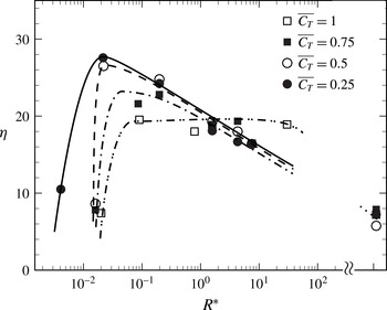
Figure 22. Figure showing the variation of propulsive efficiency (
 $\unicode[STIX]{x1D702}$
) with
$\unicode[STIX]{x1D702}$
) with
 $R^{\ast }$
at constant thrust coefficient (
$R^{\ast }$
at constant thrust coefficient (
 $\overline{C_{T}}$
). The same
$\overline{C_{T}}$
). The same
 $\overline{C_{T}}$
is achieved by choosing an appropriate value of the reduced frequency (
$\overline{C_{T}}$
is achieved by choosing an appropriate value of the reduced frequency (
 $k$
), which would in general be larger for the more flexible (lower
$k$
), which would in general be larger for the more flexible (lower
 $R^{\ast }$
) cases, as suggested by figure 9(a). Data for this plot are taken from 6 flexible foil cases for which we have measurements as a function of reduced frequency (
$R^{\ast }$
) cases, as suggested by figure 9(a). Data for this plot are taken from 6 flexible foil cases for which we have measurements as a function of reduced frequency (
 $k$
), as shown in table 1. Four sets of data are shown corresponding to
$k$
), as shown in table 1. Four sets of data are shown corresponding to
 $\overline{C_{T}}$
values of 0.25, 0.5, 0.75 and 1.
$\overline{C_{T}}$
values of 0.25, 0.5, 0.75 and 1.
Although the effects of reduced frequency on the thrust and efficiency have been presented in § 4.1, most of the subsequent results presented have been at a fixed reduced frequency (
 $k\approx 6$
). On a more general note, the efficiency and thrust coefficient are functions of both
$k\approx 6$
). On a more general note, the efficiency and thrust coefficient are functions of both
 $R^{\ast }$
(or (
$R^{\ast }$
(or (
 $f/f_{n1}$
)) and
$f/f_{n1}$
)) and
 $k$
. Another important way of looking at the results to see the effect of flexibility directly would be to look at the variation of propulsive efficiency as a function of
$k$
. Another important way of looking at the results to see the effect of flexibility directly would be to look at the variation of propulsive efficiency as a function of
 $R^{\ast }$
, while maintaining the thrust coefficient (
$R^{\ast }$
, while maintaining the thrust coefficient (
 $\overline{C_{T}}$
) to be the same. In this case, the same
$\overline{C_{T}}$
) to be the same. In this case, the same
 $\overline{C_{T}}$
can be achieved by choosing an appropriate value of the reduced frequency (
$\overline{C_{T}}$
can be achieved by choosing an appropriate value of the reduced frequency (
 $k$
), which would in general be larger for the more flexible (lower
$k$
), which would in general be larger for the more flexible (lower
 $R^{\ast }$
) cases, as suggested by figure 9(a). We have used for this figure data from the two flexible flap cases shown in figure 9 and an additional 4 cases for which we have data as a function of reduced frequency (
$R^{\ast }$
) cases, as suggested by figure 9(a). We have used for this figure data from the two flexible flap cases shown in figure 9 and an additional 4 cases for which we have data as a function of reduced frequency (
 $k$
) as shown in table 1. As may be seen from figure 22, at a given
$k$
) as shown in table 1. As may be seen from figure 22, at a given
 $\overline{C_{T}}$
, there exists an optimal
$\overline{C_{T}}$
, there exists an optimal
 $R^{\ast }$
at which the efficiency peaks, with both the peak efficiency value and the corresponding
$R^{\ast }$
at which the efficiency peaks, with both the peak efficiency value and the corresponding
 $R^{\ast }$
being dependent on the value of
$R^{\ast }$
being dependent on the value of
 $\overline{C_{T}}$
. At
$\overline{C_{T}}$
. At
 $\overline{C_{T}}$
of 0.25, the peak efficiency occurs at
$\overline{C_{T}}$
of 0.25, the peak efficiency occurs at
 $R^{\ast }\approx 0.02$
, similar to the peak efficiency
$R^{\ast }\approx 0.02$
, similar to the peak efficiency
 $R^{\ast }$
at a fixed
$R^{\ast }$
at a fixed
 $k$
of about 6. As
$k$
of about 6. As
 $\overline{C_{T}}$
is increased from 0.25 to 0.75, the peak efficiency values are found to drop with a shift of the corresponding
$\overline{C_{T}}$
is increased from 0.25 to 0.75, the peak efficiency values are found to drop with a shift of the corresponding
 $R^{\ast }$
to higher values. At
$R^{\ast }$
to higher values. At
 $\overline{C_{T}}=1.0$
, we find that the efficiency peak occurs over a broad range of
$\overline{C_{T}}=1.0$
, we find that the efficiency peak occurs over a broad range of
 $R^{\ast }$
values ranging from 0.1 to 30. These results show that there is in general an optimal value of
$R^{\ast }$
values ranging from 0.1 to 30. These results show that there is in general an optimal value of
 $R^{\ast }$
where the peak efficiency occurs, although this value depends on the choice of
$R^{\ast }$
where the peak efficiency occurs, although this value depends on the choice of
 $\overline{C_{T}}$
. Overall, it is clear that the efficiency and
$\overline{C_{T}}$
. Overall, it is clear that the efficiency and
 $\overline{C_{T}}$
are dependent on
$\overline{C_{T}}$
are dependent on
 $R^{\ast }$
and
$R^{\ast }$
and
 $k$
, and we will in general get an optimal
$k$
, and we will in general get an optimal
 $R^{\ast }$
for maximizing efficiency, whose value will depend on whether we choose to keep
$R^{\ast }$
for maximizing efficiency, whose value will depend on whether we choose to keep
 $\overline{C_{T}}$
or
$\overline{C_{T}}$
or
 $k$
constant, and the value of that constant.
$k$
constant, and the value of that constant.
7 Conclusions
In the present study, we experimentally investigate thrust production from a pitching flexible foil in a uniform flow. The flexible foils studied comprise a rigid NACA 0012 foil in the front (chord length
 $c_{R}$
) with a flexible flap of length
$c_{R}$
) with a flexible flap of length
 $c_{F}$
and flexural rigidity
$c_{F}$
and flexural rigidity
 $EI$
attached to its trailing edge. We investigate thrust generation for a range of flexural rigidities (
$EI$
attached to its trailing edge. We investigate thrust generation for a range of flexural rigidities (
 $EI$
) and flap length to total chord ratio (
$EI$
) and flap length to total chord ratio (
 $c_{F}/c=c_{F}/(c_{F}+c_{R})$
); the former being varied over 4 orders in magnitude and the later varied from 0 to approximately 0.7. The mean thrust generated (
$c_{F}/c=c_{F}/(c_{F}+c_{R})$
); the former being varied over 4 orders in magnitude and the later varied from 0 to approximately 0.7. The mean thrust generated (
 $\overline{C_{T}}$
) and the efficiency (
$\overline{C_{T}}$
) and the efficiency (
 $\unicode[STIX]{x1D702}$
) of thrust generation are both obtained experimentally from force and moment measurements using a load cell. In the rigid foil case, as expected, we find that the thrust generated is primarily due to the normal force on the foil (
$\unicode[STIX]{x1D702}$
) of thrust generation are both obtained experimentally from force and moment measurements using a load cell. In the rigid foil case, as expected, we find that the thrust generated is primarily due to the normal force on the foil (
 $\overline{C_{TN}}$
), with the chordwise or axial thrust contribution (
$\overline{C_{TN}}$
), with the chordwise or axial thrust contribution (
 $\overline{C_{TA}}$
) being small and negative.
$\overline{C_{TA}}$
) being small and negative.
In the flexible foil cases, there are two additional parameters, the flexural rigidity (
 $EI$
) of the flexible flap represented by a non-dimensional rigidity parameter,
$EI$
) of the flexible flap represented by a non-dimensional rigidity parameter,
 $R^{\ast }=EI/(0.5\unicode[STIX]{x1D70C}U^{2}c_{F}^{3})$
, and the ratio of flexible flap length to total chord of the foil (
$R^{\ast }=EI/(0.5\unicode[STIX]{x1D70C}U^{2}c_{F}^{3})$
, and the ratio of flexible flap length to total chord of the foil (
 $c_{F}/c$
), both of whose effects have been studied. We find that the thrust and efficiency values obtained from independent
$c_{F}/c$
), both of whose effects have been studied. We find that the thrust and efficiency values obtained from independent
 $EI$
and
$EI$
and
 $c_{F}/c$
studies collapse well when plotted against the non-dimensional rigidity parameter,
$c_{F}/c$
studies collapse well when plotted against the non-dimensional rigidity parameter,
 $R^{\ast }$
, for the range of
$R^{\ast }$
, for the range of
 $c_{F}/c$
values studied here, as shown in figure 16. The collapse is shown for data at fixed reduced frequencies (
$c_{F}/c$
values studied here, as shown in figure 16. The collapse is shown for data at fixed reduced frequencies (
 $k=\unicode[STIX]{x03C0}fc/U$
) of 3, 6 and 11. It should be noted that this parameter
$k=\unicode[STIX]{x03C0}fc/U$
) of 3, 6 and 11. It should be noted that this parameter
 $R^{\ast }$
is related to the ratio of the actual foil oscillation frequency to the first natural frequency of the flap (
$R^{\ast }$
is related to the ratio of the actual foil oscillation frequency to the first natural frequency of the flap (
 $f/f_{n1}$
). At
$f/f_{n1}$
). At
 $k\approx 6$
, we find that the peak efficiency occurs at
$k\approx 6$
, we find that the peak efficiency occurs at
 $R^{\ast }$
of approximately 0.01 and corresponds to an efficiency enhancement of approximately 300 % compared to that of the rigid foil efficiency (figure 14
b). Further, we find that the peak thrust occurs at a different
$R^{\ast }$
of approximately 0.01 and corresponds to an efficiency enhancement of approximately 300 % compared to that of the rigid foil efficiency (figure 14
b). Further, we find that the peak thrust occurs at a different
 $R^{\ast }$
value of approximately 8 and corresponds to a thrust enhancement of approximately 100 % compared to that of the rigid foil at the same
$R^{\ast }$
value of approximately 8 and corresponds to a thrust enhancement of approximately 100 % compared to that of the rigid foil at the same
 $k$
(figure 14
a), with this condition being close to the location of the resonant (
$k$
(figure 14
a), with this condition being close to the location of the resonant (
 $f/f_{n1}=1$
) condition.
$f/f_{n1}=1$
) condition.
Corresponding to these two optimal flexural rigidity parameter values, we find two distinct flap mode shapes; the peak thrust corresponding to a mode 1 type simple bending of the flap, while the peak efficiency deflection profile is distinctly different with the presence of an inflection point along the flap, which is different from the still water second mode shape of the flap. At both these optimal flexibilities, we find that it is the axial contribution to thrust that dominates, with almost the complete thrust coming from the axial contribution in the peak thrust case. Within the set of PIV measurements that we have, we find that the high thrust case coefficient corresponds to both large values of vortex circulation (
 $\unicode[STIX]{x1D6E4}/(Uc)\approx 2$
) and large lateral spacing of the vortices (
$\unicode[STIX]{x1D6E4}/(Uc)\approx 2$
) and large lateral spacing of the vortices (
 $b$
), with the latter implying a large wake Strouhal number (
$b$
), with the latter implying a large wake Strouhal number (
 $St_{w}=fb/U\approx 0.55$
). In contrast, the high efficiency case is found to correspond to relatively weaker vortices (
$St_{w}=fb/U\approx 0.55$
). In contrast, the high efficiency case is found to correspond to relatively weaker vortices (
 $\unicode[STIX]{x1D6E4}/(Uc)\approx 0.5$
) with smaller lateral spacing and therefore a smaller
$\unicode[STIX]{x1D6E4}/(Uc)\approx 0.5$
) with smaller lateral spacing and therefore a smaller
 $St_{w}$
of 0.35, which is consistent with the range of Strouhal numbers (0.20–0.40) suggested by the experiments of Anderson et al. (Reference Anderson, Streitlien, Barrett and Triantafyllou1998) for high propulsive efficiency of a foil in combined pitch and heave.
$St_{w}$
of 0.35, which is consistent with the range of Strouhal numbers (0.20–0.40) suggested by the experiments of Anderson et al. (Reference Anderson, Streitlien, Barrett and Triantafyllou1998) for high propulsive efficiency of a foil in combined pitch and heave.
Acknowledgement
This research was supported and funded by Naval Research Board, Government of India.


