INTRODUCTION
The neon flying squid (Ommastrephes bartramii) is an important oceanic cephalopod widely distributed in subtropical and temperate waters of the world (Roper et al., Reference Roper, Sweeney and Nauen1984; Bower & Ichii, Reference Bower and Ichii2005; Chen et al., Reference Chen, Qian and Liu2008b), and it is also one of the most important fisheries resources for Chinese squid jiggers (Wang & Chen, Reference Wang and Chen2005; Chen et al., Reference Chen, Qian and Liu2008b). Ommastrephes bartramii supports a major fishery in the north-west Pacific Ocean which may be separated into four stocks (Bower & Ichii, Reference Bower and Ichii2005). For the four stocks, the western winter-spring cohort of neon flying squid becomes a traditional fishing target for the Chinese squid-jigging fleet in the waters of 150°E–165°E (Wang & Chen, Reference Wang and Chen2005). During the 1980s, approximately 400,000–600,000t of this species were caught annually by the high seas squid driftnet fisheries of Japan, Korea and Taiwan, mainly around the subarctic boundary of the central North Pacific (Yatsu et al., Reference Yatsu, Midorikawa and Shimada1997; Ichii et al., Reference Ichii, Mahapatra and Okamura2006). Since 1993, Chinese squid-jigging boats have mainly operated in the waters of 38°N–42°N and 145°E–175°E (Chen et al., Reference Chen, Qian and Liu2008b).
Various methods have been used to assess this fast-growing species' population dynamics (e.g. Pierce & Guerra, Reference Pierce and Guerra1994; Yatsu et al., Reference Yatsu, Midorikawa and Shimada1997; Young et al., Reference Young, Pierce and Daly2004; Houghton et al., Reference Houghton, Doyle, Davenport and Hays2006; Ichii et al., Reference Ichii, Mahapatra and Okamura2006; Chen et al., Reference Chen, Chen and Tian2008a). The growth of this species has been studied using consecutive series of length-frequency distributions (Welch & Morris, Reference Welch and Morris1993; Yatsu et al., Reference Yatsu, Midorikawa and Shimada1997); the annual biomass of autumn cohort O. bartramii has been estimated based on catch data from the driftnet fishery (Ichii et al., Reference Ichii, Mahapatra and Okamura2006); depletion methods were successfully applied in the stock assessments of O. bartramii (Chen et al., Reference Chen, Chen and Tian2008a). Assessing cephalopod stocks is always difficult due to specific life history traits (short life cycle, high inter-individual variation of body size and weight and high inter-annual variation of abundance) (Jackson & Choat, Reference Jackson and Choat1992; Yatsu et al., Reference Yatsu, Midorikawa and Shimada1997; Quinn & Deriso, Reference Quinn and Deriso1999). Although many forms of stock assessment method have been applied for this species, there is little information on the application of the delay-difference model for the stock assessment of O. bartramii in the north-west Pacific Ocean. A continuous time delay-difference type model (CD-DM) has not been applied in this O. bartramii stock.
The Schnute–Deriso delay-difference models (D-DM) are considered to be a theoretical bridge between simple surplus-production models (SPM) and fully age-structured models (ASM) (Hilborn & Walters, Reference Hilborn and Walters1992; Quinn & Deriso, Reference Quinn and Deriso1999). This bridge was proposed by Deriso (Reference Deriso1980) and then modified by Walters & Martell (Reference Walters and Martell2004). The delay-difference models are biologically more realistic than the SP models and demand less data than the ASM. In fully ASM, detailed biological information is required, but surplus-production models (SPM) only provide an overview because of the lack of biological realism (Deriso, Reference Deriso1980; Hilborn & Walters, Reference Hilborn and Walters1992; Quinn & Deriso, Reference Quinn and Deriso1999). The discrete-time D-D model has already been applied to fishes with long life cycles (Pallare & Restrepo, Reference Pallare and Restrepo2003; Jensen et al., Reference Jensen, Gilroy and Hogan2009), shark-like fishes (Musick et al., Reference Musick, Bonfil and Stevens2005), lobster (Hall, Reference Hall1997), prawn (Dichmont et al., Reference Dichmont, Punt and Deng2003) and Moroccan octopus (Robert et al., Reference Robert, Faraj and McAllister2010). However, the traditional discrete-time formulation does not work well for populations that exhibit continuous reproduction over time (Walters & Martell, Reference Walters and Martell2004; Musick et al., Reference Musick, Bonfil and Stevens2005). Such dynamics characterize some commercially important stocks, such as shrimp and O. bartrami (Quinn & Deriso, Reference Quinn and Deriso1999; Walters & Martell, Reference Walters and Martell2004; Musick et al., Reference Musick, Bonfil and Stevens2005).
Such species, with recruitment, growth and mortality rates varying continuously over time, may be better analysed by a continuous delay-difference model. In 2011, Walters proposed a new continuous time delay-difference model (CD-DM), in which recruitment, growth and mortality rates are treated varying continuously over time (Walters, Reference Walters2011). The continuous time delay-difference model (CD-DM) provides an extremely compact assessment of the exact dynamics of total numbers and biomass for populations which continuously reproduce over time (Walters & Martell, Reference Walters and Martell2004; Walters, Reference Walters2011). Thus, we apply a continuous time delay-difference type model that may provide an alternative method for assessing O. bartramii fisheries. The delay-difference equation is a biomass dynamic model, but with biologically meaningful (directly measurable) parameters and accounting for basic time delays due to growth and recruitment (Hilborn & Walters, Reference Hilborn and Walters1992). The continuous time delay-difference model (CD-DM) provides satisfactory performance for the dynamics of processes (both reproduction and production) (Walters & Martell, Reference Walters and Martell2004). The ability to calculate reference points without need of a full age-structured data makes CD-DM an attractive option for data-poor fisheries (Walters & Martell, Reference Walters and Martell2004; Walters, Reference Walters2011). Being a bridge between ASPM (age structured production model) and SPM (surplus production model), CD-DM is an alternative model necessary for the appropriate stock assessment of O. bartramii.
In this study, a continuous time delay-difference model (CD-DM) was applied to assess the O. bartramii stock in the north-west Pacific Ocean during 2001–2004. By using it, we hope to provide an alternative approach in the stock assessment of O. bartramii. We estimated the growth and recruitment of O. bartramii on the basis of the CD-DM, and biological reference points (BRPs) and accuracy of estimates were also discussed in this work. The effects of different natural mortality rates and uncertainty on growth parameters were considered in this model. We apply a continuous time delay-difference type model that may provide an alternative method for assessing O. bartramii fisheries and bridge the gap between simple surplus production models and complex fully age-structured models. The estimated results were analysed to verify the proposed methodology and provide reference information for the sustainable management of the data-poor fisheries.
MATERIALS AND METHODS
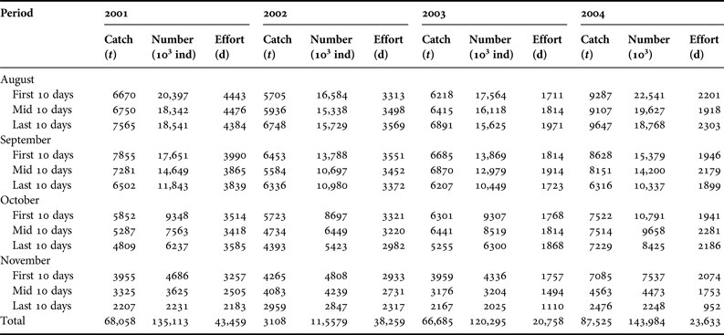
Total catch and the standardized CPUE data were collected for the winter-spring cohort of O. bartramii stock in the north-west Pacific Ocean (38°N–42°N and 150°E–165°E) during 2001–2004 (From Chen et al., Reference Chen, Qian and Liu2008b; Cao et al., Reference Cao, Chen and Chen2011). The growth rates were estimated in Yatsu et al. (Reference Yatsu, Midorikawa and Shimada1997) using statolith rings. The growth rate (mm day−1) for each individual was assessed from the mantle length at age (Yatsu et al., Reference Yatsu, Midorikawa and Shimada1997; Ichii et al., Reference Ichii, Mahapatra and Okamura2006), and generally ranged from 1.1 to 2.1 mm day−1 for males and from 1.1 to 2.5 mm day−1 for females (Yatsu et al., Reference Yatsu, Midorikawa and Shimada1997; Ichii et al., Reference Ichii, Mahapatra and Okamura2006). The Chinese squid-jigging fishery statistics during 2001–2004 are shown in Table 1.
Table 1. The Chinese squid-jigging fisheries catch and effort data of neon flying squid (Ommastrephes bartramii) from 2001 to 2004 compiled by 10-day periods (data from Chinese squid-jigging boats, from Chen et al., Reference Chen, Qian and Liu2008b and Cao et al., Reference Cao, Chen and Chen2011).
Fox surplus production model
Fox surplus production models are among the major academic models in assessment and management of modern fishery resources due to their simplicity and relatively undemanding data needs (Hilborn & Walters, Reference Hilborn and Walters1992; Su & Liu, Reference Su and Liu1998), the equation being:
 $$\eqalign{\displaystyle{{{U_{t + 1}}} \over {{U_t}}} - 1 & = r\ln \left( {\displaystyle{{q{B_\infty}} \over {{U_t}}}} \right) - q{\,f_t};\,\,{\rm MSY} = r{B_\infty} {e^{ - 1}};\,\,{\,f_{{\rm msy}}} \cr & = r/q}$$
where U t is the catch per unit effort or abundance index in year t, f is the effort, B ∞ is carrying capacity, r is intrinsic growth rate and q is catchability.
Continuous time delay-difference model
In a continuous time delay-difference model (CD-DM), the mean body weight of O. bartramii follows a relationship with age t ≥ k that leads to the Ford–Brody version of the growth model (Hilborn & Walters, Reference Hilborn and Walters1992). The model assumes that: (i) body weight growth can be approximated by the Ford–Brody model for weight at age a; (ii) fishing mortality rate is independent of age for fish aged a ≥ k; (iii) Natural mortality rate is constant for fish aged a ≥ k.
where s t is the overall survival for year t, a is age, k is the recruitment age, w a is body weight at age a, and δ and ρ are parameters. The stock-recruitment relationships (SRR) suggested by Schnute (Reference Schnute1985) and Fournier (Reference Fournier1987) have three parameters. Schnute (Reference Schnute1985) proposed that the point estimates of δ, ρ and mean body weight at age k were obtained from the von Bertalanffy growth model. Hilborn & Walters (Reference Hilborn and Walters1992) suggested the Beverton–Holt SRR models to explain the relationship between spawning biomass and recruitment, the delay-difference model (D-DM) was expressed as follows:
 $${B_t} = \left[ {\sum\limits_{a = k + 1}^\infty {{N_{a,t}}{w_a}}} \right] + {w_k}{R_t}$$
where α and β are the parameters of the Beverton–Holt SRR model, B t is the stock biomass for year t, and R t recruitment for the year t in the Beverton–Holt SRR model, and N a,t is stock number, N a,t = s t−1 N a−1,t−1. The discrete-time formulation of D-DM results in simple predictions of equilibrium biomass and numbers and continuous time delay-difference models (CD-DM) are better for recruitment, growth and mortality rates all varying continuously over time (Musick et al., Reference Musick, Bonfil and Stevens2005; Walters, Reference Walters2011). The continuous time delay-difference models (CD-DM) are expressed as follows:
 $$B(t) = \int\limits_{a = k}^\infty {N(a,t)w(a,t)da} $$
where K and W ∞ are von Bertalanffy growth coefficients and asymptotic weight, respectively. The total instantaneous mortality rate Z(t) = F(t) + M, assumed to vary over time with changes in fishing mortality rate F(t), and the biomass B ∞ and the recruitment R ∞ are the asymptotic values. The biomass equations include three parts: (i) the weight of newly added recruitment is w(k)R(t); (ii) kW ∞ N(t), basically representing the effect of food consumption on growth rate where the weight growth model in essence assumes that feeding rate per individual fish in N(t) is independent of body weight; (iii) −(Z(t) + k)B(t), represents biomass loss to all causes of loss, including instantaneous body mass metabolic loss represented by k (Walters, Reference Walters2011). The Beverton–Holt SRR model has been used to explain the relationship between spawning biomass and recruitment. (i) Given that the recruitment R(t) and fishing mortality rate F(t) are constant conditions, and C ∞ =FB ∞ , and N ∞ = R/Z, B ∞ = BPR*R (where BPR is biomass per recruit). Then, we obtain,
(ii) Given that the recruitment R(t) and fishing mortality rate F(t) can be treated as piece-wise constant over short time intervals Δt. Then, N (t + Δt) is the exact prediction of population numbers at the end of each interval given starting values, C is catch in numbers and Y is yield over the interval (t, t + Δt). The solutions (analytical solutions) of continuous time delay-difference models (CD-DM) are obtained as follow:
 $$\eqalign{B(t\, + \,\Delta t) & = {\rm} {B_\infty} \, + \,{w_\infty} \left[ {N(t) - {\rm} {N_\infty}} \right]{{\rm e}^{ - Z}}^{\Delta t} \, \cr & \quad + \,\left\{ {B(t) - {\rm} {B_\infty} - {\rm} {w_\infty} \left[ {N(t) - {N_\infty}} \right]} \right\}{{\rm e}^{ - (Z + \kappa ){\rm} \Delta t}}} $$
 $$\eqalign{ Y & = F{B_\infty} \Delta {\rm t} + F{w_\infty} [N(t) - {N_\infty} ]({\rm 1} - {\rm e}^{- Z\Delta {\rm t}} )/Z + F\{ B(t) \cr & \quad {\rm} - {B_\infty} - {w_\infty} [N(t) - {N_\infty} ]\} ({\rm 1} - {{\rm e}^{ - (Z + \kappa)\Delta t}}){\rm} /{\rm} (Z + \kappa )} $$
where B ∞ and N ∞ are the asymptotic values, H* and s* are transitional parameters, while ρ* and α* do not change except in cases where the growth curve varies over time.
Method of parameters estimation
To estimate the parameters α and β in the Beverton-Holt SRR model and the catchability coefficient q, we should maximize the log-likelihood below as the objective function.
The observation error of CPUE was considered as a lognormal distribution and expressed as follows (where U and U^ were the observed and predicted CPUEs, respectively) (Efron & Tibshirani, Reference Efron and Tibshirani1993):
Method of the selection model
We compared the continuous time delay-difference model and Fox surplus production model using Bayesian information criterion (BIC) which has the ability to incorporate the variation among models (Haddon, Reference Haddon2011), and then the smaller BIC value meant the better fit.
where m is the number of parameters to be estimated and n is the number of data points.
RESULTS
Growth parameter
The neon flying squid (O. bartramii) in the north-west Pacific Ocean during 2001–2004, attained over 500 mm mantle length (ML). The weight-at-age was converted from the BW–ML relationship, and the BW–ML relationships of female O. bartramii without geographic and size difference was BW = 0.008ML3.241, and the geographic difference was found with males, BW = 0.046ML2.901, for north-west Pacific Ocean stocks (Figure 1).
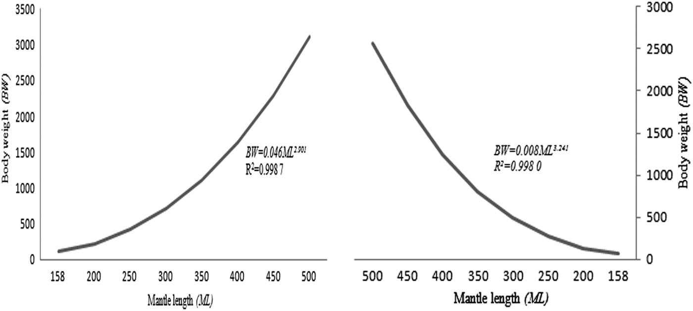
Fig. 1. Body weight (BW, g)-mantle length (ML, mm) relationship of male (left) and female (right) neon flying squid (O. bartramii) in the north-west Pacific Ocean.
The juvenile O. bartramii recruit to the fishery at a size of 150–170 mm ML. We obtained the point estimates of mean body weight at age k (W k ) by the relationship between number of increments (age) and mantle length (ML), and the BW–ML relationship. The estimated growth parameters of male and female individuals are listed in Table 2.
Table 2. Summary statistics for results of BW–ML relationships and growth rates (the individual growth rate (mm day−1) from Yatsu et al., Reference Yatsu, Midorikawa and Shimada1997 and Ichii et al., Reference Ichii, Mahapatra and Okamura2006).

Stock-recruitment relationships (SRR)
The Beverton–Holt SRR model was used to explain the relationship between spawning biomass and recruitment. The increments were assumed to be formed daily in Yatsu et al. (Reference Yatsu, Midorikawa and Shimada1997), and the growth rate was highest for individuals hatched in summer. In the continuous time delay-difference model, the mean body weight of the recruit O. bartramii follows a relationship for age t ≥ k that leads to the Ford–Brody version of the von Bertalanffy growth model. The hatchery was almost year-round, and the lifespan was likely 1 year since mature individuals were 7–10 months old. The frequency distribution of the parameters α, β and κ in the Beverton–Holt SRR model were evaluated (Figure 2).
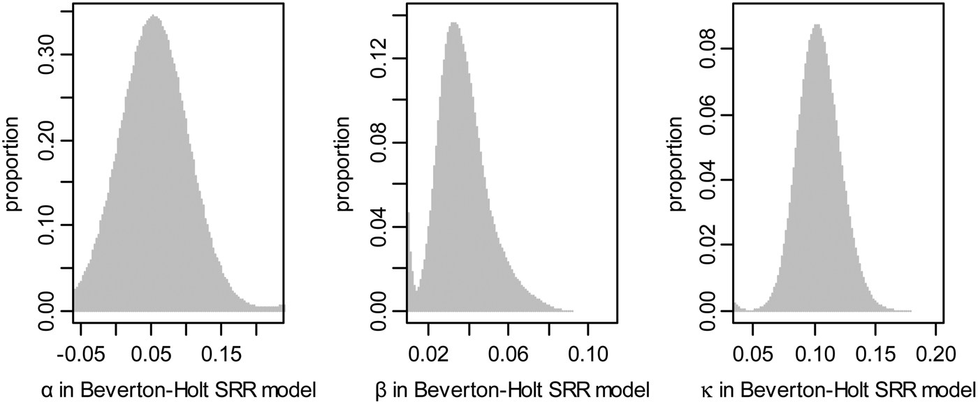
Fig. 2. Frequency distribution of the parameters α, β and κ in the Beverton–Holt SRR model.
Equilibrium spawning stock and biological reference points (BRPs)
We obtained Spawning biomass (S), Recruits (R) and harvest rate of the O. bartramii stock (2001–2004) using the median values of α, β and κ obtained. The instantaneous natural mortality M is ~0.03–0.1/10 days, from Chen et al. (Reference Chen, Qian and Liu2008b). In this study, we used the parameters M at about 0.089/10 days. The biomass (B), mean body weight (MBW) and the fishing mortality (F) of the O. bartramii stock were estimated during the fishing seasons of 2004 (Table 3).
Table 3. Biomass, mean body weight (BW) and fishing mortality (F) of the neon flying squid (O. bartramii) stock were estimated from August to November in 2004.

The maximum sustainable yield (MSY) and the fishing mortality for achieving MSY (F MSY) are still the important goals of fisheries management. Biomass dynamics models provide estimates of a number of biological reference points (BRPs): maximum sustainable yield (MSY), the fishing mortality for achieving MSY (F MSY), and the biomass (B) at MSY (B MSY). The biomass at MSY (B MSY) of the winter-spring cohort was 380,000 t–560,000 t. The population sizes ranged from 183.9 to 201.8 million squid in early September 2004. Biomass increased as harvest rate decreased, whereas recruitment peaked at an approximate harvest rate of 0.45.
Uncertainty estimator of the Beverton-Holt model's parameters
We estimated the uncertainty of parameters α, β and κ in the Beverton–Holt SRR model. Actually mean weight is expected to differ from weight at the mean length by a multiplicative factor (1 + 3.0CV2), where CV is the coefficient of variation in body length at age, typically in the range 0.05–0.15. The mean body weight at that age t is given approximately by (1 + 3.0CV2) αML3, and it is this weight that we used in estimating w(k) and w ∞ . We estimated the parameters α, β and κ in the Beverton–Holt SRR model, and the 95% confidence interval of parameter and the coefficient of variation (CV) in the continuous time delay-difference models (Table 4).
Table 4. The 95% confidence intervals of parameters in the Beverton–Holt SRR model including median values and the coefficient of variation (CV).

CD-DM compared with SPM by Bayesian information criterion (BIC)
The predicted CPUEs of the Fox surplus production model and continuous time delay-difference model were compared. For the continuous time delay-difference model (CD-DM), the annual fluctuations in CPUEs were captured more efficiently than those in the Fox surplus production model. The ability to calculate reference points without need of a full age-structured data makes the continuous time delay-difference model an attractive option for O. bartramii stock assessment. With the comparison between those two models, BIC tended to select the continuous time delay-difference model as the better model (Table 5).
Table 5. Model selection criterion (Bayesian information criterion, BIC) for the comparison of the continuous time delay-difference model and Fox surplus production model.

CD-DM compared with ASM on the predicted biomass and numbers
We constructed the Stock-Recruitment Relationships (SRR) model with very small age-time increments Δa, Δt < 0.1, and forced this model with the recruitment R(t) and F(t) varying in annual sinusoidal pattern over time. There is little detailed age-structure information about the O. bartramii stock. Thus, a simulation example was used to illustrate how the continuous time delay-difference model exactly tracks the total biomass and numbers predicted from the fully age-structured accounting model (ASM). The biomasses and numbers summed over age for the continuous time delay-difference model (CD-DM) do indeed track the simple model predictions more and more precisely as the age-time increment becomes smaller (Figure 3).
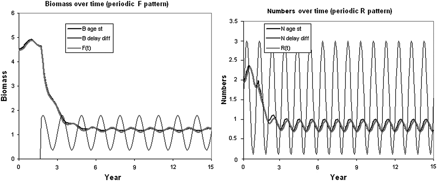
Fig. 3. An example (trajectories) of how the continuous time delay-difference (delay diff) model tracks the total biomass and numbers predicted from the age-structured (age st) model, in which F pattern over time is shown on the biomass plots, R pattern is shown on the numbers plots (modified from Walters, Reference Walters2011).
DISCUSSION
The continuous time delay-difference models (CD-DM) have not been applied in this species. The main objective of this study is to provide an alternative method for O. bartramii stock assessment. The continuous time delay-difference models (CD-DM) were modified from the discrete-time delay-difference model, in which recruitment, growth and mortality rates are treated as varying continuously over time. We used the continuous time delay-difference model (CD-DM) and obtained population sizes of 183.9–201.8 million squid during early September 2004. We evaluated the population parameters, biological reference points (BRPs) and accuracy of estimates. The effects of using a multiplicative factor were evaluated in fitting the stock-recruitment (SR) model in this study. The stock did not have a status of sustainable according to the available data, which suggests that measures should be taken for the sustainable utilization of this stock. The exploitation of the stock started in the early 1970s. Over the last two decades, Japan, South Korea and Taiwan are the main countries that have fished O. bartramii. The catches of O. bartramii in the North Pacific are less than half of those before the driftnet moratorium went into effect (Bower & Ichii, Reference Bower and Ichii2005; Ichii et al., Reference Ichii, Mahapatra and Okamura2006).
Different forms of stock assessment have been used to estimate the population dynamics of the north-west Pacific Ocean O. bartramii stock. Murata (Reference Murata1990) indicated that the initial (pre-fishing season) annual population sizes ranged from 139 to 154 million squid, using the surplus production model, in early September 1979, and Chen et al. (Reference Chen, Chen and Tian2008a) reported the initial population at about 235.4–307.1 million squid using the depletion model; Cao et al. (Reference Cao, Chen and Chen2011) used Virtual Population Analysis (VPA) to give a range of estimated MSY of the winter-spring cohort of 10,300 to 14,300 t. The importance of including explicitly the natural mortality (i.e. predation mortality) in stock assessment models had been discussed in the literature (e.g. Livingston & Methot, Reference Livingston and Methot1998; Hollowed et al., Reference Hollowed, Ianelli and Livingston2000; Jiao et al., Reference Jiao, Hayes and Cortés2009; Moustahfid et al., Reference Moustahfid, Tyrrell and Link2009; Tyrrell et al., Reference Tyrrell, Link and Moustahfid2011; Wang et al., Reference Wang, Zheng and Yu2014). Effects of using different natural mortality rates (M) were evaluated in fitting the stock-recruitment (SR) model. However, there is little information on the application of the delay-difference model for the stock assessment of O. bartramii.
The delay-difference equation is a biomass dynamic model, but with biologically meaningful (directly measurable) parameters and accounting for basic time delays due to growth and recruitment (Hilborn & Walters, Reference Hilborn and Walters1992). This model has been successfully used to estimate stock size in shark-like fish (Musick et al., Reference Musick, Bonfil and Stevens2005), fish with long life cycles (Pallare & Restrepo, Reference Pallare and Restrepo2003; Jensen et al., Reference Jensen, Gilroy and Hogan2009), lobster (Hall, Reference Hall1997), prawn (Dichmont et al., Reference Dichmont, Punt and Deng2003) and Moroccan octopus (Robert et al., Reference Robert, Faraj and McAllister2010). The commercially important fish stocks, such as O. bartramii, could been more accurately assessed with the continuous time delay-difference type model (CD-DM) due to recruitment, growth, and mortality rates all varying continuously over time (Su & Liu, Reference Su and Liu1998; Walters & Martell, Reference Walters and Martell2004; Musick et al., Reference Musick, Bonfil and Stevens2005; Walters, Reference Walters2011). Because the discrete-time delay-difference model does not perform well for species which continuously reproduce over time (Deriso, Reference Deriso1980; Musick et al., Reference Musick, Bonfil and Stevens2005), in 2011, Walters proposed the new continuous time delay-difference model, in which recruitment, growth and mortality rates are treated as varying continuously over time. Thus, we apply a continuous time delay-difference type model that may provide an alternative method for assessing O. bartramii fisheries. The mantle length–weight relationship could be used to explain the effect of variations in survival rate on mean body weight and to estimate the survival rate for a particular observed mean body weight (Walters, Reference Walters2011; Su & Randall, Reference Su and Randall2012). The growth rates were estimated using statolith rings (Yatsu et al., Reference Yatsu, Midorikawa and Shimada1997), the mantle length–age relationships were linear, and slope and intercept values differed by geographic area, hatch season and sex (Yatsu et al., Reference Yatsu, Midorikawa and Shimada1997). The continuous time delay-difference model (CD-DM) provides an extremely efficient assessment of the exact dynamics of total numbers and biomass for populations which continuously reproduce over time (Musick et al., Reference Musick, Bonfil and Stevens2005; Walters, Reference Walters2011).
In summary, a continuous time delay-difference model (CD-DM) was applied to assess the O. bartramii stock in the north-west Pacific Ocean during 2001–2004. By using it, we hope to provide an alternative approach in the stock assessment of neon flying squid and filled the gaps in simple surplus production models and complex fully age-structured models. By comparison with the other models, the O. bartramii stock could be treated better by continuous time delay-difference model (CD-DM), and the ability to calculate reference points without need of a full age-structured data makes the CD-DM an attractive option for data-poor fisheries. The continuous time model has provided satisfactory performance for the dynamics of processes (both reproduction and production). The estimated results were analysed to verify the proposed methodology and provide reference information for the sustainable management of the neon flying squid (O. bartramii) stock. In the future, we plan to conduct further research with data from other time periods.
ACKNOWLEDGEMENTS
The authors acknowledge the constructive input from Drs Zhenming Su, Yan Jiao, Kui Zhang, two anonymous reviewers and the Associate Editor.
FINANCIAL SUPPORT
This work was supported by Fundamental Research Funds for the Central Universities of China (Grant No. 201022001) and Funds for Shandong Province Education Science Twelfth Five-Year Guideline Project (Grant No. 2011GG378).

