


1. Introduction
The interaction of a rotor with turbulent flow can generate noise known as turbulence-ingestion noise, which is a significant concern for the design of marine propellers as well as many devices in aeronautical, automotive and wind energy applications. The inflow turbulence, often resulting from the wakes of upstream bodies such as stators, grilles and control surfaces, is highly complex and distorted as it is ingested into the rotor. The wide range of spatial and temporal scales present in the flow causes broadband rotor acoustic response. Tonal noise can be produced by the periodic passing of rotor blades through coherent turbulence structures and presence of a Kármán vortex street in the wake. In addition, self-noise is generated through the rotor's viscous interaction with the flow, as a result of boundary-layer eddies convected past the blade trailing edge, flow separation and vortex shedding (Blake Reference Blake2017).
Historically, turbulence-ingestion noise is modelled in the framework of gust-response theory for a thin, flat-plate airfoil (e.g. Sears Reference Sears1941; Amiet Reference Amiet1975, Reference Amiet1976) in conjunction with the strip-theory approximation. Each rotor blade is treated as a series of airfoils along the blade span in translation at the local relative velocity, and a linear, inviscid flow theory is employed to estimate the unsteady loading on the airfoil. The radiated acoustic field is calculated by solving a wave equation with the blade unsteady loading as the source term, often using the integral form of the Ffowcs Williams–Hawkings (FW–H) equation (Ffowcs Williams & Hawkings Reference Ffowcs Williams and Hawkings1969). The classical unsteady thin-airfoil theory of Sears (Reference Sears1941) is based on the assumption of solenoidal gust velocity and applicable only to dipole radiation from acoustically compact airfoils. If the airfoil (blade) chord is acoustically non-compact, compressibility effects become important. Theories accounting for acoustic scattering by the airfoil leading and trailing edges have been developed by, for example, Amiet (Reference Amiet1975), Howe (Reference Howe2001) and Roger & Moreau (Reference Roger and Moreau2005). Further generalizations have been made to incorporate the effects of airfoil thickness, shape and induced turbulence distortions (e.g. Gershfeld Reference Gershfeld2004; Moreau, Roger & Jurdic Reference Moreau, Roger and Jurdic2005; Santana et al. Reference Santana, Christophe, Schram and Desmet2016; Zhong et al. Reference Zhong, Zhang, Peng and Huang2020). For application to rotor noise, however, the aforementioned analytical approaches cannot accurately account for the effects of the real three-dimensional geometry of the rotor and the aerodynamic interaction among blades. Furthermore, these methods rely on empirical models for the wavenumber spectra and correlation length scales of the incoming turbulence, which is typically assumed homogeneous and isotropic (e.g. Mani Reference Mani1971; Homicz & George Reference Homicz and George1974), and thus highly simplified relative to realistic turbulent gusts.
Early experimental investigations of turbulence-ingestion noise also involved homogeneous and isotropic turbulent inflows (e.g. Sevik Reference Sevik1974; Wojno, Muller & Blake Reference Wojno, Muller and Blake2002a,Reference Wojno, Muller and Blakeb). Sevik (Reference Sevik1974) performed a pioneering experiment of a rotor in grid-generated turbulence in a water tunnel. The rotor had 10 blades with a constant chord length of 1 inch and a radius-to-chord ratio of 4. The power spectral density of the unsteady thrust measured was compared with the theoretical prediction based on a two-dimensional, incompressible, thin-airfoil theory and a two-point velocity correlation model for the ingested turbulence, which was assumed homogeneous and isotropic. The theory successfully predicted the broadband component of the experimental spectra but failed to capture the spectral humps at multiples of the blade passing frequency (BPF), known as haystacking, because it did not account for the blade-to-blade correlation due to successive blades cutting the same turbulence structures. The blade-to-blade correlation of acoustic sources can be enhanced by rotor-induced turbulence distortions. As turbulent eddies, even if initially isotropic, are drawn towards a rotor, they are stretched in the axial direction and contracted in the transverse direction due to flow acceleration, and thus necessarily anisotropic. Hanson (Reference Hanson1974) found in static tests of an aircraft engine fan in atmospheric turbulence that the ratio of streamwise to transverse integral length scales for the inlet turbulence was as high as  $400\!:\!1$, resulting in noise with narrow spectral peaks at harmonics of the BPF. Such a strong distortion is, however, created by the sink-like behaviour of static inflow as pointed out by Hanson (Reference Hanson1974), and not representative of normal operating conditions. Turbulence distortions induced by a fan or propeller in forward motion are much weaker, and their role in noise generation is of significant interest.
Majumdar & Peake (Reference Majumdar and Peake1998) developed a theoretical model for the noise produced by the ingestion of atmospheric turbulence, modelled by the isotropic von Kármán spectra, into an aircraft engine fan. Rapid distortion theory was used to obtain the distorted turbulence field in the rotor plane, and the radiated sound was evaluated using the strip theory and asymptotic techniques. Their analysis showed that, consistent with the experimental result of Hanson (Reference Hanson1974), in static test conditions strong inflow contraction leads to highly elongated eddies and sharp tonal noise at BPF harmonics. Under typical flight conditions, on the other hand, the eddies are much less distorted and no haystacking tones are present, but the power level of the broadband noise component is much greater than that in the static case. Robison & Peake (Reference Robison and Peake2014) extended the analysis of Majumdar & Peake (Reference Majumdar and Peake1998) to turbulent inflows that are non-axisymmetric due to either an adjacent second rotor or a non-zero incidence angle. They found the same qualitative distortion effect on acoustics as in the axisymmetric case, i.e. high distortion (static condition) leads to strong spectral peaks at multiples of BPF whereas low distortion (flight condition) produces broadband noise only, although the spectral levels can be significantly affected by the inflow asymmetry.
Rotor interaction with realistic turbulent flows has been investigated in a number of recent experimental and theoretical studies. Catlett, Anderson & Stewart (Reference Catlett, Anderson and Stewart2012) incorporated the effect of inhomogeneity and anisotropy in their ad hoc inflow velocity-correlation model, and used it in the Sears thin-airfoil theory to predict the blade unsteady-force spectra and, treating the rotor as an acoustically compact dipole source, radiated acoustic pressure spectra. Using this model, they obtained an improved prediction of the noise from a rotor right behind the trailing edge of an airfoil compared with the prediction of an isotropic model. Glegg, Morton & Devenport (Reference Glegg, Morton and Devenport2012) and Glegg, Devenport & Alexander (Reference Glegg, Devenport and Alexander2015) developed a rotor-noise theory in the time domain which facilitated treatment of inhomogeneous turbulent inflow. Their method is based on the unsteady loading term in the FW–H equation coupled with a strip theory and a thin-airfoil theory to relate the blade-loading space–time correlations to the space–time correlations of the upwash velocity encountered by the rotor blades. The effect of turbulence distortion by the rotor inflow can be included in this method using rapid distortion theory (Glegg et al. Reference Glegg, Kawashima, Lachowski, Devenport and Alexander2013). Researchers at Virginia Tech (VT) (Alexander et al. Reference Alexander, Devenport, Morton and Glegg2013, Reference Alexander, Devenport, Wisda, Morton and Glegg2014; Alexander, Devenport & Glegg Reference Alexander, Devenport and Glegg2017; Wisda et al. Reference Wisda, Alexander, Devenport and Glegg2014, Reference Wisda, Murray, Alexander, Nelson, Devenport and Glegg2015; Murray et al. Reference Murray, Devenport, Alexander, Glegg and Wisda2018) conducted a series of experiments with a 10-bladed, modified and scaled-up Sevik rotor partially immersed in a thick flat-plate turbulent boundary layer. They measured the sound produced by the rotor over a range of operating conditions and found haystacking spectral peaks, which grew in amplitude and appeared at higher harmonics of the BPF with decreasing rotor advance ratio (increasing thrust). Four-dimensional space–time correlations of the inflow velocity were measured to provide input for the theoretical model of Glegg et al. (Reference Glegg, Devenport and Alexander2015), which gave reasonable noise predictions at low and moderate thrust. At high thrust, particle image velocimetry measurements and tuft flow visualization revealed boundary-layer separation and flow reversal in the vicinity of the rotor blade disk, and blade interaction with the vortex structures in the separation region was identified as an additional source of tonal noise (Murray et al. Reference Murray, Devenport, Alexander, Glegg and Wisda2018).
In a more recent experiment, VT researchers (Alexander et al. Reference Alexander, Molinaro, Hickling, Murray, Devenport and Glegg2016; Hickling et al. Reference Hickling, Alexander, Molinaro, Devenport and Glegg2017; Molinaro et al. Reference Molinaro, Balantrapu, Hickling, Alexander, Devenport and Glegg2017) considered the noise of a rotor ingesting the wake of a circular cylinder. The same modified Sevik rotor as used in their previous rotor-boundary layer interaction experiment (Alexander et al. Reference Alexander, Devenport and Glegg2017; Murray et al. Reference Murray, Devenport, Alexander, Glegg and Wisda2018) was employed. The rotor diameter is 457 mm and the hub diameter is 127 mm. The cylinder diameter  $D$ is
  $1/9$ of the rotor diameter, and the centre of the cylinder is
  $20D$ upstream of the rotor centre. The free stream velocity
  $U_{\infty }$ is fixed at
  $20\ \textrm {m}\ \textrm {s}^{-1}$. Various rotor advance ratios, wake-strike positions and yaw angles were included in the experimental test matrix. The experimental results indicate that the sound pressure level increases with decreasing rotor advance ratio and, when the advance ratio is sufficiently low, i.e. with sufficiently large thrust, haystacking peaks appear in the acoustic pressure spectra. They also show that the effect of wake-strike position is relatively small; stronger noise is generated when the wake strikes the rotor at
  $75\,\%$ of the rotor radius compared with 100 % of the radius. Increasing the yaw angle was found to increase the sound pressure level at frequencies above the BPF. Because of the rich physics and wide range of spatiotemporal scales in a relatively clean flow configuration, this experiment, like the well known rod–airfoil configuration for airfoil–wake interaction noise (Jacob et al. Reference Jacob, Boudet, Casalino and Michard2005; Giret et al. Reference Giret, Sengissen, Moreau, Sanjosé and Jouhaud2015), provides a good benchmark test case for validating computational predictions of rotor turbulence-ingestion noise.
In the present work, the baseline configuration of the VT rotor–wake experiment (Alexander et al. Reference Alexander, Molinaro, Hickling, Murray, Devenport and Glegg2016; Hickling et al. Reference Hickling, Alexander, Molinaro, Devenport and Glegg2017; Molinaro et al. Reference Molinaro, Balantrapu, Hickling, Alexander, Devenport and Glegg2017), in which the wake strikes a zero-yaw rotor at the centre, is analysed numerically. Two off-centre wake-strike positions at  $75\,\%$ and
  $100\,\%$ of the rotor radius have also been considered (Wang Reference Wang2017; Wang, Wang & Wang Reference Wang, Wang and Wang2017) but are not discussed here for brevity. The objectives are to demonstrate the predictive capability of a large-eddy simulation (LES) based computational methodology for rotor turbulence-ingestion noise and, using the detailed simulation data, investigate the acoustic source characteristics and mechanisms. Use of LES and other high-fidelity simulation techniques for rotor noise, and more generally turbomachinery noise, is relatively new. Earlier computations relied upon Euler equations or Reynolds-averaged Navier–Stokes (RANS) equations. Carolus, Schneider & Reese (Reference Carolus, Schneider and Reese2007) were perhaps the first to apply LES to an entire rotor for noise prediction. They computed the flow past a low-Mach-number ducted fan with six blades downstream of a turbulence-generating grid using an incompressible-flow finite-element solver, and employed an analytical model to predict the radiated noise. With only five million elements for the entire configuration, they obtained reasonable agreement with measurements at some frequencies but significant discrepancies were also observed. Arroyo et al. (Reference Arroyo, Leonard, Sanjose, Moreau and Duchaine2019) used wall-modelled compressible LES with 75 million unstructured-mesh cells to simulate a
  $1/5$ scale model turbofan stage in a periodic sector of
  $360^{\circ }/11$ containing two rotor blades and five stator vanes. The far-field acoustics was predicted by the FW–H equation and Goldstein's analogy. Similar rotor/stator turbofan configurations were simulated in their entirety (
 $360^{\circ }$) by Casalino, Hazir & Mann (Reference Casalino, Hazir and Mann2018) using a hybrid lattice-Boltzmann/very large-eddy simulation method and by Suzuki et al. (Reference Suzuki, Spalart, Shur, Strelets and Travin2018, Reference Suzuki, Spalart, Shur, Strelets and Travin2019) using a zonal hybrid RANS/LES method for noise predictions. The lattice-Boltzmann/very large-eddy simulation method was also employed by Moreau (Reference Moreau2019a) to simulate a ring fan in a clean inflow at a tip Mach number
  $0.15$. The sound was computed directly from the simulation and showed better agreement with measurements than the predictions using unsteady RANS and the FW–H equation. A review of turbomachinery noise modelling and computation has been provided by Moreau (Reference Moreau2019b). Note that the aforementioned computations all involved ducted fans (rotors) with complex source and propagation effects such as rotor–stator interaction, tip-leakage vortices, and strong near-field diffraction and refraction effects, which made it difficult to isolate individual acoustic source mechanisms. The VT open-rotor experiment simulated in the present work provides a cleaner configuration for a fundamental study of the characteristics and physical mechanisms of turbulence-ingestion noise with high levels of detail and accuracy.
A schematic of the flow configuration is illustrated in figure 1. Two rotor advance ratios,  $J = U_{\infty }/(n D_r) = 1.44$ and
  $1.05$, where
  $n$ is the rotational speed of the rotor in revolutions per second and
  $D_r$ is the rotor diameter, are considered. The former corresponds to a nominally zero-thrust condition whereas the latter produces a relatively low thrust. The LES is performed for the entire rotor at the experimental Reynolds number of
  $Re_{D_r} = U_{\infty } D_r/\nu = 5.83 \times 10^5$ based on the free stream velocity and the rotor diameter. The free stream Mach number is
  $M_{\infty } = U_{\infty }/c_{\infty } = 0.058$. Using the FW–H equation, the sound field is calculated and validated against experimental measurements. The dominant noise source associated with the unsteady loading on blades is investigated in detail to reveal its spatiotemporal characteristics and relation to the turbulent flow field. The distortion of the wake turbulence by the rotor is examined through an analysis of velocity two-point and space–time correlations, and the accuracy of the classical Sears theory for predicting the rotor wake-ingestion noise is evaluated using the LES data. Guided by the theory, the appropriate Mach number scaling of the acoustic spectra for different source locations and rotational speeds is identified and verified, and contributions of the mean velocity defect and turbulent fluctuations in the wake to noise generation are quantified.

Figure 1. Schematic of rotor interaction with a cylinder wake.
2. Numerical methodology
Because of the low flow Mach number, a hybrid approach combining LES based on incompressible flow equations with an aeroacoustic theory is well suited for the present study (Wang, Freund & Lele Reference Wang, Freund and Lele2006) and therefore employed. The unsteady loading on blade surfaces is computed by the LES and used to evaluate the sound pressure based on the FW–H integral formulation of the Lighthill equation (Lighthill Reference Lighthill1952; Ffowcs Williams & Hawkings Reference Ffowcs Williams and Hawkings1969).
2.1. Method for flow simulation
As observed in the experiment of Alexander et al. (Reference Alexander, Molinaro, Hickling, Murray, Devenport and Glegg2016), the presence of the rotor has a negligible effect on the generation and development of the upstream cylinder wake because of the large separation distance between the rotor and the cylinder. This allows the simulations of wake generation and wake-rotor interaction to be carried out separately. The wake-generation simulation, discussed in detail in § 3, is performed in the stationary frame of reference and provides inflow data for the rotor simulation. The latter is conducted in the rotor frame of reference in which the spatial coordinates are fixed on the rotor. This decoupled approach is computationally efficient because, aside from avoiding the need for using a sliding-mesh technique and the associated computational overhead, the cylinder wake only needs to be computed once and the same inflow data saved can be used repeatedly for rotor simulations with different rotor advance ratios and wake-strike positions.
The rotor-frame simulations are performed using the conservative formulation (Beddhu, Taylor & Whitfield Reference Beddhu, Taylor and Whitfield1996) of the spatially filtered (denoted by an overbar) Navier–Stokes equations and continuity equation,
 \begin{equation} \left. \frac{\partial\bar{u}^r_i}{\partial t} \right|_r + \frac{\partial}{\partial x_j^r} \bar{u}^r_i \bar{u}^r_j - \frac{\partial}{\partial x_m^r} \epsilon_{mjk} \varOmega_j x_k^r \bar{u}^r_i + \epsilon_{ijk} \varOmega_j \bar{u}^r_k = - \frac{1}{\rho} \frac{\partial\bar{p}}{\partial x_i^r} + \nu \frac{\partial^2 \bar{u}^r_i}{\partial x_j^r \partial x_j^r} + \frac{\partial}{\partial x_j^r} \tau_{ij}^r, \end{equation}
 \begin{equation} \frac{\partial\bar{u}^r_i}{\partial x_i^r} = 0, \end{equation}
where  $\bar {u}^r_i$ are components of the absolute velocity in the rotating frame of reference
  $x^r_i$,
  $\varOmega _i$ are components of the angular velocity of the reference frame,
  $p$ and
  $\rho$ are the fluid pressure and density, respectively,
  $\nu$ is the kinematic viscosity,
  $\epsilon _{ijk}$ is the alternating tensor,
  $\tau _{ij}^r = \bar {u}^r_i\bar {u}^r_j-\overline {u_i^r u_j^r}$ is the subgrid-scale stress, and
  ${\partial }/{\partial {t}}|_r$ is the time derivative with respect to the rotating frame of reference. The equations solved in the stationary frame of reference are those in (2.1) and (2.2) with
  $\varOmega _j$ set to zero and the superscript and subscript ‘
 $r$’ dropped.
A finite volume, unstructured-mesh LES code for incompressible flow developed at Stanford University (You, Ham & Moin Reference You, Ham and Moin2008) is enhanced with the rotating-frame formulation (2.1) and used for flow simulations. It employs a fully implicit, fractional-step time-advancement method and an algebraic multigrid Poisson solver for pressure, and is second-order accurate in both time and space. The spatial discretization is energy conserving and low dissipative, and thus can accurately capture a wide range of flow scales relevant to sound generation. The effect of subgrid-scale motions is modelled using the dynamic Smagorinsky model (Germano et al. Reference Germano, Piomelli, Moin and Cabot1991). The accuracy of this code for flow-noise studies has been established in a number of previous configurations including rough-wall boundary layers (Yang & Wang Reference Yang and Wang2013), tandem cylinders and airfoil in a cylinder wake (Eltaweel et al. Reference Eltaweel, Wang, Kim, Thomas and Kozlov2014).
2.2. Method for acoustic calculation
The FW–H integral formulation of the Lighthill equation, which allows surfaces in arbitrary motion (Ffowcs Williams & Hawkings Reference Ffowcs Williams and Hawkings1969; Goldstein Reference Goldstein1976) is employed,
 \begin{align} p({\boldsymbol{x}},t) = \iint_{S(\tau)}n_jp_{ij}\frac{\partial{G}}{\partial{y_i}}\,\mathrm{d}S\,\mathrm{d}\tau-\iint_{S(\tau)}\rho_{\infty} n_j V_j \frac{\partial{G}}{\partial{\tau}}\,\mathrm{d}S\,\mathrm{d}\tau+\iint_{V(\tau)}T_{ij}\frac{\partial^2{G}}{\partial{y_i}\partial{y_j}}\,\mathrm{d}V\,\mathrm{d}\tau, \end{align}
where  $p({\boldsymbol {x}},t)$ is the fluctuating pressure, which is equal to the acoustic pressure outside the nonlinear flow region, at observer location
  ${\boldsymbol {x}}$ and observer time
  $t$;
$t$;  $S(\tau )$ is the integration surface, taken to be the solid surface, at source emission time
  $\tau$;
  $n_j$ are components of the unit normal to
  $S$ pointing into the fluid;
  $p_{ij}$ is the compressive stress tensor dominated by pressure;
  $G = G({\boldsymbol {x}}, t; {\boldsymbol {y}}, \tau )$ is the free-space Green's function;
  ${\boldsymbol {y}}$ is the source position vector with
  $y_i$ being its components;
  $\rho _{\infty }$ is the ambient density;
  $V_j$ are components of the surface velocity; and
  $T_{ij}$ is the Lighthill stress tensor dominated by
  $\rho _{\infty } u_i u_j$ and distributed in the source region
  $V(\tau )$. The three terms on the right-hand side represent loading noise, thickness noise and quadrupole contributions, respectively. At low Mach numbers unsteady loading is the dominant source of noise. As a result, (2.3) can be simplified in the acoustic far-field as (Brentner & Farassat Reference Brentner and Farassat2003)
 \begin{equation} p({\boldsymbol{x}},t) \approx \frac{1}{4{\rm \pi} c_{\infty}}\frac{\partial}{\partial t}\int_S \left[\frac{r_{d_i}}{r_d^2}\frac{p_{ij}n_j}{|1-M_r|}\right]_{\tau^{\ast}}\,\mathrm{d}S, \end{equation}
where  $r_d=|{\boldsymbol {x}}-{\boldsymbol {y}}(\tau )|$ is the distance between the observer and the source,
  $r_{d_i} = x_i-y_i$, and
  $M_r = (r_{d_i}/r_d)M_i$ is the Mach number of the source in the radiation direction with
  $M_i$ being components of the source Mach number vector. The integrand is evaluated at the retarded time
  $\tau ^{\ast }$ which is the root of the equation
  $\tau = t - |{\boldsymbol {x}}-{\boldsymbol {y}}(\tau )|/c_{\infty }$. For the rotor geometry and Mach numbers considered in this study, the rotor blades can be assumed acoustically compact in the chordwise direction but not necessarily in the radial direction. To facilitate evaluation of (2.4), each blade is divided into acoustically compact strips stacked in the radial direction, and the far-field sound is then the sum of contributions from all strips,
 \begin{equation} p({\boldsymbol{x}},t)\approx\frac{1}{4{\rm \pi} c_{\infty}}\frac{\partial}{\partial t}\sum_{n=1}^{N_b}\sum_{m=1}^{N_s}\left[ \frac{r_{d_i}}{r_d^2}\frac{F_i}{|1-M_r|} \right]^{m,n}_{\tau^{\ast}}, \end{equation}
where  $N_b$ is the number of blades,
  $N_s$ is the number of strips on a blade and
 \begin{equation} F^{m,n}_i = \int_{S_{mn}} p_{ij} n_j\,\mathrm{d}S \end{equation}
is the net unsteady force on each strip.
Alternatively, the time derivatives in (2.4) and (2.5) can be moved from the observer time to the source time using  ${\partial }/{\partial t} = ({1}/({1-M_r}))({\partial }/{\partial \tau })$, leading to (see, for example, Brentner & Farassat Reference Brentner and Farassat2003; Glegg & Devenport Reference Glegg and Devenport2017)
 \begin{equation} p({\boldsymbol{x}},t) \approx \frac{1}{4{\rm \pi} c_{\infty}} \int_S \left[ \frac{r_{d_i}}{r_d^2(1-M_r)^2} \left( \frac{\partial (p_{ij} n_j)}{\partial \tau}+\frac{p_{ij} n_j}{|1-M_r|}\frac{\partial M_r}{\partial \tau} \right) \right]_{\tau^{\ast}}\,\mathrm{d}S \end{equation}
and
 \begin{equation} p({\boldsymbol{x}},t)\approx\frac{1}{4{\rm \pi} c_{\infty}} \sum_{n=1}^{N_b}\sum_{m=1}^{N_s} \left[ \frac{r_{d_i}}{r_d^2(1-M_r)^2} \left( \frac{\mathrm{d} F_i}{\mathrm{d} \tau} + \frac{F_i}{|1-M_r|} \frac{\mathrm{d} M_r}{\mathrm{d} \tau} \right) \right]^{m,n}_{\tau^{\ast}} \end{equation}
in the acoustic far-field. In this formulation the acoustic dipole sources  ${\partial (p_{ij} n_j)}/{\partial \tau }$ and
  $\mathrm {d} F_i/\mathrm {d} \tau$ are revealed explicitly, and the terms proportional to
  ${\partial M_r}/{\partial \tau }$ are relatively small if the Mach number of the blade tip is small. Calculations performed with both formulations (2.5) and (2.8) have produced negligible differences in results.
3. Wake generation and validation
The turbulent wake is generated using LES of uniform flow over a circular cylinder at  $Re_D = 64\,800$. The wake-generation LES is performed in a rectangular computational box of sizes
  $28.8D$ in the streamwise direction,
  $36D$ in the cross-stream direction and
  $7.5{\rm \pi} D$ in the spanwise direction, where
  $D$ is the cylinder diameter. The distance from the inlet to the cylinder is
  $12.5D$, and velocity data are collected in a plane
  $10D$ downstream of the cylinder centre for use as inflow data in the rotor simulation. Uniform free stream velocity free of turbulence is imposed at the inlet. Stress-free conditions with zero normal velocity are used on the outer boundaries in the cross-stream direction. No-slip and no-penetration conditions are employed on the cylinder surface, and convective outflow boundary conditions are employed at the exit. Periodic boundary conditions are used in the spanwise direction. The computational mesh consists of 118 million hexahedral and prism cells with
  $960$ layers of cells distributed uniformly along the span. An O-type mesh block with
  $400$ cells in the circumferential direction is used around the cylinder. The height of the first layer of cells adjacent to the cylinder surface is between
  $0.2$ and
  $2.5$ wall units, with peak values located at
  $\theta \approx \pm 45^{\circ }$ from the front stagnation point.
A snapshot of the turbulent wake behind the cylinder is shown in figure 2 in terms of the second invariant of the velocity gradient tensor. Coherent vortex shedding and a broad range of turbulent flow structures are observed. Note that the spanwise domain size is much larger than those seen in typical LES of cylinder flows; it is more than twice the rotor diameter to ensure that the downstream rotor is fully immersed in the cylinder wake in the spanwise direction and the rotor noise prediction is not affected by the periodic boundary condition.

Figure 2. Cylinder wake visualized by isosurfaces of  $Q$-criterion at
  $Q(D/U_{\infty })^2=1.92$ coloured by the cross-stream velocity component.
Figure 3(a–d) shows profiles of the mean streamwise velocity and root mean square (r.m.s.) values of the three components of velocity fluctuations at a streamwise location  $10D$ downstream of the cylinder axis, where velocity data are collected as inflow conditions for the rotor simulation. The maximum mean streamwise velocity deficit is
  $23\,\%$ of the free stream velocity
  $U_{\infty }$. The peak values of the r.m.s. of velocity fluctuations in the streamwise (
 $u_{{rms}}$), cross-stream (
 $v_{{rms}}$) and spanwise (
 $w_{{rms}}$) directions are
  $16.7\,\%$,
  $25.7\,\%$ and
  $14.9\,\%$ of
  $U_{\infty }$, respectively. In comparison with the experimental values of Alexander et al. (Reference Alexander, Molinaro, Hickling, Murray, Devenport and Glegg2016, private communication 2016), the numerical results show a slightly narrower wake and slightly smaller peak velocity deficit and r.m.s. streamwise and spanwise velocity fluctuations that are likely caused by non-ideal grid resolution, but the overall agreement is satisfactory.

Figure 3. Profiles of velocity statistics in the cylinder wake (a–d)  $10D$ and (e–h)
  $20D$ downstream of the cylinder: (a,e) mean streamwise velocity; (b–d,f–h) r.m.s. of velocity fluctuations. Here, LES (
![]() , red); experiment (
, red); experiment (![]() , black) (Alexander et al. Reference Alexander, Molinaro, Hickling, Murray, Devenport and Glegg2016, private communication 2016; Molinaro et al. Reference Molinaro, Balantrapu, Hickling, Alexander, Devenport and Glegg2017).
, black) (Alexander et al. Reference Alexander, Molinaro, Hickling, Murray, Devenport and Glegg2016, private communication 2016; Molinaro et al. Reference Molinaro, Balantrapu, Hickling, Alexander, Devenport and Glegg2017).
In order to assess the accuracy of the computed wake profiles in the rotor plane, which is  $20D$ downstream of the cylinder and outside the computational domain for wake generation, a separate LES is conducted in a cylindrical domain of size
  $25D$ in the streamwise direction and
  $18D$ in the radial direction (the same as for the rotor simulation discussed in § 4.1) with comparable grid resolution and inflow data collected from the wake generation simulation. The velocity statistics at
  $20D$ downstream of the cylinder are plotted in figure 3(e–h). Here the mean velocity deficit and r.m.s. of velocity fluctuations in the three directions have decayed to 18 %, 12.2 %, 14.8 % and 11.2 % of
  $U_{\infty }$, respectively. The computational results again agree with the VT experimental measurements (Molinaro et al. Reference Molinaro, Balantrapu, Hickling, Alexander, Devenport and Glegg2017) reasonably well, thus ensuring adequate inflow ingested by the rotor. The respective contributions of the mean velocity defect and velocity fluctuations to the ingestion noise produced by the rotor are identified in § 6.2.
The velocity energy spectra from LES at  $10D$ and
  $20D$ downstream of the cylinder in the wake centreplane are compared with the experimental results (Alexander et al. Reference Alexander, Molinaro, Hickling, Murray, Devenport and Glegg2016, private communication 2016) in figure 4. The cross-stream velocity shows a prominent spectral peak at the cylinder vortex shedding frequency of
  $f\kern0.05em D/U_{\infty }\approx 0.208$, which is slightly higher than the VT experimental value of
  $0.186$ and the value of
  $0.187$ in the literature (Norberg Reference Norberg2003). There is a wide
  $-5/3$ slope region on all spectra. The overall agreement between numerical and experimental spectral levels is good until the high frequency end. Given the grid spacing of
  $\Delta x/D = 0.05$ at the two locations, the cut-off frequency estimated based on the Nyquist wavelength of
  $\lambda _c = 2\Delta x$ and Taylor's hypothesis of frozen-eddy convection,
  $f_c=U_{\infty }/\lambda _c$, is
  $f_c D/U_{\infty } = 10$ with spectral resolution. Since second-order central differencing is employed in space, however, the wavenumber (frequency) resolution is significantly reduced, causing a premature falloff of the energy spectra beyond
  $f\kern0.05em D/U_{\infty } \approx 3$ as seen in the figure. Based on the experimental validations of the wake profiles and energy spectra, it is concluded that the wake velocity data generated by LES are adequate for rotor turbulence-ingestion noise studies.

Figure 4. Velocity energy spectra in the cylinder wake centreplane (a–c)  $10D$ and (d–f)
  $20D$ downstream of the cylinder. Here, LES (
![]() , red); experiment (
, red); experiment (![]() , black) (Alexander et al. Reference Alexander, Molinaro, Hickling, Murray, Devenport and Glegg2016, private communication 2016); a line with
, black) (Alexander et al. Reference Alexander, Molinaro, Hickling, Murray, Devenport and Glegg2016, private communication 2016); a line with  $-5/3$ slope (
![]() , magenta).
, magenta).
4. Flow simulation and results
4.1. Simulation set-up
The simulation set-up for the rotor flow is shown schematically in figure 5(a,b). For convenience the hub radius  $R \equiv R_{{hub}}$ is used as the length scale for normalization. For the modified Sevik rotor, the rotor diameter is
  $7.2R$, and the blade chord length is uniform from the root to the tip, and equal to
  $0.9R$. The Reynolds number based on the free stream velocity and hub radius is
  $Re_R = 81\,000$. Simulations are conducted in a cylindrical domain with dimensions of
  $20R$ in the axial direction and
  $14.4R$ in the radial direction. The radius of the domain, being four times the rotor radius, is relatively small to save computational cost, but is not expected to cause a significant confinement effect given that the rotor is at zero- or low-thrust. The rotor centre, chosen as the origin of the coordinates, is
  $8R$ from the inlet. The cylinder wake is parallel to the
  $x$–
$x$– $z$ plane. The computational mesh from two different perspectives is illustrated in figure 5(c,d). The simulation employs approximately
  $100$ million mesh cells in total. There are
  $53$ million hexahedral and tetrahedral cells in the mesh block around the blades with the first off-wall cell height of
  $0.004R$ and surface grid spacings ranging from
  $0.0028R$ (leading and trailing edges) to
  $0.013R$ (midchord) in the blade circumferential direction and from
  $0.008R$ (hub and tip) to
  $0.017R$ (midspan) in the spanwise direction. This grid is designed to capture the turbulence-ingestion noise, but is insufficient to resolve the blade turbulent boundary layers accurately and thus the rotor self-noise computed is unreliable. There are
  $32$ million prism, hexahedral and tetrahedral cells used in the region upstream of the blade block with a grid spacing of approximately
  $0.04R$ in all directions to provide adequate resolution for the incoming turbulent wake, and
  $15$ million cells distributed downstream of the rotor with gradual stretching towards the outlet. Stress-free conditions with radial velocity
  $u_r = 0$ are imposed on the outer boundary, no-slip and no-penetration conditions are imposed on the solid surfaces, and convective boundary conditions are employed at the exit. At the inlet the inflow data containing time series of the cylinder-wake turbulence profiles are fed into the computational domain through bilinear interpolation in space and linear interpolation in time. After each time step
  $\Delta t$, the inflow profiles are rotated by
  $-\varOmega \Delta t$ relative to the rotor mesh, where
  $\varOmega$ is the rotor angular velocity. The mesh near the inlet plane is refined to reduce the interpolation error.

Figure 5. Rotor simulation set-up (a,b) and computational mesh (c,d) from two different perspectives.
4.2. Flow characteristics
In this section the basic flow characteristics obtained from the LES are presented for both the zero thrust ( $J = 1.44$) and thrusting (
 $J = 1.05$) rotors. To generate these results, the simulations for both cases were started with an initially uniform flow field and run for approximately 40 time units in terms of
  $R/U_{\infty }$, which is equivalent to two flow-through times based on the computational-domain length, or
  $3.9$ and
  $5.3$ rotations for
  $J=1.44$ and
  $1.05$, respectively, to wash out the transients. The next 88 time units (
 $4.4$ flow-through times, or
  $8.5$ rotations for
  $J=1.44$ and
  $11.6$ rotations for
  $J=1.05$) were used to collect data for statistical and acoustic analysis. The time steps were determined based on maximum Courant–Friedrichs–Lewy numbers of 1.5 for the
  $J = 1.44$ case and 1.0 for the
  $J = 1.05$ case. Simulations were typically run on 1152 Intel Xeon E5-2698v3 cores, and cost approximately 63 000 and 85 000 core-hours per flow-through time for
  $J=1.44$ and
  $1.05$, respectively.
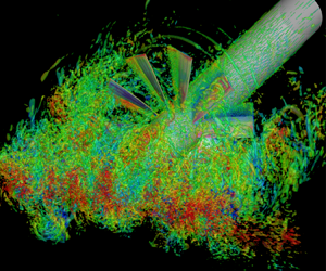
An instantaneous flow field for the zero-thrust case is illustrated in figure 6 from three different perspectives: a three-dimensional view and two plane views that are parallel and perpendicular to the wake, respectively. The isosurfaces of the Q-criterion show a wide range of flow structures interacting with the rotor. Tip vortices are also clearly visible in regions where they are not disrupted by the turbulent wake. The level of details of the flow structures captured by the simulation is well illustrated in this figure, and allows a detailed analysis of the broadband and tonal noise generation processes. The vortical structures around the thrusting rotor (not illustrated) show similar characteristics as in the zero-thrust case but are more elongated as they are drawn into the rotor.

Figure 6. Isosurfaces of  $Q$-criterion at
  $Q(R/U_{\infty })^2=1.2$ from different perspectives coloured by the velocity component perpendicular to the cylinder wake for the zero-thrust case (
 $J = 1.44$).
Figure 7 shows isocontours of the instantaneous radial vorticity on two cylindrical surfaces at  $r/R=1.26$ and
  $3.34$ for the zero-thrust case. The smaller surface is entirely immersed in the cylinder wake, and thus turbulence structures are observed around all blades. Due to the small radius, the blade chord Reynolds number based on the relative velocity
  $\sqrt {U^2_{\infty } + (\varOmega r)^2}$ is relatively low, and no trailing-edge vortex shedding is observed. In contrast, on the larger surface, which is close to the blade tip, not all blades are immersed in the wake at the same time, and the chord Reynolds number is significantly higher, leading to trailing-edge vortex shedding and associated noise as will be shown in the acoustic results.

Figure 7. Isocontours of instantaneous radial vorticity  $\omega _r R/U_{\infty }$ on two cylindrical surfaces for the zero-thrust case (
 $J = 1.44$). (a)
  $r/R=1.26$; (b)
  $r/R=3.34$.
Phase-averaged axial velocities at three different streamwise locations  $x/R=-0.38$, 0 and 0.38, which correspond to the blade leading edge at the root, rotor midplane and blade trailing edge at the root, respectively, are shown in figure 8 for both zero thrust and thrusting cases. The phase averaging is performed over 8.4 rotor rotations, or 84 blade passages for the zero-thrust rotor and
  $11.6$ rotor rotations, or
  $116$ blade passages for the thrusting rotor. The phase is selected such that two blades are aligned with the cylinder wake centreline in the rotor midplane. It can be seen that the thrusting rotor accelerates the flow mildly in the blade passage, whereas the zero-thrust rotor has a much smaller effect on the flow. Figure 9 depicts the phase-averaged turbulent kinetic energy at the same three streamwise locations. In contrast to the mean axial velocity, the turbulent kinetic energy is little affected by the rotor advance ratio except in the blade wake (figure 9c,f), where the thrusting rotor produces more turbulent kinetic energy due to its faster rotational speed.

Figure 8. Phase-averaged axial velocity  $U/U_{\infty }$ for the zero thrust (a–c) and thrusting (d–f) cases at different streamwise locations: (a,d)
  $x/R=-0.38$; (b,e)
  $x/R=0$; (c,f)
  $x/R=0.38$.

Figure 9. Phase-averaged turbulent kinetic energy  $\overline {u'_i u'_i}/(2U_{\infty }^2)$ for the zero thrust (a–c) and thrusting (d–f) cases at different streamwise locations: (a,d)
  $x/R=-0.38$; (b,e)
  $x/R=0$; (c,f)
  $x/R=0.38$.
5. Acoustic radiation
5.1. Results and validation
The radiated acoustic pressure for both the zero thrust and thrusting cases is computed using the blade surface pressure obtained from LES in (2.5) and (2.6) with  $N_s = 10$. Larger
  $N_s$ values of up to 200, which is the total number of grid cells along the blade span, as well as the alternative formulation (2.8) have been tested and shown no noticeable effects on results. The computed sound pressure levels (SPL) are compared with the single microphone measurements at VT (Alexander et al. Reference Alexander, Molinaro, Hickling, Murray, Devenport and Glegg2016, private communication 2016; Hickling et al. Reference Hickling, Alexander, Molinaro, Devenport and Glegg2017) at four positions on the port side (negative
  $y$ in figure 5) as listed in table 1 in dimensionless units. The observer angle,
  $\theta _o=\tan ^{-1}(y/x)$, is measured anticlockwise from the upstream direction, and the observer distance
  $r_o$ is defined as
  $r_o=\sqrt {x^2+y^2+z^2}$. The SPL are presented in decibels per Hz with reference to
  $2 \times 10^{-5}\ \textrm {Pa}$, and the frequency is normalized by the blade passing frequency,
  $f_{{BP}} = 10U_{\infty }/(D_r J)$. Note that the rotor diameter
  $D_r$ is related to the hub radius and the upstream-cylinder diameter by
  $D_r = 7.2R = 9D$. Since
  $U_{\infty } /R$ and
  $U_{\infty }/D$ are also used in this paper for frequency normalization, their relationships to
  $f_{{BP}}$ for both advance ratios are listed in table 2 for easy reference.
Table 1. Microphone locations for acoustic comparison with experimental data.

Table 2. Blade passing frequencies in terms of  $U_{\infty } /R$ and
  $U_{\infty }/D$.

The computed SPL for the zero-thrust case with and without contributions from the cylinder are presented in figure 10 along with the experimental data of Alexander et al. (Reference Alexander, Molinaro, Hickling, Murray, Devenport and Glegg2016, private communication 2016). The results cover nearly three decades of frequencies. Several important observations can be made from these results. The sound pressure spectra are broadband with a strong tonal peak at the cylinder vortex-shedding frequency (0.27 $f_{{BP}}$ based on LES data), a second peak at
  $f_{{BP}}$ caused by the rotor blades passing through the turbulent wake, and a third, minor peak at approximately
  $16f_{{BP}}$ due to vortex shedding from the blade trailing edge. The predicted trailing-edge shedding peak appears slightly more pronounced compared with the experimental spectra due to insufficient boundary-layer resolution as mentioned in § 4.1. By comparing the SPL with and without including contributions from the cylinder in the FW–H integral, it can be concluded that cylinder vortex shedding dominates the overall sound field at frequencies around and below the shedding frequency, whereas the rotor is the dominant sound source over higher frequencies starting at slightly below the BPF. Without accounting for the cylinder noise, the rotor-noise spectrum still exhibits a dominant, albeit lower peak, at the cylinder vortex-shedding frequency, which is caused by the interaction of the rotor with the large coherent vortices shed from the cylinder, and is analogous to the vortex-shedding peak of the airfoil noise in the rod–airfoil configuration (Jacob et al. Reference Jacob, Boudet, Casalino and Michard2005; Giret et al. Reference Giret, Sengissen, Moreau, Sanjosé and Jouhaud2015). Figure 10 demonstrates good overall agreement at all positions between numerical and single-microphone experimental data which include both rotor and cylinder noise. In particular, the blade-passing peak is captured very accurately. A slightly higher cylinder-shedding frequency is predicted by the LES, which is consistent with the velocity energy spectra shown in figure 4. The higher levels of experimental SPL at the low-frequency end is likely caused by extraneous noise sources. As shown by Alexander et al. (Reference Alexander, Molinaro, Hickling, Murray, Devenport and Glegg2016), the wind tunnel background noise rises rapidly below the cylinder shedding frequency and becomes dominant at 0.3–0.4 times the shedding frequency.

Figure 10. Sound pressure levels compared with experimental data and coarse-mesh LES results at four positions on the port side of the zero-thrust rotor: rotor noise (![]() , black); rotor+cylinder noise (
, black); rotor+cylinder noise (![]() , blue); rotor noise from coarse mesh LES (
, blue); rotor noise from coarse mesh LES (![]() , green); experiment (
, green); experiment (![]() , red) (Alexander et al. Reference Alexander, Molinaro, Hickling, Murray, Devenport and Glegg2016, private communication 2016). (a) Microphone 1; (b) Microphone 2; (c) Microphone 3; (d) Microphone 4.
, red) (Alexander et al. Reference Alexander, Molinaro, Hickling, Murray, Devenport and Glegg2016, private communication 2016). (a) Microphone 1; (b) Microphone 2; (c) Microphone 3; (d) Microphone 4.
The high-frequency limit for the turbulence-ingestion noise prediction can be estimated from the Nyquist wavelength of the nearly isotropic upstream grid and the convection velocity,  $f_c \sim U_c/(2\Delta x)$, where
  $U_c \approx \sqrt {U^2_{\infty } + (\varOmega R_{{tip}})^2}$ (see § 6). For
  $J=1.44$,
  $U_c \approx 2.41 U_{\infty }$, and hence the resolved frequency range of the acoustic spectra is
  $2.41$ times that of the energy spectra shown in figure 4. Given that the wake energy spectra are well resolved for
  $f\kern0.05em D/U_{\infty } \lesssim 3$, the sound pressure spectra are expected to be resolved for
  $f\kern0.05em D/U_{\infty } \lesssim 7.23$, or
  $f/f_{{BP}} \lesssim 9.37$. This is largely consistent with the results in figure 10 although, perhaps fortuitously, agreement with experimental data is also observed at frequencies beyond the trailing-edge vortex-shedding frequency due to contributions from self-noise.
To evaluate the grid sensitivity of the numerical results, a coarse-mesh LES is conducted for the zero-thrust rotor on a 16 million-cell mesh, which is generated by coarsening the original mesh by approximately a factor of two in each direction. The SPL of the rotor noise at the four microphone locations are also shown in figure 10. Since the coarser mesh captures only larger-scale turbulence structures, the resolved frequency range is reduced. Nonetheless, the agreement between the coarse and fine mesh results is excellent (within 1 dB) for nearly two decades of frequencies up to  $3f_{{BP}}$, and within 3 dB for frequencies up to
  $10f_{{BP}}$. The result of the grid-sensitivity study indicates that even this drastically coarsened mesh is capable of capturing the rotor turbulence-ingestion noise over the important low to mid-frequency range.
The numerical and experimental SPL for the thrusting case are compared in figure 11 at the same microphone locations as listed in table 1. Good agreement is again observed except at low frequencies due to wind tunnel noise in the experiment. Some discrepancies are also noted at high frequencies due to limited grid resolution. An estimate of the ingestion-noise frequency resolution based on  $U_c = 3.15 U_{\infty }$ for
  $J=1.05$ and the resolution limit of the wake energy spectra in figure 4,
  $f\kern0.05em D/U_{\infty } \lesssim 3$, indicates that the sound pressure spectra are well resolved for
  $f\kern0.05em D/U_{\infty } \lesssim 9.45$, or
  $f/f_{{BP}} \lesssim 8.93$. The high-frequency (
 $\,f/f_{BP} > 10$) tones in the experimental spectra are attributed to motor noise according to Alexander et al. (Reference Alexander, Molinaro, Hickling, Murray, Devenport and Glegg2016). Figure 12 compares the computed turbulence-ingestion noise levels for both advance ratios at microphone positions 1 and 4. Under thrusting condition at
  $J = 1.05$, the ingestion noise levels are approximately 5 dB higher than those under zero-thrust condition in the well-resolved mid-frequency range
  $1.32 \lesssim f\kern0.05em R/U_{\infty } \lesssim 9.0$. The BPF peak is more prominent, but as in the zero-thrust case no haystacking peaks at BPF harmonics are present because of the moderate thrust level. These observations are consistent with the experimental results of Alexander et al. (Reference Alexander, Molinaro, Hickling, Murray, Devenport and Glegg2016, private communication 2016).

Figure 11. Sound pressure levels compared with experimental data at four positions on the port side of the thrusting rotor: rotor noise (![]() , black); rotor+cylinder noise (
, black); rotor+cylinder noise (![]() , blue); experiment (
, blue); experiment (![]() , red) (Alexander et al. Reference Alexander, Molinaro, Hickling, Murray, Devenport and Glegg2016, private communication 2016). (a) Microphone 1; (b) Microphone 2; (c) Microphone 3; (d) Microphone 4.
, red) (Alexander et al. Reference Alexander, Molinaro, Hickling, Murray, Devenport and Glegg2016, private communication 2016). (a) Microphone 1; (b) Microphone 2; (c) Microphone 3; (d) Microphone 4.

Figure 12. Comparison of SPL of rotor noise under zero thrust and thrusting conditions at microphone positions 1 and 4:  $J = 1.44$ (
![]() , red);
, red);  $J = 1.05$ (
![]() , black). (a) Microphone 1; (b) Microphone 4.
, black). (a) Microphone 1; (b) Microphone 4.
Figure 13 shows the directivities of the dimensionless acoustic intensity,  $\overline {p^2}/(\gamma ^2 M_{\infty }^6 p^2_{\infty })$, for the zero thrust and thrusting cases at
  $r_o/R = 200$ in the
  $z=0$ and
  $y=0$ planes. There are two curves in each plot: the solid line is obtained by integrating the rotor-noise spectrum at each observer location over all frequencies up to 20
 $f_{{BP}}$ and represents the total noise, whereas the dashed line is based on integration from
  $0.5f_{{BP}}$ to 20
 $f_{{BP}}$ and thus excludes contributions from the tonal peak associated with Kármán vortices. The total noise and broadband noise intensities exhibit similar directivity patterns. As expected, the acoustic field is dominated by axial dipole radiation, but radiation in the two other directions is also significant. Note that the directivities in these two planes are expected to be symmetric with respect to the
  $x$-axis. The slight asymmetry exhibited in the figure is caused by imperfect statistical convergence.

Figure 13. Rotor noise directivity in terms of  $\overline {p^2}/(\gamma ^2 M_{\infty }^6 p_{\infty }^2)$ at
  $r_o/R = 200$ for the zero thrust and thrusting cases in: (a,b)
  $z=0$ plane; (c,d)
  $y=0$ plane. Over all frequencies
  $f\leqslant 20f_{{BP}}$ (
![]() , red); over frequencies
, red); over frequencies  $0.5 f_{{BP}}\leqslant f\leqslant 20 f_{{BP}}$ (
![]() , blue). (a,c)
, blue). (a,c)  $J = 1.44$; (b,d)
  $J = 1.05$.
5.2. Radiation from different blade regions
To examine the relative contributions to the radiated acoustic field from different blade regions, each blade is divided into five segments of equal width, numbered 1–5 from the root to the tip, along the radial direction. Figure 14 shows a comparison of the acoustic pressure spectra produced by these five segments for the zero thrust and thrusting cases at two observer locations  $z=0$,
  $r_o=200$,
  $\theta _o = 30^{\circ }$ and
  $75^{\circ }$. At both locations, the spectral level increases with the radial coordinate of the source region at frequencies higher than the BPF (
 $\,f_{{BP}} \approx 0.96 U_{\infty }/R$ for
  $J = 1.44$ and
  $1.32 U_{\infty }/R$ for
  $J = 1.05$). This increase is significantly larger at the shallower observer angle where the axial dipoles are more dominant, and slightly larger in the thrusting case compared with the zero-thrust case. A prominent spectral peak is seen at
  $f\kern0.05em R/U_{\infty }\approx 16.4$ and
  $21.8$ for
  $J = 1.44$ and
  $1.05$, respectively, for segments
  $4$ and
  $5$ but not others, indicating that the outer region is the dominant contributor to blade vortex shedding, which is consistent with the observation made in figure 7. In both cases at frequencies below the BPF, particularly at the cylinder shedding frequency, the spectral variation with segment position is less consistent and highly dependent on the observer angle. At
  $\theta _o=30^{\circ }$ the shedding peak varies only mildly and non-monotonically with the segment position, whereas at
  $\theta _o=75^{\circ }$ the shedding peak varies more significantly, showing mostly a decrease as the segment position varies from the root to the tip.

Figure 14. Contributions of different blade segments to rotor noise spectra for the zero thrust (a,b) and thrusting (c,d) cases in the  $z=0$ plane at
  $r_o/R=200$ and two observer angles. Segment 1 (
![]() , red); segment 2 (
, red); segment 2 (![]() , green); segment 3 (
, green); segment 3 (![]() , blue); segment 4 (
, blue); segment 4 (![]() , black); segment 5 (
, black); segment 5 (![]() , orange); entire rotor (
, orange); entire rotor (![]() , magenta). (a)
, magenta). (a)  $J = 1.44$,
  $\theta _o=30^{\circ }$; (b)
  $J = 1.44$,
  $\theta _o=75^{\circ }$; (c)
  $J = 1.05$,
  $\theta _o=30^{\circ }$; (d)
  $J = 1.05$,
  $\theta _o=75^{\circ }$.
6. Sears theory evaluation and analysis
6.1. Accuracy of Sears theory for rotor noise
As a classical model for airfoil-turbulence interaction noise, the Sears theory (Sears Reference Sears1941) provides a relationship between the unsteady lift of a thin airfoil and the upwash velocity encountered by the airfoil. It is of interest to evaluate its accuracy for predicting the noise of rotor ingesting the turbulent wake using the LES data. For a general two-dimensional gust the unsteady sectional lift  $L$ can be calculated from
 \begin{equation} L=\sum_{n=1}^N {\rm \pi}\rho_{\infty} C U_c \hat{v}_n \textrm{e}^{-\textrm{i}\omega_n t}S(\varOmega_n), \end{equation}
where  $C$ is the airfoil chord length,
  $U_c$ is the convection velocity,
  $\hat {v}_n$ is the upwash velocity component at angular frequency
  $\omega _n$, and
  $\varOmega _n=\omega _n C/(2U_c)$ is the reduced frequency. The Sears function is defined as
 \begin{equation} S(\varOmega_n)=\frac{2}{{\rm \pi} \varOmega_n [H_0^{(1)}(\varOmega_n)+i H_1^{(1)}(\varOmega_n)]}, \end{equation}
where  $H_0^{(1)}$ and
  $H_1^{(1)}$ are Hankel functions of the first kind. The summation in (6.1) is over all relevant Fourier modes, and the Fourier component of upwash velocity
  $\hat {v}_n$ is related to the time-domain upwash velocity
  $v_n(x,t)$ through
 \begin{equation} v_n(x,t)=\sum_{n=1}^{N} \hat{v}_n \exp\left({-\textrm{i}\omega_n(t-x/U_c)}\right). \end{equation}
 In the current implementation, the upwash velocity is defined as the component of the relative velocity perpendicular to the blade chord just upstream of the rotor and the convection velocity is defined as the velocity component parallel to the chord. During the flow simulation, the velocities in the rotor inlet plane, taken as  $x/R = -0.38$, are saved at every 16th time step. For each strip on the rotor blades, the convection velocity
  $U_c$ is estimated by
  $\sqrt {U_{\infty }^2+(\varOmega r)^2}$ in the middle of the strip, which is a good approximation of the spanwise-averaged, chord-parallel velocity at low angles of attack, and the upwash velocity
  $v_n$ at a given time is taken as the spanwise average of the upwash velocity. The unsteady lift for each strip is calculated using (6.1)–(6.3), summing up all the available Fourier modes, and the acoustic pressure is calculated using (2.5) and (2.6). Calculations have been performed using 10 strips and 118 strips along the blade span, and the resulting acoustic spectra are essentially the same.
Figure 15 shows, for both the zero thrust and thrusting cases, comparisons of the acoustic spectra predicted based on the unsteady loading from the Sears theory and that directly from the LES at  $r_o/R = 200$,
  $\theta _o = 45^{\circ }$. It is found that the Sears theory predicts the rotor noise reasonably well in the mid-frequency range of
  $0.7 \lesssim f\kern0.05em R/U_{\infty } \lesssim 12$ for
  $J = 1.44$ and
  $0.2 \lesssim f\kern0.05em R/U_{\infty } \lesssim 16$ for
  $J = 1.05$. The high-frequency bounds for the two cases are comparable in terms of
  $f/f_{BP}$ (
 ${\approx}12$), beyond which the Sears theory predictions fall off more quickly because they do not include the rotor self-noise. Large discrepancies are also seen between the Sears theory and LES predictions at low frequencies, particularly for the zero-thrust rotor. Similar comparisons are found at other observer angles.

Figure 15. Comparison of sound pressure spectra at  $r_o/R = 200$,
  $\theta _o = 45^{\circ }$ computed using blade unsteady loading from the Sears theory and LES for both advance ratios: Sears theory (
![]() , red); LES (
, red); LES (![]() , green). (a)
, green). (a)  $J=1.44$; (b)
  $J=1.05$.
6.2. Contribution from wake mean velocity defect
Since the Sears theory is linear, it allows an easy separation of the noise generated by the mean and fluctuating velocities in the wake. To this end the velocity in the rotor inlet plane is decomposed into a mean component and a fluctuating component, and their contributions to the sound pressure spectra are evaluated. The upwash velocity and its components caused by the mean and fluctuating wake velocities for the zero-thrust case are shown in figure 16 as a function of time at  $x/R = -0.38$,
  $r/R=2.3$ and 3. Since the outer region of the rotor blade enters and leaves the wake periodically, the mean component appears as a periodic signal in the rotor frame of reference. Comparing the velocities experienced by blades at the two radial locations, it can be seen that the mean velocity curve has longer bottoms at the outer position because the blade section spends more time outside the finite-thickness wake, and consequently, turbulent velocity fluctuations are seen during shorter time intervals. Velocity fluctuations are small when the blade is outside the wake at both locations.

Figure 16. Time history of the upwash velocity and its components caused by the mean and fluctuating wake velocities at  $x/R = -0.38$ and two radial positions: mean velocity (
![]() , red); fluctuating velocity (
, red); fluctuating velocity (![]() , blue); total velocity (
, blue); total velocity (![]() , green). The rotor advance ratio
, green). The rotor advance ratio  $J=1.44$. (a)
  $r/R = 2.3$; (b)
  $r/R = 3$.
The sound pressure spectra based on Sears theory predictions using the total upwash velocity and its mean and fluctuation components are compared in figure 17 for  $r_o/R = 200$,
  $\theta _o = 45^{\circ }$. The mean velocity defect in the wake is a major contributor to the BPF peak but produces negligible sound at other frequencies. This suggests the potential for using RANS simulations to predict the BPF tone (e.g. Moreau Reference Moreau2019a). The turbulent velocity fluctuations are responsible for the broadband sound at all frequencies.

Figure 17. Sound pressure spectra for  $J = 1.44$ predicted by the Sears theory at
  $r_o/R = 200$,
  $\theta _o = 45^{\circ }$ using the upwash velocity based on: total velocity (
![]() , red); mean velocity (
, red); mean velocity (![]() , green); fluctuating velocity (
, green); fluctuating velocity (![]() , blue).
, blue).
6.3. Mach number scaling
The Sears theory can be employed to derive the appropriate Mach number scaling of the acoustic pressure. Based on (6.1), the unsteady sectional lift  $L \sim \rho _{\infty } C U_{c} v_n$, and from (2.8), for
  $M_r \ll 1$,
 \begin{equation} p \sim \frac{1}{c_{\infty} r_d} \frac{\mathrm{d} F}{\mathrm{d} \tau} \sim \frac{1}{c_{\infty}} \frac{R}{r_d} \rho_{\infty} U^2_{{c}} v_n = \gamma p_{\infty} \frac{R}{r_d} \frac{U^2_{{c}}}{c^2_{\infty}} \frac{v_n}{c_{\infty}} \end{equation}
noting that  $F \sim LR$ (assuming the blade span
  $\sim R$),
  ${\mathrm {d}}/{\mathrm {d} \tau } \sim U_{{c}}/C$ and
  $c^2_{\infty } = \gamma p_{\infty }/\rho _{\infty }$. In (6.4) the convection velocity
  $U_{{c}} \approx \sqrt {U^2_{\infty } + (\varOmega r)^2}$, and the upwash velocity is dominated by turbulent fluctuations in the wake,
  $v_n \sim U_{\infty }$. Consequently,
  $p \sim (R/r_d) \gamma p_{\infty } M_{\infty } M^2_{{c}}$, where
  $M_{{c}} = U_{{c}}/c_{\infty }$. The acoustic pressure spectrum
  $\phi _{pp} \sim p^2/f$ with
  $f \sim U_{\infty }/R$ or
  $f_{{BP}}$, and therefore should scale with
  $M^2_{\infty } M^4_{{c}}$.
In figure 18 the rotor acoustic pressure spectra for  $J = 1.44$ and 1.05 are compared at microphone position 1 with different Mach number and frequency scalings. The Mach number
  $M_{{c}}$ is evaluated based on the convection velocity at the blade tip,
  $U_{{c}} = \sqrt {U^2_{\infty } + (\varOmega R_{{tip}})^2}$, since noise emission is dominated by the outer region of the rotor. It can be seen that unlike the
  $M^6_{\infty }$ scaling (figure 18a,c), the
  $M^2_{\infty } M^4_{{c}}$ scaling (figure 18b,d) successfully collapses the spectral curves for the two advance ratios in the frequency range between the BPF and the trailing-edge vortex shedding frequency, in which the Sears theory is accurate. The frequency scaling (
 $R/U_{\infty }$ vs.
  $f_{{BP}}$) also has an effect on the spectral level but it is less significant than the effect of Mach number scaling.

Figure 18. Sound pressure spectra for the zero thrust and thrusting cases at microphone position 1 with different Mach number and frequency scalings.  $J = 1.44$ (
![]() , red);
, red);  $J = 1.05$ (
![]() , black). (a)
, black). (a)  $M_{\infty }^6$ versus
  $U_{\infty }/R$ scaling; (b)
  $M_{\infty }^2 M_{{c}}^4$ versus
  $U_{\infty }/R$ scaling; (c)
  $M_{\infty }^6$ versus
  $f_{{BP}}$ scaling; (d)
  $M_{\infty }^2 M_{{c}}^4$ versus
  $f_{{BP}}$ scaling.
Figure 19 shows the  $M^2_{\infty } M^4_{{c}}$ scaled sound pressure spectra from three of the five blade segments shown in figure 14 for both rotor advance ratios. The local convection velocity,
  $U_{{c}} = \sqrt {U^2_{\infty } + (\varOmega r)^2}$ where
  $r$ is evaluated in the middle of the blade segment, is used to calculate
  $M_{{c}}$. At both observer locations illustrated in figure 19(a,b), there is a frequency range of approximately one decade (
 $0.8\text {--}8f_{{BP}}$ at
  $\theta _0 = 30^{\circ }$ and
  $1\text {--}10f_{{BP}}$ at
  $\theta _0 = 75^{\circ }$) within which all spectral curves for different blade regions (from the root to the tip) and different advance ratios show a reasonable collapse, in contrast to the spectral curves with
  $M^6_{\infty }$ scaling shown in figure 14. The collapse of the BPF peaks and broadband spectra in this frequency range also verifies that they are produced by turbulence ingestion and not by self-noise sources such as tip vortices and trailing-edge vortex shedding. The
  $M^2_{\infty } M^4_{{c}}$ scaling is invalid at high frequencies where the spectra are dominated by blade self-noise, and at low frequencies where the Sears theory prediction is inconsistent with simulation results.

Figure 19. Sound pressure spectra with  $M^2_{\infty } M^4_{{c}}$ scaling of the noise emitted from different blade segments for both
  $J = 1.44$ and 1.05, evaluated at
  $z = 0$,
  $r_o/R = 200$ and two observer angles. Segment 1,
  $J = 1.44$ (
![]() , black); segment 3,
, black); segment 3,  $J = 1.44$ (
![]() , black); segment 5,
, black); segment 5,  $J = 1.44$ (
![]() , black); segment 1,
, black); segment 1,  $J = 1.05$ (
![]() , red); segment 3,
, red); segment 3,  $J = 1.05$ (
![]() , red); segment 5,
, red); segment 5,  $J = 1.05$ (
![]() , red). (a)
, red). (a)  $\theta _o = 30^{\circ }$; (b)
  $\theta _o=75^{\circ }$.
It should be mentioned that although in figures 18 and 19 the  $M^2_{\infty } M^4_{{c}}$ scaling of rotor turbulence-ingestion noise is only verified for the
  $J = 1.44$ and 1.05 cases based on numerical simulation data, the VT experimental data (Alexander et al. Reference Alexander, Molinaro, Hickling, Murray, Devenport and Glegg2016, private communication 2016) contain a wider range of advance ratios from
  $J = 0.58$ to 1.44. An examination of the measured acoustic spectra indicates that this Mach number scaling is valid for rotor turbulence-ingestion noise at all the advance ratios tested in the experiment.
7. Unsteady sectional force analysis
As discussed in § 2.2, in the FW–H formulation of low-Mach-number turbulence ingestion noise, unsteady loading on the rotor blades is the dominant acoustic source, and the blade chord is often acoustically compact. In this case (2.4) can be rewritten as
 \begin{equation} p({\boldsymbol{x}}, t) = \frac{1}{4{\rm \pi} c_{\infty}} \frac{\partial}{\partial t} \sum_{n=1}^{N_b} \int_{R_{{hub}}}^{R_{{tip}}} \left[\frac{r_{d_i}}{r_d^2} \frac{f_i}{|1-M_r|} \right]_{\tau^{\ast}}^{n}\,\mathrm{d} r, \end{equation}
where  $f_i = \int p_{ij} n_j\,\mathrm {d}\varGamma$ is a line integral along the blade circumference representing the unsteady sectional force at radial position
  $r$. Based on (7.1), the radiated acoustic pressure spectrum can be represented in terms of the space–time correlations of the unsteady sectional force,
  $R_{ff}(r,\Delta r, \Delta t)$ (see, for example, Glegg et al. Reference Glegg, Devenport and Alexander2015). Likewise, using (2.7) the acoustic pressure spectrum can be related to the space–time correlations of the time derivative of the sectional force. In this section the spatiotemporal and spectral characteristics of the unsteady force and dipole source terms are examined.
To calculate the radial distributions of unsteady loading and dipole source, the sectional forces are evaluated at 100 equally spaced radial positions along the blade span in the following way: at each position, the surface pressure is interpolated from the LES surface grid onto the circumference of the blade cross-section. The sectional force is calculated by numerically integrating the surface pressure along the circumference. It is then projected onto the direction perpendicular to the chord. Only the chord-normal component, which is significantly larger than the chordwise component, is considered as in the formulation of Glegg et al. (Reference Glegg, Devenport and Alexander2015).
Figure 20 shows the blade spanwise distributions of the unsteady sectional force and dipole source spectra for both advance ratios at four discrete frequencies  $f_{{BP}}/2$,
  $f_{{BP}}$, 2
 $f_{{BP}}$ and 4
 $f_{{BP}}$. The chord-normal unsteady force is denoted as
  $L$, and its time derivative, denoted as
  $D_L = \mathrm {d} L/\mathrm {d} t$, is the corresponding dipole strength. In figure 20(a,c) the sectional force and dipole spectra, respectively, are plotted with the free stream Mach number
  $M^4_{\infty }$ scaling. The sectional-force spectral levels are slightly higher for the thrusting case than the zero-thrust case, whereas the sectional dipole spectral levels are significantly higher for the thrusting case due to the faster blade rotation and thus larger time derivative of
  $L$. Both the force and dipole levels increase with the radial coordinate until very close to the tip. Some weak oscillations are seen on the curves, particularly in the dipole spectra, due to limited statistical sampling period, but they do not obfuscate the variations with
  $J$ and
  $r$. Following the Sears theory analysis in § 6.3, it can be shown that more appropriate Mach number scalings for the force and dipole spectra are
  $M^2_{\infty } M^2_{{c}}$ and
  $M^4_{{c}}$, respectively, where
  $M_{{c}}$ is defined in terms of the local convection velocity,
  $U_{{c}} = \sqrt {U^2_{\infty } + (\varOmega r)^2}$. With these scalings, figure 20(b,d) shows generally good collapse of the
  $J = 1.44$ and 1.05 data, and both the force and dipole spectra exhibit smaller variations with the radial coordinate, except in the tip region.

Figure 20. Radial distributions of unsteady sectional force and dipole source spectra at four discrete frequencies. (a) Sectional force spectra with  $M^4_{\infty }$ scaling; (b) sectional force spectra with
  $M^2_{\infty } M_{{c}}^2$ scaling; (c) sectional dipole spectra with
  $M^4_{\infty }$ scaling; (d) sectional dipole spectra with
  $M_{{c}}^4$ scaling. Solid lines:
  $J = 1.44$; dashed lines:
  $J = 1.05$. In each plot from top to bottom:
  $f = f_{{BP}}/2$,
  $f_{{BP}}$,
  $2 f_{{BP}}$,
  $4 f_{{BP}}$.
The space–time correlation coefficient of the chord-normal unsteady blade sectional force involving different blades is defined as
 \begin{equation} C_{LL}^{(m,n)}(r,\Delta r,\Delta t)=\frac{\overline{L^{(m)}(r,t)L^{(n)}(r+\Delta r,t+\Delta t)}}{\sqrt{\overline{(L^{(m)}(r,t))^2}}\sqrt{\overline{(L^{(n)}(r+\Delta r,t+\Delta t))^2}}}, \end{equation}
where  $m$ and
  $n$ are blade numbers, and the overbar denotes averaging over time and 10 blades in the present calculation. Figure 21 shows for both advance ratios correlations between the sectional force in the middle of a blade (
 $r/R = 2.3$) and those on either the same blade or neighbouring blades in the forward direction at varying radial and temporal separations. From these results, it can be seen that the correlations between different blades decrease as their separation increases. The maximum correlation with the immediate neighbour is 0.61 for
  $J = 1.44$ and 0.66 for
  $J = 1.05$, and with the second neighbour it is reduced to 0.48 and 0.47, respectively. The space–time correlations for the sectional dipole sources
  $D_L$, defined in the same way as in (7.2), are shown in figure 22 for the same blade and immediate neighbouring blades. The blade-to-blade dipole correlations are much weaker than the force correlations, with maximums of 0.16 for
  $J = 1.44$ and 0.18 for
  $J = 1.05$ between immediate neighbours and even smaller values between second neighbours (not shown). This is because the time derivative places more weights on smaller scales. By comparing the correlation contours for the two advance ratios, it is observed that blade-to-blade correlations are mildly stronger in the thrusting case because the blades pass through the wake faster, and the correlation times are comparable in terms of the blade passing time. Note that the correlation levels increase periodically at time separations equal to approximately half the rotation period for both advance ratios, which is caused by the blades cutting through the opposite sides of the wake. On the same blade the radial correlation lengths are comparable for the two advance ratios.

Figure 21. Space–time correlation coefficient,  $C_{LL}^{(m,n)}(r/R = 2.3, \Delta r, \Delta t)$, of the unsteady sectional force on blades for (a,c,e)
  $J = 1.44$ and (b,d,f)
  $J = 1.05$. (a,b)
  $C_{LL}^{(1,1)}$; (c,d)
  $C_{LL}^{(1,2)}$; (e,f)
  $C_{LL}^{(1,3)}$.

Figure 22. Space–time correlation coefficient,  $C_{D_L D_L}^{(m,n)}(r/R = 2.3, \Delta r, \Delta t)$, of the unsteady sectional dipole on blades for (a,c)
  $J = 1.44$ and (b,d)
  $J = 1.05$. (a,b)
  $C_{D_L D_L}^{(1,1)}$; (c,d)
  $C_{D_L D_L}^{(1,2)}$.
Figure 23 shows the coherence of blade sectional forces for both the zero thrust and thrusting cases. The coherence between the sectional force at  $r/R = 2.3$ on a blade and those at other radial locations on the same blade is shown in figure 23(a,b). With the frequency normalized by the BPF, the coherence patterns are very similar for both advance ratios, which indicates that the dipole source coherence on the same blade is primarily determined by the rotational speed (see also Wang Reference Wang2017). The coherence length decays quickly with frequency and becomes very small beyond 2
 $f_{{BP}}$. Figure 23(c,d) shows the corresponding coherence with the neighbouring blade in the forward direction. The blade-to-blade coherence shows stronger dependence on the rotor advance ratio but its value is small. The maximum coherence occurs at frequencies below the BPF and is no larger than 0.3. At higher frequencies the coherence is practically zero. Same blade and blade-to-blade coherence involving origins in outer blade regions (e.g.
  $r/R = 3$) has also been examined, and very similar results are obtained. The coherence length exhibits a modest increase with the radial coordinate
  $r$ until the upper side is affected by the unsteady flow around the tip. Note that for stationary turbulence, it can be shown theoretically (e.g. Yang & Wang Reference Yang and Wang2013) that the dipole coherence is identical to the force coherence, and hence the results in figure 23 also apply to blade sectional dipoles. The small blade-to-blade sectional dipole correlations and coherence demonstrate that different blades act as nearly independent acoustic sources, at least for frequencies higher than the BPF. This also explains the absence of haystacking peaks at harmonics of the BPF at the two advance ratios considered.

Figure 23. Coherence between the unsteady sectional force at  $r/R = 2.3$ and those at different radial positions on (a,b) the same blade,
  $\gamma^{2(1,1)}_{LL}$, and (c,d) forward neighbouring blade,
  $\gamma^{2(1,2)}_{LL}$, for (a,c)
  $J = 1.44$ and (b,d)
  $J = 1.05$.
8. Distortions of wake turbulence
In theoretical models based on gust-response theory for turbulence-ingestion noise such as those by Sears (Reference Sears1941), Amiet (Reference Amiet1975) and Glegg et al. (Reference Glegg, Devenport and Alexander2015), a key input is the upwash velocity upstream of the rotor. As discussed in the introduction, an important issue is how significantly the incoming turbulence is distorted as it is ingested into the rotor and whether or not the distortion must be taken into account in the noise prediction. To address this issue, in this section the distortion of wake turbulence by the rotor is evaluated by examining the two-point and space–time correlations of the upwash velocity field in comparison with those of the undistorted field, and the noise predictions using distorted and undistorted upwash velocities are compared.
To establish the undistorted reference flow, a simulation without the rotor is carried out with other conditions, including the computational domain size, grid resolution and turbulent inflow, kept the same as in the zero-thrust rotor simulation. The total number of control volumes is 53 million. Figure 24 shows the r.m.s. values of the upwash velocity at  $x/R = -0.38$, which corresponds to the blade leading edge at the root, from the simulations with and without the rotor. Each plot covers the entire rotor disk from the hub (the white circle in the middle) to the blade tip (the outer circle). It can be seen that in the presence of the rotor, the upwash velocity is amplified near the hub by the hub-wall boundary-layer turbulence. The faster rotational speed in the
  $J = 1.05$ case induces stronger velocity fluctuations in a thicker region around the hub compared with the
  $J = 1.44$ case. The upwash velocity is also increased in the entire rotor plane due to the blade rotation, and the increase is larger for the thrusting rotor.

Figure 24. Isocontours of the r.m.s. of upwash velocity at  $x/R = - 0.38$ computed with and without the rotor. (a) With rotor,
  $J = 1.44$; (b) with rotor,
  $J = 1.05$; (c) without rotor.
Two-point correlations of the upwash velocity are calculated using
 \begin{equation} C_{v_n v_n}(x,r,\theta,\Delta r,\Delta\theta) = \frac{\overline{v_n(x,r,\theta,t) v_n(x,r+\Delta r,\theta+\Delta\theta,t)}}{\sqrt{\overline{v^2_n(x,r,\theta,t)}}\sqrt{\overline{v^2_n(x,r+\Delta r,\theta+\Delta\theta,t)}}}, \end{equation}
where the overbar denotes averaging over time and symmetric locations in the azimuthal direction, and  $x$,
$x$,  $r$ and
  $\theta$ are the streamwise, radial and azimuthal coordinates, respectively. Figure 25 shows the two-point correlations of the upwash velocity in two planes,
  $x/R = -1.32$ and
  $-0.38$, at
  $r/R = 3$,
  $\theta = 90^{\circ }~(y = 0)$. The first plane is one chord length upstream of the blade leading edge and the second plane is at the leading edge at the root. In both planes the correlation lengths appear slightly larger in both the radial and azimuthal directions with the rotor present but the difference is relatively small. Two negative correlation stripes are observed in the plane close to the rotor with the rotor present due to fluid motions induced by the blade rotation.

Figure 25. Two-point correlations of the upwash velocity,  $C_{v_n v_n}(\Delta y, \Delta z)$, at (a–c)
  $x/R = -1.32$; (d–f)
  $x/R = -0.38$,
  $r/R = 3$,
  $\theta = 90^{\circ }$ with and without the rotor. (a,d) With rotor,
  $J = 1.44$; (b,e) with rotor,
  $J = 1.05$; (c,f) without rotor.
Turbulence distortions by the rotor are further examined in terms of the radial spatial-temporal correlations of the upwash velocity, defined as
 \begin{equation} C_{v_n v_n}(x,r,\theta,\Delta r,\Delta t) = \frac{\overline{v_n(x,r,\theta,t) v_n(x,r+\Delta r,\theta,t+\Delta t)}}{\sqrt{\overline{v^2_n(x,r,\theta,t)}}\sqrt{\overline{v^2_n(x,r+\Delta r,\theta,t+\Delta t)}}}, \end{equation}
at the same two locations,  $x/R = -1.32$ and
  $-0.38$,
  $r/R = 3$,
  $\theta = 90^{\circ }$. As shown in figure 26, at the upstream station
  $x/R = -1.32$, the shapes of the correlation contours with and without the rotor are similar with only small changes in the radial correlation length, indicating no significant distortions at this location. With the rotor present, at the root leading-edge position
  $x/R = -0.38$, there are multiple stripes in correlation contours caused by blades passing through the wake. The temporal spacing between the stripes is the blade passage time and therefore smaller for the smaller
  $J$ case. The main features of the correlation contours in the middle show that the time scale is reduced by the rotor, particularly for the
  $J = 1.05$ case, while the radial correlation length scale is increased slightly by the rotor, which is consistent with figure 25(d–f). Note that the reduction in correlation time is caused by blade rotation due to proximity to the rotor and not by the type of distortion due to mean streamtube contraction as discussed by Hanson (Reference Hanson1974) and Majumdar & Peake (Reference Majumdar and Peake1998). The small turbulence distortions found in this study are consistent with the analysis of Majumdar & Peake (Reference Majumdar and Peake1998), given the (nominally) zero and moderate thrust levels of the rotor at the two advance ratios.

Figure 26. Space–time correlations of the upwash velocity,  $C_{v_n v_n}(\Delta r, \Delta t)$, at (a,c,e)
  $x/R = -1.32$; (b,d,f)
  $x/R = -0.38$,
  $r/R = 3$,
  $\theta = 90^{\circ }$ with and without the rotor. (a,b) With rotor,
  $J = 1.44$; (c,d) with rotor,
  $J = 1.05$; (e,f) without rotor.
To investigate the effect of turbulence distortions on noise prediction, the far-field acoustic pressure is calculated based on the unsteady loading predicted by the Sears theory using the upwash velocities from the LES with and without the rotor. The results are compared with that based on the unsteady loading directly from the LES in figure 27(a,b) for the zero thrust and thrusting cases, respectively, at the observer location  $r_o/R = 200$,
  $\theta _o = 45^{\circ }$. In the mid-frequency range where the Sears theory provides reasonable predictions, the Sears results based on the upwash velocity with the rotor present agree slightly better with the LES prediction, indicating that accounting for turbulence distortions by the rotor provides a small improvement to the noise prediction.

Figure 27. Sears theory predictions of sound pressure spectra at  $r_o/R = 200$,
  $\theta _o = 45^{\circ }$ using upwash velocities from LES with and without the rotor: without rotor (
![]() , red); with rotor (
, red); with rotor (![]() , blue); LES result (
, blue); LES result (![]() , black). (a)
, black). (a)  $J = 1.44$; (b)
  $J = 1.05$.
9. Conclusion
In this study the turbulence-ingestion noise produced by a 10-bladed rotor in the wake of a circular cylinder is investigated numerically at two rotor advance ratios. The cylinder, whose diameter is  $1/9$ of the rotor diameter, is located
  $20$ cylinder diameters upstream of the rotor centre. The Reynolds number based on the free stream velocity and the rotor diameter is
  $5.83 \times 10^5$, and the free stream Mach number is
  $0.058$.
Large-eddy simulations are performed to obtain a detailed spatiotemporal description of the rotor–wake interaction. The acoustic field is computed using the FW–H equation with blade unsteady loading as the dominant noise source. The results demonstrate that this methodology is capable of computing the rotor turbulence-ingestion noise accurately. The predicted SPL agree well with the VT experimental measurements over a wide range of frequencies at various observer locations. The acoustic spectra are broadband with a strong tonal peak at the cylinder vortex-shedding frequency, a second peak at the BPF, and a minor peak at the blade vortex-shedding frequency. Consistent with the experimental measurements, a thrusting rotor at advance ratio  $J = 1.05$ is found to produce a 4–6 dB increase in ingestion noise compared with a zero-thrust rotor at
  $J = 1.44$ in the frequency range of 1–10 times the BPF.
The LES flow-field and surface-pressure data are used to analyse the acoustic source characteristics and mechanisms. It is shown that the blade dipole source strength, and hence the radiated acoustic power, increase with distance to the hub until near the blade tip. Blade-to-blade correlations and coherence of dipole sources are small. The accuracy of the Sears theory for rotor turbulence-ingestion noise prediction is evaluated using the upwash velocity obtained from the LES. The Sears theory provides a reasonable prediction in the mid-frequency range but is unsatisfactory at low and high frequencies. Guided by the theory, the Mach number scaling of the turbulence-ingestion noise spectra is identified as  $M^2_{\infty } M^4_{{c}}$, where
  $M_{{c}}$ is based on the free stream velocity relative to the blade. The contributions from the mean and fluctuating velocities in the wake to the rotor noise are evaluated separately, and it is found that the mean wake velocity defect only contributes to the ingestion noise at the BPF. Turbulence distortions by the rotor are found to be small at the two advance ratios considered, and their inclusion in the upwash velocity only provides a small improvement to the accuracy of noise prediction using the Sears theory.
Acknowledgements
This research was supported by the Office of Naval Research under Grants N00014-14-1-0129 and N00014-17-1-2493, with K.-H. Kim as Program Officer. Computer time was provided by the US Department of Defense High Performance Computing Modernization Program and Center for Research Computing at the University of Notre Dame. The authors gratefully acknowledge W. Devenport and N. Alexander for providing experimental data and helpful discussions, and W. Blake and S. Glegg for valuable discussions. Portions of this work were presented in AIAA Paper 2016-2998, 22nd AIAA/CEAS Aeroacoustics Conference, Lyon, France, 30 May–1 June 2016 and AIAA Paper 2017-3533, 23rd AIAA/CEAS Aeroacoustics Conference, Denver, Colorado, 5–9 June 2017.
Declaration of interests
The authors report no conflict of interest.


