


1. Introduction
Shock wave/boundary layer interactions (SWBLIs) are ubiquitous in internal and external flow fields of aerospace and aeronautic applications, such as transonic aerofoils, supersonic inlets and over-expansion nozzles (Green Reference Green1970). In the interaction regions, an adverse pressure gradient provoked by shock waves often thickens the boundary layer, causing the latter to be unsteady and even separated. However, the shock-induced separations are generally detrimental to an aircraft. For example, SWBLIs on an aerofoil will increase the drag; concurrently, the accompanying unsteady aerodynamic force and thermal load will affect directly the performance and fatigue life of the aerofoil structures (Dolling Reference Dolling2001; Anderson Reference Anderson2010). In addition, SWBLIs affect adversely the internal flow field in a supersonic inlet, resulting in a considerable loss in total pressure, an increase in the flow distortion, a complicated accompanying shock wave system and formation of the aerodynamic throat. Owing to these factors, the supersonic inlet is under an off-design state, leading to a significant performance degradation of the propulsion system (Babinsky & Ogawa Reference Babinsky and Ogawa2008; Krishnan, Sandham & Steelant Reference Krishnan, Sandham and Steelant2009).
Since the pioneering work by Ferri (Reference Ferri1940), SWBLIs have been investigated extensively to elucidate the complex physical mechanism, wherein the most frequently encountered interactions are shock wave/turbulent boundary layer interactions (SWTBLIs), although shock wave/laminar or transition boundary layer interactions have also been investigated in the literature. According to the type of shock wave and the application geometry, SWBLIs can be categorised into various forms, such as incident SWBLI (ISWBLI), compression ramp-induced SWBLI (CRSWBLI), normal SWBLI and swept SWBLI. In particular, ISWBLIs and CRSWBLIs have attracted considerable attention owing to their simple configuration and quasi-two-dimensional properties (Dolling Reference Dolling2001; Babinsky & Harvey Reference Babinsky and Harvey2011). In the past decades, numerous theoretical, experimental and numerical studies have been conducted on these two categories of interactions, yielding several canonical conclusions on various flow features, including the mean flow configuration (Henderson Reference Henderson1967; Settles Reference Settles1976; Viswanath Reference Viswanath1988; Zheltovodov Reference Zheltovodov2006; Délery & Dussauge Reference Délery and Dussauge2009), pressure distribution (Chapman, Kuehn & Larson Reference Chapman, Kuehn and Larson1957; Erdos & Pallone Reference Erdos and Pallone1962; Carrière, Sirieix & Solignac Reference Carrière, Sirieix and Solignac1969; Charwat Reference Charwat1970; Matheis & Hickel Reference Matheis and Hickel2015) and low-frequency unsteadiness (Dupont, Haddad & Debiève Reference Dupont, Haddad and Debiève2006; Pirozzoli & Grasso Reference Pirozzoli and Grasso2006; Ganapathisubramani, Clemens & Dolling Reference Ganapathisubramani, Clemens and Dolling2007; Dussauge & Piponniau Reference Dussauge and Piponniau2008; Wu & Martín Reference Wu and Martín2008; Piponniau et al. Reference Piponniau, Dussauge, Debiève and Dupont2009; Souverein et al. Reference Souverein, van Oudheusden, Scarano and Dupont2009; Touber & Sandham Reference Touber and Sandham2009; Souverein et al. Reference Souverein, Dupont, Debieve, Dussauge, van Oudheusden and Scarano2010; Touber & Sandham Reference Touber and Sandham2011; Priebe & Martín Reference Priebe and Martín2012; Clemens & Narayanaswamy Reference Clemens and Narayanaswamy2014; Priebe et al. Reference Priebe, Tu, Rowley and Martín2016; Adler & Gaitonde Reference Adler and Gaitonde2018).
The scale of the separated flow induced by SWBLIs is crucial for the geometric design of aeronautical applications. Previous experimental studies have shown that the free-stream Mach number, Reynolds number and deflection angle significantly influence the scale of the separated flow (Thomke & Roshko Reference Thomke and Roshko1969; Spaid & Frishett Reference Spaid and Frishett1972; Settles, Bogdonoff & Vas Reference Settles, Bogdonoff and Vas1976). According to the numerical simulation data, Ramesh & Tannehill (Reference Ramesh and Tannehill2004) established a correlation function that depends on free-stream Mach number, Reynolds number and specific pressure rise to evaluate the streamwise extent of the separation in SWTBLIs. A new scaling approach for the interaction length was derived by Souverein, Bakker & Dupont (Reference Souverein, Bakker and Dupont2013) based on the mass conservation law. By using the non-dimensional shock strength metric and non-dimensional interaction length, the new method can reconcile effectively the variations in experimental and numerical data of ISW/turbulent boundary layer interactions (ISWTBLIs) and compression ramp-induced shock wave/turbulent boundary layer interactions (CRSWTBLIs) with different Mach numbers, Reynolds numbers and geometric configurations. Moreover, heat transfer also plays a significant role in the extent of shock-induced separation (Babinsky & Harvey Reference Babinsky and Harvey2011). The recent studies indicated that the applicability of the adiabatic scaling method by Souverein et al. (Reference Souverein, Bakker and Dupont2013) is limited in hypersonic SWTBLIs in which the heat transfer generally cannot be ignored (Helm Reference Helm2021; Helm & Martín Reference Helm and Martín2021; Hong, Li & Yang Reference Hong, Li and Yang2021). Hong et al. (Reference Hong, Li and Yang2021) found that the relationship between the non-dimensional parameters proposed by Souverein was not accurate enough for hypersonic SWTBLIs. They corrected the new non-dimensional shock strength metric and identified two scaling relationships of the non-dimensional parameters in hypersonic SWTBLIs according to different Reynolds numbers. The study by Helm & Martín (Reference Helm and Martín2021) performed a control volume analysis and derived the corresponding separation length scaling for an axisymmetric cylinder-with-flare geometry (a geometry used commonly in hypersonic cases, see Brooks et al. Reference Brooks, Gupta, Marineau, Martín, Smith and Marineau2017). Considering the difference between the skin friction coefficients in adiabatic and non-adiabatic wall conditions, they modified the scaling method of Souverein et al. (Reference Souverein, Bakker and Dupont2013) and put forward a new generalised scaling method to analyse the data compilation of both the supersonic and hypersonic SWTBLIs with various wall heat transfer conditions. The new generalised scaling of the SWTBLI database (including two-dimensional compression ramp and axisymmetric cylinder-flare cases) showed a linear collapse for all incipiently separated SWTBLI data but a significant spreading in the fully separated regime. Based on the large eddy simulation database, they analysed the physical mechanisms for the two SWTBLI regimes. The result indicated that the momentum distribution in the incoming boundary layer is a crucial factor influencing separation length scaling in the incipiently separated regime; in contrast, the presence and strength of inviscid vortical structures affect significantly the separation length for fully separated cases.
Note that in the aforementioned studies, the separated flows are induced commonly by a single shock wave. However, in the internal compression process of a supersonic mixed-compression inlet with a high Mach number, the multi-stage compression induced by shock waves is often used to efficiently decelerate and pressurise the supersonic airflow (Sanders & Weir Reference Sanders and Weir2008; Tan, Sun & Huang Reference Tan, Sun and Huang2012; Huang et al. Reference Huang, Tan, Sun and Sheng2017). These shock waves inevitably interact with the boundary layer in the channel and induce multi-SWBLIs. For instance, the cowl shock wave and downstream contour-induced shock wave impinge sequentially on the boundary layer on the ramp-side surface. When the two shock interaction regions are close, they combine to form a large-scale separation (Tan et al. Reference Tan, Sun and Huang2012; Huang et al. Reference Huang, Tan, Sun and Sheng2017). Recently, Li et al. (Reference Li, Tan, Zhang, Huang, Guo and Lin2020) employed the ice-cluster-based planar laser scattering (IC-PLS) technique to visualise the flow field of dual-ISWTBLIs in a Mach 2.48 flow with the two deflection angles  $8^\circ$ and
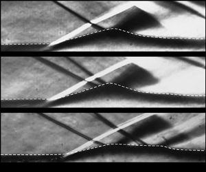
  $5^\circ$. Such a study indicated that the distance between the two incident shock waves (ISWs) affected significantly the overall separation region. According to the shape of the separation bubble, the dual-ISWTBLI flow was of three kinds. The first was a strong coupling separated flow with a triangle-like separation bubble while the shock distance was 0 (figure 1a). As the shock distance increased to four times the boundary layer thickness, the shape of the separation bubble changed to quadrilateral-like, yielding the second kind of dual-ISWTBLI (figure 1b). When the shock distance was sufficiently large (eight times the boundary layer thickness), the third kind of dual-ISWTBLI was formed with the decoupling of the two isolated single-ISWTBLIs (figure 1c). Under the specific experimental condition in the third kind of dual-ISWTBLI in that study, the adverse pressure gradient in the two single-ISWTBLIs was insufficient to induce a fully separated flow, so there are no visible separation bubbles in figure 1(c). Moreover, Zhang et al. (Reference Zhang, Li, Tan, Sun, Wu and Zhang2021) presented the three-dimensional structures in dual-swept SWTBLIs, thereby showing that the separated flow in the wall vicinity was extremely complicated. The overall flow can be regarded as a combination of three interactions induced by the first, second and converged swept shock waves; these interactions provoked the corresponding separation and rear shock waves, which interacted with each other and afforded a spatially intricate shock wave system.

Figure 1. IC-PLS images of three kinds of dual-ISWTBLI (Li et al. Reference Li, Tan, Zhang, Huang, Guo and Lin2020). (a) First kind of dual-ISWTBLI, with  $Ma_0 = 2.48$,
  $\alpha _1 = 8^\circ$,
  $\alpha _2 = 5^\circ$ and
  $d = 0\delta _0$. (b) Second kind of dual-ISWTBLI, with
  $Ma_0 = 2.48$,
  $\alpha _1 = 8^\circ$,
  $\alpha _2 = 5^\circ$ and
  $d = 4\delta _0$. (c) Third kind of dual-ISWTBLI, with
  $Ma_0 = 2.48$,
  $\alpha _1 = 8^\circ$,
  $\alpha _2 = 5^\circ$ and
  $d = 8\delta _0$. The symbols
  $Ma_0$,
  $\alpha _1$,
  $\alpha _2$,
  $d$ and
  $\delta _0$ denote the free-stream Mach number, first deflection angle, second deflection angle, shock distance and boundary layer thickness, respectively.
The multi-SWTBLI flow is ubiquitous in the supersonic mixed-compression inlet, and the sub-interaction regions often combine to form a fairly complex separated flow (Gaitonde Reference Gaitonde2015). The interaction of the turbulent boundary layer with dual-ISWs is one of the simplest forms of the multi-SWTBLIs. However, the previous study on dual-ISWTBLIs (Li et al. Reference Li, Tan, Zhang, Huang, Guo and Lin2020) was based solely on IC-PLS images, and quantitative analysis of the effect of shock distance on the flow features (such as the exact extent of the reverse flow region and wall pressure distribution) was not available. Therefore, to study quantitatively the flow mechanism involved in the dual-ISWTBLIs, this paper performs a comparative investigation on single-ISWTBLIs and dual-ISWTBLIs with identical total deflection angles by using schlieren photography, wall-pressure measurement and surface oil-flow visualisation. Since the third kind of dual-ISWTBLI can be regarded as two isolated single-ISWTBLIs, its flow features can be described by referring to the single-ISWTBLI theory reported in the literature. Therefore, this study focuses on only the first and second kinds of dual-ISWTBLIs, in which the coupling of the two sub-interactions leads to complex separation configurations. First, the impingement points of the two ISWs were ensured to intersect on the bottom wall to yield the first kind of dual-ISWTBLI. The similarities and differences between the first kind of dual-ISWTBLI and the single-ISWTBLI with an identical total deflection angle condition were analysed. Then the distance between the two ISWs was increased to explore its effect on the separation flow. Based on the free-interaction theory, an inviscid simplified model was developed for dual-ISWTBLI flow to describe the separation configurations, based on which the factors influencing the shape of the separation bubble were investigated in detail.
2. Experimental methodology
2.1. Wind tunnel and test model
Experiments were performed in a wind tunnel at Nanjing University of Aeronautics and Astronautics. The wind tunnel is a free-jet type with an atmospheric environment upstream and a  $300~{\rm m}^{3}$ vacuum spherical tank downstream. When the wind tunnel is in operation, a uniform supersonic flow of Mach 2.73 is produced downstream of the Laval nozzle. The exit section of the nozzle is a square with dimensions
  $200 \times 200\ {\rm mm}^{2}$. The operating time of the wind tunnel is 14 s. The total pressure of supersonic flow is
  $100 \pm 0.3\ {\rm kPa}$, the total temperature is
  $286 \pm 1.5\ {\rm K}$ and the unit Reynolds number is approximately
  $9.2 \times 10^6\ {\rm m}^{-1}$.
Figure 2(a) is a picture of the test model in the wind tunnel, which mainly comprised a shock generator, two sidewalls embedded with optical glass and a bottom wall. Figures 2(b) and 2(c) are schematics of the test model and its relative position with the Laval nozzle, respectively. In this study, the spanwise width between the two sidewalls is 140 mm. The leading edges of the sidewall and bottom wall are unaligned, with the former 90 mm downstream of the latter. The short-sidewall arrangement is adopted to restrict the development of the sidewall boundary layer, thereby decreasing the sidewall effect on the flows in the central region. The pre-test indicated that the boundary layer 150 mm downstream of the leading edge of the bottom wall maintained a laminar state. Therefore, a rough band is set 10 mm downstream of the leading edge of the bottom wall to promote the boundary layer transition and ensure that the boundary layer upstream of the SWBLI is turbulent. The spanwise width of the front part of the bottom wall is 160 mm, and two winglets are installed on both sides to prevent the potential lateral flow from disturbing the incoming boundary layer.

Figure 2. Experimental set-up of the working section: (a) picture of the test model; (b) schematic diagram of the test model; (c) relative position of the test model and Laval nozzle.
2.2. Shock generator
In this study, single-ISWTBLIs and dual-ISWTBLIs were investigated. The single-ISW and dual-ISWs were generated using a single-ramp wedge and a dual-ramp wedge, respectively. A schematic of the shock generator is depicted in figure 3. In fact, the single-ISWTBLI can be regarded as a particular case of the dual-ISWTBLIs when the first or second deflection angle is  $0^\circ$. Geometric parameters of nine shock generators are listed in table 1, including the leading edge height (
 $h$), spanwise width (
 $w$), total deflection angle (
 $\alpha _t$), first deflection angle (
 $\alpha _1$), second deflection angle (
 $\alpha _2$), length of the first ramp (
 $l_1$), and length of the second ramp (
 $l_2$). As shown in figure 3, in the dual-ISWTBLIs, two inviscid ISWs intersect the centreline of the bottom wall at the points
  $O_1$ and
  $O_2$, respectively. The distance between
  $O_1$ and
  $O_2$ is defined as the shock distance
  $d$ (where
  $d=x_{O2}-x_{O1}$). Among the tests, cases 1–3 correspond to single-ISWTBLIs with deflection angles
  $10^\circ$,
  $11^\circ$ and
  $12^\circ$, respectively. Cases 4–7 correspond to dual-ISWTBLIs with total deflection angles
  $12^\circ$,
  $12^\circ$,
  $11^\circ$ and
  $10^\circ$, respectively; and the shock distance in the four cases was set to 0 mm to form the first kind of dual-ISWTBLIs. Then, in cases 8 and 9, the shock distance
  $d$ was enlarged to a moderate value to form the second kind of dual-ISWTBLIs with different deflection angle combinations: (
 $\alpha _1 = 5^\circ$,
  $\alpha _2 = 7^\circ$) and (
 $\alpha _1 = 7^\circ$,
  $\alpha _2 = 5^\circ$), respectively. In dual-ISWTBLIs, the adjustment of
  $d$ was achieved by changing the length of the first ramp. Due to the elongation of the shock generator along the streamwise direction in cases 8 and 9, the leading edge height of the shock generator
  $h$ was increased appropriately to avoid the unstart state owing to the large contraction ratio of the channel. Constrained by the test model's geometry, the coordinate of point
  $O_1$ in the case of single-ISWTBLIs was 255 mm downstream of the leading edge of the bottom wall, whereas the coordinate of point
  $O_1$ in the case of dual-ISWTBLIs was 265 mm downstream of the leading edge of the bottom wall. Therefore, the origin of the coordinate system in each case was set at point
  $O_1$ to facilitate comparisons between different cases. Also, as shown in figure 2(b), the
  $x$-,
$x$-,  $y$- and
  $z$-axes correspond to the streamwise, wall-normal and spanwise directions, respectively.

Figure 3. Schematic of shock generator.
Table 1. Geometric parameters of shock generators.

2.3. Experimental measurement methods
We detected the flow fields using a combination of schlieren photography, static pressure measurement and surface oil-flow visualisation.
Schlieren photography is an optical measurement method commonly used to study SWBLI flows. Schlieren images can reflect the density gradient of the airflow such that the shock waves, expansion waves and shear layer can be visualised. As shown in figure 4, the schlieren system in this experiment has a classical ‘Z-type’ configuration, with a xenon lamp point light source, a pair of concave mirrors with 200 mm diameter and 2000 mm focal length, a knife edge and a high-speed camera. The first concave mirror reflected the emanative light from the point light source into parallel light rays, which then penetrated the test section and cast on another concave mirror. The second concave mirror focalised the light to a focus where a knife edge was placed horizontally. A high-speed camera (NAC Memrecam HX-3) equipped with a lens of Nikon AF vr80–400 mm f/4.5-5.6d was employed to capture schlieren image sequences with resolution  $300 \times 900$ (
 $\approx$ 6 pixels
  ${\rm mm}^{-1}$) at a 20-k frame rate and a
  $3.3~\mathrm {\mu }{\rm s}$ exposure time.

Figure 4. Sketch of the schlieren system.
As shown in figure 2(b), 55 static pressure tappings were distributed evenly along the centreline of the steel bottom wall, in the range 165–327 mm downstream of the leading edge. The distance between two adjacent tappings was 3 mm. Using the rubber tubing, the static pressure tappings were connected to pressure transducers (CYG-503, Double Bridge Inc.) with measurement range 100 kPa and accuracy 0.1 % FS (i.e.  $\pm$0.1 kPa). All pressure signals were acquired using two National Instruments DAQ 6225 cards at a 1 kHz sampling rate. Before every run, all pressure transducers were carefully recalibrated using a high-precision pressure gauge to eliminate drift errors.
Surface oil-flow visualisation is an effective method for examining the mean flow structures in SWTBLIs. The oil mixture in this study comprised oleic acid, silicone oil and titanium dioxide powder. It should be noted that a steel plate embedded with optical glass was employed as the bottom wall to facilitate the imaging of streamlines in the flow field of interest. Before the test, the oil mixture was smeared evenly on the upper surface of the optical glass. A digital camera (Canon 1Dx Mark II) with a prime lens (Tokina AT-X Pro Macro 100 mm F2.8 D) was placed under the bottom wall to capture the images through the optical glass.The images with a  $5742 \times 3648$ resolution (
 $\approx$ 12 pixels mm
 $^{-1}$) were captured when the wind tunnel was in operation rather than after its shutdown, since the wind tunnel unstart shock would contaminate the oil flow structures.
3. Result
3.1. Upstream turbulent boundary layer
To obtain the flow parameters of the undisturbed boundary layer, the Pitot-pressure profile was measured by using a movable miniature Pitot probe at the location 195 mm downstream of the leading edge of the bottom wall (immediately upstream of the interaction region). According to the Pitot-pressure profile and the wall static pressure (the assumption of constant static pressure in the wall-normal direction is used), the Mach number profile within the boundary layer is obtained by using the Rayleigh–Pitot relation (Anderson Reference Anderson2010). Under the assumption of a turbulent recovery factor  $r = 0.89$ and a nearly adiabatic wall condition, the static temperature profile and the velocity profile can be calculated based on the Crocco–Busemann relation (White Reference White2006). Then we can obtain the density profile through the ideal-gas state function
  $\rho = p/RT$. The method proposed by Kendall & Koochesfahani (Reference Kendall and Koochesfahani2008) is used to estimate the friction velocity
  $u_{\tau }$. The wall shear stress
  $\tau _{w}$ can be calculated by using the relation
  $\tau _{w}=\rho _{w}u^{2}_{\tau }$. The wall friction coefficient,
  $C_{{f,0}}$ = 2
 $\tau _{w}/\rho _{0}u^2_{0}$, was found to be 0.00214. The transformed velocity profile by using the method of van Driest (Reference van Driest1951) is plotted in figure 5. The relevant parameters of the boundary layer are listed in table 2 for the free-stream Mach number
  $Ma_0$, free-stream streamwise velocity
  $u_0$, undisturbed upstream boundary layer thickness
  $\delta _0$, displacement thickness
  $\delta ^*$, momentum thickness
  $\theta$, shape factor
  $H$, Reynolds number
  $Re_{\theta }$ and wall friction coefficient
  $C_{{f,0}}$.

Figure 5. Velocity profile of the upstream turbulent boundary layer. Here,  $u_{vd}^{+}$ is the van Driest transformed streamwise velocity.
Table 2. Turbulent boundary layer parameters.

 $^{a}$The corresponding compressible value.
3.2. Single-ISWTBLI
Single-ISWTBLIs are interactions considered commonly in the literature (Dolling Reference Dolling2001; Babinsky & Harvey Reference Babinsky and Harvey2011). In this subsection, experiments are first performed on single-ISWTBLIs with three different deflection angles to provide a reference for subsequent dual-ISWTBLIs analysis.
The schlieren images of cases 1–3 are depicted in figure 6(a), indicating that the shock strength in each case could result in a visible boundary layer separation. Note that the schlieren image in this paper is an average result of 200 successive snapshots (about 10 ms). This is for a good presentation of the mean flow field configuration. A horizontally placed knife edge was used in the schlieren system; hence the different colours in the images report the density changes along the vertical direction. More specifically, the ISW, turbulent boundary layer, shear layer of separation bubble and expansion fan emanating from the apex of the separation bubble are black in the schlieren image. Meanwhile, the separation shock wave and reattachment compression waves are white. The schlieren images show that the shape of the separation bubble induced by single-ISW is triangle-like. The extent of the separation region increases with the deflection angle, which is consistent with the conclusions reported in the previous study (Law Reference Law1976). In the pressure distribution curves of figure 6(b), the positions of the separation and reattachment points on the centreline are indicated by dash-dot lines. It has been reported that the pressure rise ( $\Delta P_T$) imparted by the SWTBLI can be decompounded into two stages, i.e. the initial pressure rise at separation (
 $\Delta P_S$) and the pressure rise at reattachment (
 $\Delta P_R$) (Babinsky & Harvey Reference Babinsky and Harvey2011). As can be seen in figure 6(b), the two stages occurred in all three cases. A closer inspection reveals that the first pressure rises are basically the same in all three cases; more precisely, the value of the inflection point in the pressure distribution curve is approximately 2.28 times the free-stream flow pressure
  $p_0$. As a result, a higher pressure rise at the reattachment is required for cases with stronger ISWs. Moreover, a common phenomenon – the static pressure decreases after the second pressure rise process – emerges in all three cases. This pressure drop is caused by the impingement of the expansion wave emanating from the shock-generator tail (Daub, Willems & Gülhan Reference Daub, Willems and Gülhan2016; Grossman & Bruce Reference Grossman and Bruce2018). However, this phenomenon is inevitable in the experimental study of ISWTBLIs due to the geometric limitations of the test models.

Figure 6. Flow features of single-ISWTBLIs: (a) schlieren images; (b) static pressure distribution curve along the centreline. The coordinates of the separation point ( $x_{s,cl}$) and reattachment point (
 $x_{r,cl}$) on the centreline are indicated by dash-dot lines.
In the past, numerous experimental and numerical studies have indicated that the sidewall effect could excite three-dimensional structures along the spanwise direction in ISWTBLI flows (Green Reference Green1970; Reda & Murphy Reference Reda and Murphy1973; Bookey, Wyckham & Smits Reference Bookey, Wyckham and Smits2005; Babinsky, Oorebeek & Cottingham Reference Babinsky, Oorebeek and Cottingham2013; Benek, Suchyta & Babinsky Reference Benek, Suchyta and Babinsky2013; Bermejo-Moreno et al. Reference Bermejo-Moreno, Campo, Larsson, Bodart, Helmer and Eaton2014; Wang et al. Reference Wang, Sandham, Hu and Liu2015; Grossman & Bruce Reference Grossman and Bruce2018; Xiang & Babinsky Reference Xiang and Babinsky2019). A common conclusion of these studies is that the three-dimensional separation presents an ‘owl-face’ topology (proposed by Perry & Hornung Reference Perry and Hornung1984). As summarised by Xiang & Babinsky (Reference Xiang and Babinsky2019), two typical ‘owl-face’ topologies occur commonly in ISWTBLIs. In the first topology (figure 7a), two focuses are located near the corner, and two saddles are situated at the midpoints of the separation and reattachment lines, respectively. Compared with the first topology, the second topology (figure 7b) presents a different critical-point distribution in the reattachment region, with a large-scale node in the middle and two saddle points offset laterally. In the study by Xiang & Babinsky (Reference Xiang and Babinsky2019), it has been found that the geometry of the corner separation plays an essential role in the overall surface-flow topology, which would change to another kind as the corner-separation location or intensity changes.

Figure 7. Two typical surface-flow topologies in single-ISWTBLIs (summarised by Xiang & Babinsky Reference Xiang and Babinsky2019).
Although the thickness of the sidewall boundary layer was controlled in this study, the sidewall effect could not be eliminated. As shown in the surface oil-flow visualisations in figure 8, the quasi-two-dimensional feature of the ISWTBLI flow was smudged by the sidewall effect. The topological structures, which are three-dimensional and nearly symmetric about the centreline, are presented clearly in the oil-flow images in figure 8, with annotated diagrams underneath. From these images, we can observe that the upstream separation line is formed by the accumulation of the oil flow, whereas the streamline in the downstream reattachment region is dispersive. According to these streamlines, the reverse-flow region can be inspected visually. In figure 8, the locations of the separation point, reattachment point on the centreline and impingement point of the first ISW ( $O_1$) are indicated by the red, blue and purple dashed lines, respectively. As the deflection angle increased from
  $10^\circ$ to
  $11^\circ$ and
  $12^\circ$, the separation point on the centreline moves upstream from
  $x_{s,cl}=-33.1\ {\rm mm}$ to
  $-42.8$ mm and
  $-56.5$ mm, whereas the reattachment point on the centreline moves slightly downstream, from
  $x_{r,cl} = 4.0\ {\rm mm}$ to 4.9 mm and 6.0 mm, respectively. Although the extents of the reverse-flow regions in cases 1–3 are different (increasing with the shock strength), the separated flows exhibited similar surface-flow topologies; in other words, the distributions of the critical points in different cases are basically the same, including (i) two focus points (
 $F_{1}, F_{1}^{\prime }$) near the two sidewalls, (ii) a separation node
  $N_1$ at the middle of the upstream separation line with two saddle points (
 $S_1, S_{1}^{\prime }$) offset, (iii) a reattachment node
  $N_2$ at the middle of the downstream reattachment line with two saddle points (
 $S_2, S_{2}^{\prime }$) offset, and (iv) a pair of small-scale focus points (
 $F_2, F_{2}^{\prime }$) and two saddle points (
 $S_3, S_{4}$) in the region between the separation and reattachment nodes. As shown in figure 8, the streamlines originating from node
  $N_2$ converge with the streamline from the near-sidewall region, leading to two asymptotic-convergence lines connecting the two groups of saddles:
  $S_1-S_2$ and
  $S_{1}^{\prime }-S_{2}^{\prime }$. According to the two asymptotic-convergence lines, we can divide the overall flow field into three regions, i.e. the core flow region in the middle of the test model slightly affected by the sidewall effect, and the two regions occupied by the focus points (
 $F_1, F_{1}^{\prime }$) that are induced by the sidewall effect. Also, two streams from the saddle points
  $S_1$ and
  $S_{1}^{\prime }$ converge at the centreline, leading to the emergence of the saddle point
  $S_3$. Thereafter, one of the two streams from saddle point
  $S_3$ moves upstream to node
  $N_1$, whereas the other collides with the reverse flow from node
  $N_2$, yielding another saddle point
  $S_{4}$, and finally spiralling into the focus points
  $F_2$ and
  $F_{2}^{\prime }$. The separation and reattachment lines exhibit the ‘saddle–node–saddle’ combination structures with a ‘
 $\bigwedge$
 $\bigwedge$’ and ‘
 $\bigvee$
 $\bigvee$’ shape, respectively, indicating that the separation length varies spanwise, with three local minima at the centreline and in the vicinity of the two sidewalls, and two local maxima near the spanwise positions of
  $S_1$ and
  $S_{1}^{\prime }$. Furthermore, a closer inspection of figure 8(c) reveals that additional saddles and nodes appear near the sidewall, indicating that a stronger shock wave could induce a more complex surface-flow topology.

Figure 8. Surface topologies of single-ISWTBLI. (a) Case 1,  $\alpha _1=10^\circ$,
  $\alpha _2=0^\circ$. (b) Case 2,
  $\alpha _1=11^\circ$,
  $\alpha _2=0^\circ$. (c) Case 3,
  $\alpha _1=12^\circ$,
  $\alpha _2=0^\circ$. The purple, red and blue dashed lines indicate the locations of the first inviscid impingement point, the separation point and the reattachment point on the centreline, respectively.
It is clear that the overall separation topology in this study is more complicated than the two typical topologies in which the flow in the mid-plane is affected by the sidewall effect to various extents (figure 7). The ratio of entrance width and height ( $W/H$) in cases 1–3 is 2.5, which is larger than that in the previous experimental studies:
  $W/H=1.40$, 1.33, 1.40 and 1.0–1.38 in the experiments of Bookey et al. (Reference Bookey, Wyckham and Smits2005), Babinsky et al. (Reference Babinsky, Oorebeek and Cottingham2013), Xiang & Babinsky (Reference Xiang and Babinsky2019) and Grossman & Bruce (Reference Grossman and Bruce2018) . Additionally, the thin sidewall boundary layer can constrain effectively the scale of the corner separation. Therefore, the sidewall effect slightly affects the core flow in the central region of the test model in this study. We can imagine that if the test model width decreases or the sidewall-boundary layer thickness increases, then the spanwise extent of the core flow in the central region of the test model would shrink. While reaching a particular situation where the saddles
  $S_1$ and
  $S_{1}^{\prime }$, as well as
  $S_2$ and
  $S_{2}^{\prime }$, merge, the surface-flow topology would shift into the first kind of topology (figure 7a). On the other hand, if we enlarge the magnitude of the corner separation and move its onset upstream (this can be achieved by putting obstacles upstream of the SWBLI, as suggested by Xiang & Babinsky Reference Xiang and Babinsky2019), then one possible result is that only
  $S_1$ and
  $S_{1}^{\prime }$ merge into one saddle, with the critical-point distribution in the reattachment region maintaining the ‘saddle–node–saddle’ configuration, which corresponds to the second kind of topology (figure 7b).
3.3. First kind of dual-ISWTBLI
In this subsection, the experimental results of dual-ISWTBLIs with shock distance  $d = 0$, i.e. the first kind of dual-ISWTBLI, are analysed in comparison with the single-ISWTBLIs under an identical total deflection angle. According to the schlieren images in figure 9, the development rate of the turbulent boundary layer could be estimated roughly to be 0.12 % mm
 $^{-1}$, so the variation in the boundary layer thickness owing to the movement of the shock impingement point (
 $\Delta x \approx 10$ mm) in the single-ISWTBLI and dual-ISWTBLI is neglected.

Figure 9. Flow features of the three groups of comparative experiments: (a)  $\alpha _t=10^\circ$; (b)
  $\alpha _t=11^\circ$; (c)
  $\alpha _t=12^\circ$.
Based on the value of total deflection angle  $\alpha _t$, cases 1–7 can be divided into three groups: case 1, A10, and case 7, A5B5d0, with
  $\alpha _t = 10^\circ$; case 2, A11, and case 6, A6B5d0, with
  $\alpha _t = 11^\circ$; case 3, A12, case 4, A5B7d0, and case 5, A7B5d0, with
  $\alpha _t = 12^\circ$. Figures 9 and 10 show the comparison results between single-ISWTBLI and the first kind of dual-ISWTBLI in terms of schlieren images, centreline pressure distribution and surface oil-flow visualisation in all three groups. Since the topological structures are nearly symmetric about the centreline, the oil-flow images of the experiments are half-displayed in figure 10. From a visual perspective, the shock-induced separations in the first kind of dual-ISWTBLIs exhibit a similar triangle-like shape as the single-ISWTBLI with identical
  $\alpha _t$, and the surface topological structures in the first kind of dual-ISWTBLI are nearly identical to those in the corresponding single-ISWTBLI. For quantitative analysis, the extents of the separation region in each case are obtained according to the surface oil-flow images. Owing to the curvature of the separation and reattachment lines, their averaged locations are obtained logically along the spanwise direction. All relevant parameters are listed in table 3, where
  $x_{s,cl}$,
  $\overline {x_{s}}$,
  $x_{r,cl}$,
  $\overline {x_{r}}$,
  $L_{int}$ and
  $L_{sep}$ denote the separation position on the centreline, spanwise-averaged separation position, reattachment position on the centreline, spanwise-averaged reattachment position, averaged upstream interaction length and averaged overall separation length, respectively. The values of
  $L_{int}$ and
  $L_{sep}$ are calculated using the relations
  $L_{int} = x_{O1} - \overline {x_{s}}$ and
  $L_{sep} = \overline {x_{r}} - \overline {x_{s}}$ (where
  $x_{O1} = 0$ in this study). Based on table 3, we find that the variation in
  $L_{int}$ between the single-ISWTBLI and the first kind of dual-ISWTBLI in each group is no more than 0.5 mm (
 ${\sim }1\,\% L_{int}$). By contrast, the reattachment position in the first kind of dual-ISWTBLI is slightly downstream of that in single-ISWTBLI in all three groups. Despite this, the pressure distribution of the first kind of dual-ISWTBLI and the corresponding single-ISWTBLI coincide approximately in the region upstream of the reattachment point (shown in figure 9). Note that the pressure distribution discrepancy downstream of the reattachment point is attributed mainly to the different impingement positions of the expansion fan emanating from the shock-generator tail. Nevertheless, the primary focus of this paper is on the features of the separation region; hence the variations observed downstream of the reattachment point are not within the scope of this study.

Figure 10. Comparison of surface-flow topologies in single-ISWTBLI and dual-ISWTBLI. (a)  $\alpha _t=10^\circ$; the top half is case 1, A10; the bottom half is case 7, A5B5d0. (b)
  $\alpha _t=11^\circ$; the top half is case 2, A11; the bottom half is case 6, A6B5d0. (c)
  $\alpha _t=12^\circ$; the top half is case 3, A12; the bottom half is case 4, A5B7d0. (d)
  $\alpha _t=12^\circ$; the top half is case 3, A12; the bottom half is case 5, A7B5d0. The purple, red and blue dashed lines indicate the locations of the first inviscid impingement point, the separation point and the reattachment point on the centreline, respectively.
Table 3. Separation-related parameters in cases 1–7.

Based on the aforementioned observations, it can be concluded that except for the shock waves inducing the separation, various flow features in the first kind of dual-ISWTBLI, including the extent and shape of the separation bubble, pressure distribution and surface-flow topology, are nearly the same as those in the single-ISWTBLI with an identical total deflection angle.
3.4. Second kind of dual-ISWTBLI
The IC-PLS images in figure 1 show qualitatively that the size and shape of the separation bubble changed with the increase in the shock distance ( $d$). In the experiments presented in this subsection,
  $d$ was set to a moderate value to induce the second kind of dual-ISWTBLI with a quadrilateral-like separation. Also, two combinations of the deflection angles, (
 $\alpha _1 = 7^\circ$,
  $\alpha _2 = 5^\circ$) and (
 $\alpha _1 = 5^\circ$,
  $\alpha _2 = 7^\circ$), were employed to examine the effect of the ISWs arrangement on the quadrilateral-like separation bubble.
As defined in § 2.2, the origin of the  $x$-axis was set at the first impingement point
  $O_1$, which was fixed in the dual-ISWTBLI experiments, so the increase in
  $d$ was achieved by moving the second ISW downstream. The values of
  $d$ in cases 8 and 9 were set to 22.5 mm and 19.0 mm, respectively. For comparative purposes, the schlieren images of the first and second kinds of dual-ISWTBLIs are presented in figure 11, with the separation region encircled by the yellow dashed line. The pressure distributions and surface oil-flow images are shown in figures 12 and 13, respectively. The related parameters of the separation region, extracted from the experimental results, are listed in table 4. Compared with the first kind of dual-ISWTBLI, a direct consequence of increasing
  $d$ in the second kind of dual-ISWTBLI is that the adverse pressure gradient on the boundary layer decreases and the upstream interaction length accordingly diminishes. Compared with the first kind of dual-ISWTBLI in case 4, the separation point on the centreline in case 8 moves 18.1 mm downstream from
  $x_{s,cl} = -56.9$ mm to
  $-38.8$ mm. Similarly, the separation point on the centreline in case 9 is located 11.8 mm downstream of that in case 5, moving from
  $x_{s,cl} = -56.8$ mm to
  $-45.0$ mm. In addition, the decrease in separation-bubble height (indicated by the pink dashed line in figure 11) in the second kind of dual-ISWTBLI can be observed easily. Moreover, we find that the shock wave system in the second kind of dual-ISWTBLI is more complicated than that in the first kind. The two ISWs reflect on the shear layer, which could be regarded approximately as the isobaric boundary (Babinsky & Harvey Reference Babinsky and Harvey2011), forming two central expansion waves and concurrently leading to two remarkable turnings of the main flow; thus a quadrilateral-like separation bubble appeared. Closer inspection reveals that the flow directions of the upper shear layer of the separation bubble between the two expansion fans in cases 8 and 9 are upwards and downwards, respectively; in other words, the apex of the quadrilateral-like separation bubble in the two cases is located at the downstream and upstream vertex, respectively.

Figure 11. Schlieren images of the two kinds of dual-ISWTBLIs. (a) Case 4, A5B7d0. (b) Case 8, A5B7d22.5. (c) Case 5, A7B5d0. (d) Case 9, A7B5d19.0.

Figure 12. Pressure distribution of the two kinds of dual-ISWTBLIs.

Figure 13. Surface topologies of the second kind of dual-ISWTBLI. (a) Case 8, A5B7d22.5. (b) Case 9, A7B5d19.0. The purple, red and blue dashed lines indicate the locations of the first inviscid impingement point, the separation point and the reattachment point on the centreline, respectively.
Table 4. Separation-related parameters in cases 8 and 9.

As for the surface-flow topology, the distribution of critical points in the second kind of dual-ISWTBLI is still similar to that in the first kind. We find that the critical points between the separation and reattachment nodes, i.e. the focus ( $F_2, F_{2}^{\prime }$) and the saddles (
 $S_3, S_4$), are more visible. However, although the upstream interaction length decreases as the second ISW moves downstream, the reattachment line concurrently migrates downstream. Compared with cases 4 and 5, the overall separation length in cases 8 and 9 increases by 7.4 mm and 5.2 mm, respectively. Therefore, we can consider that as the shock distance increases, the separation height diminishes, whereas the extent of the reversed-flow region is elongated.
4. Discussion
The experimental results provided some insights into the overall flow configurations in dual-ISWTBLIs, especially in terms of the shape and interaction length of the separation region. In this section, the experimentally observed phenomenon will be analysed further by theoretical methods. In § 4.1, an inviscid model is established to describe the shock wave system of dual-ISWTBLIs, by which the related influencing factors on the shape of the separation bubble are analysed. Also, based on the previous research on single-ISWTBLIs (Souverein et al. Reference Souverein, Bakker and Dupont2013), a scaling analysis of the first kind of dual-ISWTBLI ( $d = 0$) is presented in § 4.2. However, because the experimental data are limited, it is difficult to consider the shock distance while establishing the scaling model; thus the scaling analysis on the second kind of dual-ISWTBLI is not performed in this paper.
4.1. Inviscid model for dual-ISWTBLI
Although the viscous effect plays a paramount role in SWBLIs, Délery, Marvin & Reshotko (Reference Délery, Marvin and Reshotko1986) developed an inviscid model for SWBLIs that is widely used in the literature to describe the shock waves involved (Babinsky & Harvey Reference Babinsky and Harvey2011; Matheis & Hickel Reference Matheis and Hickel2015; Grossman & Bruce Reference Grossman and Bruce2018). In their work, SWBLI was equivalent to an ideal flow with an outer ‘inviscid flow’ and the viscous separated boundary layer flow. Figure 14 is a schematic illustration of the inviscid model for the single-ISWTBLI, which was described in the textbook of Babinsky & Harvey (Reference Babinsky and Harvey2011). In this inviscid model, the separation region is replaced by an isobaric-dead air region. The interface between the viscous and inviscid flows is equivalent to an isobaric line. More specifically, the separation bubble is modelled as a fictitious triangular wedge. The airflow is deflected by a deflection angle at the separation point  $S$, inducing the separation shock (shock 2). The separation shock intersects the incident shock (shock 1) at intersection
  $I$, producing the transmitted shocks (shocks 3 and 4). Shock 4 impinges the isobaric border at point
  $T$, from which a central expansion fan emanates to compensate for the pressure rise caused by shock 4. Then the airflow deflects towards the wall along with the isobaric border
  $T-R$ and impacts the wall at the ‘inviscid’ reattachment point
  $R$. Thereafter, a deflection of the airflow occurs, accompanied by the generation of the reattachment shock (shock 5). To some extent, the inviscid simplification is beneficial for depicting clearly the complex wave system; hence, based on this model, we could achieve a deep understanding of the macroscopic mean separated flow in the single-ISWTBLI.

Figure 14. Schematic illustration of the inviscid model for the single-ISWTBLI (referring to the textbook of Babinsky & Harvey Reference Babinsky and Harvey2011).
4.1.1. Pressure estimation in the isobaric-dead air region
The core assumption for establishing the simplified inviscid model for the ISWTBLIs is replacing the separation bubble with an isobaric-dead air region. Consequently, the estimation of the static pressure in the isobaric region is of great significance. As mentioned in § 3.2, for a strong boundary layer separation, the overall pressure-rise process is divided into two stages, and the plateau pressure (after the first stage) can be regarded as the pressure of the isobaric-dead air region (Babinsky & Harvey Reference Babinsky and Harvey2011; Matheis & Hickel Reference Matheis and Hickel2015). Over the past decades, a convincing method for estimating the plateau pressure is the free-interaction theory (FIT) proposed by Chapman et al. (Reference Chapman, Kuehn and Larson1957). The theory states that the initial pressure rise at the separation is related to the properties of only the upstream undisturbed boundary layer rather than the shock wave systems imparting the adverse pressure gradient. Further, Erdos & Pallone (Reference Erdos and Pallone1962) suggested that the pressure rise during the free-interaction process can be expressed as
 \begin{equation} \frac{p(s)-p_{0}}{q_{0}}=F(s) \sqrt{\frac{2 C_{f, 0}}{(M a_{0}^{2}-1)^{1 / 2}}} , \end{equation}
where  $F(s)$ is a universal correlation function, defined as
 \begin{equation} F(s)=\sqrt{f_{1}(s)\,f_{2}(s)}, \end{equation}
with
 \begin{equation} f_{1}(s)=\int_{x_{0}}^{x}\left(\displaystyle \frac{\partial \bar{\tau}}{\partial \bar{y}}\right)_{w} {\rm d} s,\quad f_{2}(s)=\displaystyle \frac{{\rm d} \bar{\delta}^{*}}{{\rm d} s},\quad \bar{\tau}=\frac{\tau}{\tau_{w 0}},\quad \bar{y}=\displaystyle \frac{y}{\delta^{*}},\quad s=\frac{x-x_{0}}{l}, \end{equation}
where  $\tau$ is the wall shear stress,
  $\tau _{w0}$ is the wall shear stress at the onset of the interaction region,
  $\delta ^{*}$ is the displacement thickness of the boundary layer,
  $x_0$ is the streamwise coordinate of the onset of the interaction region,
  $l$ is the characteristic length of the free interaction and
  $s$ is the normalised streamwise coordinate.
The universal correlation function  $F(s)$ in the large-scale shock-induced separation of turbulent boundary layer has been estimated experimentally by Erdos & Pallone (Reference Erdos and Pallone1962), which is depicted by the solid black line in figure 15, indicating that
  $F(s)$ values corresponding to the separation point and pressure plateau were 4.22 and 6.0, respectively. According to (4.1), the function
  $F(s)$ is acquired in all nine cases in the current study. It is noteworthy that the characteristic length
  $l$ for normalisation is estimated by
  $l = x_{ref} - x_{0}$, where
  $x_{ref}$ is the coordinate at which
  $F(s) = 4.22$. Such a selection of
  $l$ is for conveniently comparing the
  $F(s)$ profiles between this study and the work by Erdos & Pallone (Reference Erdos and Pallone1962). As shown in figure 15, the
  $F(s)$ profiles in the nine cases are nearly superposable before approaching the plateau value. Separation values
  $F(s)_{separation}$ evaluated experimentally in the cases are in the range 3.62–4.38 with average 3.90, which is close to 4.22. Also, the plateau values
  $F(s)_{plateau}$ in the tests of both single-ISWTBLIs and dual-ISWTBLIs are approximately 6.0, which agrees well with the result reported by Erdos & Pallone (Reference Erdos and Pallone1962). These results reconfirmed that the pressure rise during the free interaction is determined only by the upstream flow conditions, including the free-stream Mach number and boundary layer features, rather than the outer shock wave system (single-ISW or dual-ISWs) inducing the separation. Consequently, the FIT could also be used to estimate the plateau pressure in the dual-ISWTBLIs with large-scale separations.

Figure 15. Universal correlation function  $F(s)$ evaluated from cases 1–9. Separation values
  $F(s)_{separation}$ are annotated by dash-dot lines.
4.1.2. Inviscid model and shock wave system in dual-ISWTBLI
In the previous work by Li et al. (Reference Li, Tan, Zhang, Huang, Guo and Lin2020), the shock wave system in dual-ISWTBLIs was described briefly via an inviscid model. Figure 16(a) depicts a general inviscid model for the second kind of dual-ISWTBLI. Shocks  $C_1$ and
  $C_2$ are the two ISWs, and the blue region represents the modelled separation bubble, which is viewed as an isobaric region with constant pressure
  $p_{p}$ (the plateau pressure). The initial part of the separation bubble is equivalent to an isobaric line with an inclination angle, which induces the separation shock wave
  $C_3$. Shock waves
  $C_1$ and
  $C_3$ intersect at
  $I_1$ and then generate the transmitted shock waves
  $C_4$ and
  $C_5$, respectively.
  $C_5$ intersects the isobaric region at point
  $T_1$. Owing to the isobaric nature of the isobaric region, a central expansion fan
  $E_1$ emanates from
  $T_1$ to counteract the pressure rise provoked by
  $C_5$. This process makes the airflow deflect and then travel along the isobaric line
  $T_1-T_2$. Similarly,
  $C_2$ and
  $C_4$ intersect at
  $I_2$ and produce the transmitted shock waves
  $C_6$ and
  $C_7$, respectively. Shock wave
  $C_7$ penetrates the first central expansion fan
  $E_1$ and transforms into shock wave
  $C_8$, which impacts the isobaric border at point
  $T_2$. In order to balance the pressure rise caused by
  $C_8$, the second central expansion fan
  $E_2$ emanates from point
  $T_2$. Thereafter, the airflow turns towards the wall, along the isobaric line
  $T_2-R$, and then impacts the wall at the reattachment point
  $R$, where the reattachment shock wave,
  $C_9$, originated. It should be noted that at intersections
  $I_1$ and
  $I_2$, we consider only the most commonly encountered regular shock reflection, i.e. Edney type-I interference (Edney Reference Edney1968), and the two Edney type-I interferences induce two slip lines, across which the fluid properties are discontinuous. Consequently, according to the inviscid model, a wave system of the second kind of dual-ISWTBLI comprising nine shock waves (
 $C_1$–
 $C_9$) and two central expansion fans (
 $E_1$ and
  $E_2$) is obtained.

Figure 16. Inviscid model for dual-ISWTBLIs: (a) the second kind of dual-ISWTBLI; (b) the first kind of dual-ISWTBLI.
As for the first kind of dual-ISWTBLI, the two intersection points,  $T_1$ and
  $T_2$, are very close, so they could be regarded as one point (figure 16b). As a result, the two central expansion fans merge into one, and the separation bubble presents a triangle-like shape, nearly consistent with the separation bubble observed in the single-ISWTBLIs.
4.1.3 Influencing factors of the quadrilateral-like separation bubble
The experimental results in figure 11 show that when the combination of the deflection angles changed from ( $\alpha _1 = 5^\circ$,
  $\alpha _2 = 7^\circ$) to (
 $\alpha _1 = 7^\circ$,
  $\alpha _2 = 5^\circ$), the flow direction of the upper shear layer of the separation bubble, corresponding to the isobaric line
  $T_1-T_2$ in the inviscid mode, transformed from upwards to downwards, and the relative position of the separation bubble's apex changed accordingly. Here, we define the angle between line
  $T_1-T_2$ and the
  $x$-axis as
  $\alpha _{T_{1}T_{2}}$ (annotated in figure 17b). We find that if
  $\alpha _{T_{1}T_{2}} < 0$, then the apex of the separation bubble is at the upstream intersection
  $T_1$, whereas the downstream intersection
  $T_2$ is the apex when
  $\alpha _{T_{1}T_{2}} > 0$. In order to investigate how the combination of the deflection angles influences the direction of line
  $T_1-T_2$, the wave system in the inviscid model is analysed further quantitatively.

Figure 17. Schematic diagrams of shock reflections: (a) regular shock reflection at intersection  $I_1$; (b) shock reflection on the isobaric border at intersection
  $T_1$ (other shock waves shown in figure 16a are not drawn here for clarity).
According to the above-described inviscid model, the upstream shock–shock interference at  $I_1$ and the shock reflection at
  $T_1$ should be considered for acquiring the angle
  $\alpha _{T_{1}T_{2}}$.
4.1.3.1 Regular shock reflection at intersection  $I_1$
$I_1$

The inviscid shock relations are used repeatedly to solve the flow parameters across the shock waves:
 $$\begin{gather} \hspace{-24.1pc} Ma_{j}=F(Ma_{i}, \beta_{j}, \gamma)\nonumber\\=\left\{\displaystyle \frac{1+(\gamma-1)\,Ma_{i}^{2} \sin ^{2} \beta_{j}+\left[(\gamma+1)^{2}/4-\gamma \sin ^{2} \beta_{j}\right] Ma_{i}^{4} \sin ^{2} \beta_{j}}{\left[\gamma\,Ma_{i}^{2} \sin ^{2} \beta_{j}-(\gamma-1) / 2\right]\left[(\gamma-1)\,Ma_{i}^{2} \sin ^{2} \beta_{j} / 2+1\right]}\right\}^{1 / 2}, \end{gather}$$
 $$\begin{gather}\alpha_{j}=G(Ma_{i}, \beta_{j}, \gamma)=\arctan \left[\displaystyle \frac{2 \cot \beta_{j}\left(Ma_{i}^{2} \sin ^{2} \beta_{j}-1\right)}{Ma_{i}^{2}(\gamma+\cos 2 \beta_{j})+2}\right], \end{gather}$$
 $$\begin{gather}p_{j}=p_{i}\,W(Ma_{i}, \beta_{j}, \gamma)=p_{i}\left[\displaystyle \frac{2 \gamma\,Ma_{i}^{2} \sin ^{2} \beta_{j}-(\gamma-1)}{\gamma+1}\right], \end{gather}$$
where  $Ma$,
$Ma$,  $p$,
$p$,  $\beta$ and
  $\alpha$ denote the Mach number, static pressure, shock angle and deflection angle, respectively. Subscripts
  $i$ and
  $j$ indicate the parameters before and behind the shock wave, respectively. In these equations, the airflow is regarded as an ideal gas with specific heat ratio
  $\gamma = 1.4$. The viscosity and heat exchange of the gas are neglected.
A detailed schematic of regular shock reflection at  $I_1$ is depicted in figure 17(a). Based on the inviscid shock equations, the parameters before and behind shocks
  $C_1$ and
  $C_3$ are governed by the relations
 \begin{equation} Ma_{1}=F(Ma_{0}, \beta_{1}, \gamma), \quad \alpha_{1}=G(Ma_{0}, \beta_{1}, \gamma), \quad p_{1}=p_{0}\, W(Ma_{0}, \beta_{1}, \gamma) \end{equation}
and
 \begin{equation} Ma_{3}=F(M a_{0}, \beta_{3}, \gamma), \quad \alpha_{3}=G(Ma_{0}, \beta_{3}, \gamma), \quad p_{3}=p_{0}\, W(Ma_{0}, \beta_{3}, \gamma). \end{equation}
 The shocks  $C_1$ and
  $C_3$ intersect at
  $I_1$ and form two reflected shocks,
  $C_4$ and
  $C_5$, across which the airflow is deflected by the angles
  $\alpha _4$ and
  $\alpha _5$, respectively, to achieve a common direction. Similarly, the parameters before and behind shocks
  $C_4$ and
  $C_5$ are governed by the inviscid shock relations
 \begin{equation} Ma_{4}=F(Ma_{1}, \beta_{4}, \gamma), \quad \alpha_{4}=G(Ma_{1}, \beta_{4}, \gamma), \quad p_{4}=p_{1}\, W(Ma_{1}, \beta_{4}, \gamma) \end{equation}
and
 \begin{equation} Ma_{5}=F(Ma_{3}, \beta_{5}, \gamma),\quad \alpha_{5}=G(Ma_{3}, \beta_{5}, \gamma), \quad p_{5}=p_{3}\, W(Ma_{3}, \beta_{5}, \gamma). \end{equation}
Because the airflows in the two regions behind  $C_4$ and
  $C_5$ are compatible, the following relations are achieved:
 $$\begin{gather} \alpha_{4}-\alpha_{1}=\alpha_{3}-\alpha_{5}, \end{gather}$$
 $$\begin{gather}p_{4}=p_{5}. \end{gather}$$
 As presented above, the pressure of the region behind  $C_3$ (i.e.
  $p_3$) is the plateau pressure
  $p_p$, which can be evaluated using the FIT. Also, the free-stream Mach number
  $Ma_0$ and first deflection angle
  $\alpha _1$ are known. Thus (4.7a–c)–(4.12) contain 14 equations and 14 unknown parameters, namely
  $Ma_1$,
  $Ma_3$,
  $Ma_4$,
  $Ma_5$,
  $\alpha _3$,
  $\alpha _4$,
  $\alpha _5$,
  $\beta _1$,
  $\beta _3$,
  $\beta _4$,
  $\beta _5$,
  $p_1$,
  $p_4$,
  $p_5$, which means that the equations are complete and can, in principle, be solved.
4.1.3.2 Shock reflection on the isobaric border at $T_1$

Figure 17(b) depicts the flow field for the shock reflection on the isobaric border at point  $T_1$. The expansion fan emanates from
  $T_1$ to counteract the pressure rise induced by
  $C_5$. In this case, the flow parameters before and behind the expansion fan are governed by the Prandtl–Meyer relations
 $$\begin{gather} v(Ma)=\left(\displaystyle \frac{\gamma+1}{\gamma-1}\right)^{1/2} \arctan \left[\left(\displaystyle \frac{\gamma-1}{\gamma+1}\right)\left(Ma^{2}-1\right)\right]^{1/2}-\arctan \left(Ma^{2}-1\right)^{1/2} , \end{gather}$$
 $$\begin{gather}v(M a_{j})=v(M a_{i})+\alpha_{E} , \end{gather}$$
where  $\alpha _E$ denotes the deflection angle across the expansion fan, and subscripts
  $i$ and
  $j$ indicate the parameters before and behind the expansion fan, respectively.
The airflow across the expansion fan follows an isentropic process. Thus the pressure before and behind the expansion fan satisfies the equation
 \begin{align} p_{j}=p_{i}\,\varTheta(\gamma, Ma_{i}, Ma_{j})=p_{i}\left[\left.\left(1+\displaystyle \frac{\gamma-1}{2}\, Ma_{i}^{2}\right) \right/\left(1+\displaystyle \frac{\gamma-1}{2}\, Ma_{j}^{2}\right)\right]^{{\gamma}/({\gamma-1})} . \end{align}
 In the inviscid model, the airflow travels across the shock wave  $C_5$ and expansion fan
  $E_1$ successively, making the pressure first rise from
  $p_3$ to
  $p_5$, and then decrease from
  $p_5$ to
  $p_{E1}$ (the subscript
  $E1$ indicates the parameters behind the expansion fan
  $E_1$). These two pressure changes are governed by the relations
 \begin{equation} p_{5}=p_{3}\,W(Ma_{3}, \beta_{5}, \gamma),\quad p_{E1}=p_{5}\, \varTheta(\gamma, Ma_{5}, Ma_{E1}) . \end{equation}
 Owing to the isobaric feature of the separation bubble such that  $p_3=p_{E1}$, the following relation is achieved:
 \begin{equation} \varTheta(\gamma, Ma_{5}, Ma_{E1})=W(Ma_{3}, \beta_{5}, \gamma)^{{-}1} . \end{equation}
 Then, based on (4.6), (4.15) and (4.17), we can obtain the Mach number behind the expansion fan  $E_1$:
 \begin{equation} Ma_{E 1}=\displaystyle \frac{\left\{2\left[\displaystyle \frac{2 \gamma\, Ma_{3}^{2} \sin ^{2} \beta_{5}-(\gamma-1)}{\gamma+1}\right]^{({\gamma-1})/{\gamma}}\left(1+\displaystyle \frac{\gamma-1}{2}\, Ma_{5}^{2}\right)-2\right\}^{1/2}}{(\gamma-1)^{1/2}} . \end{equation}
 Further, according to (4.13) and (4.14), the deflection angle across  $E_1$ can be expressed using the equation
 \begin{equation} \alpha_{E1}=v(Ma_{E1})-v(Ma_{5}) . \end{equation}
 Consequently, we can finally obtain the angle  $\alpha _{T_{1}T_{2}}$:
 \begin{equation} \alpha_{T_{1} T_{2}}=\alpha_{3}-\alpha_{5}-\alpha_{E1}. \end{equation}
 According to the analysis above, if the parameters  $Ma_0$,
  $\alpha _1$,
  $p_0$ and
  $p_3$ (i.e.
  $p_p$) are given, then the angle
  $\alpha _{T_{1}T_{2}}$ can be solved logically. Here, it should be noted that
  $\alpha _{T_{1}T_{2}}$ is related to the pressure ratio,
  $\xi _p$ =
  $p_{p}/p_{0}$, rather than the specific values of
  $p_0$ and
  $p_p$, i.e.
 \begin{equation} \alpha_{T_{1} T_{2}} \sim f(M a_{0}, \alpha_{1}, \xi_p). \end{equation}
 Specifically, the pressure rise at the separation point is induced by the airflow turning with a deflection angle  $\alpha _3$, and the deflection angle is a function of the free-stream Mach number
  $Ma_0$ and the pressure ratio
  $\xi _p$ (Li, Chpoun & Ben-Dor Reference Li, Chpoun and Ben-Dor1999):
 \begin{align} \alpha_{3}=f(Ma_{0}, \xi_p, \gamma)=\arctan \left[\frac{(\xi_p-1)^{2}\left[2 \gamma\left(Ma_{0}^{2}-1\right)-(\gamma+1)(\xi_p-1)\right]}{\left[\gamma\, Ma_{0}^{2}-(\xi_p-1)\right]^{2}[2 \gamma+(\gamma+1)(\xi_p-1)]}\right]^{0.5} . \end{align}
 Thus, from a geometric perspective, we can also think that the angle  $\alpha _{T_{1}T_{2}}$ is determined by the free-stream Mach number (
 $Ma_0$) and the two deflection angles (
 $\alpha _1$ and
  $\alpha _3$):
 \begin{equation} \alpha_{T_{1} T_{2}} \sim f(M a_{0}, \alpha_{1}, \alpha_{3}) . \end{equation}
 Moreover, the FIT indicates that the pressure ratio  $\xi _p$ is determined by the upstream flow conditions, which is expressed as
 \begin{equation} \xi_{p}=\displaystyle \frac{p_{p}}{p_{0}}=1+\displaystyle \frac{1}{2} \gamma\,Ma_{0}^{2}\,F(s)_{plateau} \sqrt{\displaystyle \frac{2C_{f,0}}{(Ma_{0}^{2}-1)^{1 / 2}}} . \end{equation}
 Combining (4.22) and (4.24), we obtain the relations among the free-stream Mach number  $Ma_0$, the skin-friction coefficient
  $C_{f,0}$ and the deflection angle
  $\alpha _3$ (shown in figure 18). For a particular flow, where the aerodynamic parameters of the incoming flow and boundary layer properties are definitive, the equivalent separation deflection angle
  $\alpha _3$ could be regarded as a constant; hence the value of angle
  $\alpha _{T_{1}T_{2}}$ is dominated by the first deflection angle
  $\alpha _1$.

Figure 18. Isovalue curves of the deflection angle  $\alpha _3$ as a function of
  $Ma_0$ and
  $C_{f,0}$.
From figure 18, the deflection angle  $\alpha _3$ is evaluated to be
  $12.6^\circ$ under the flow conditions considered in this study (
 $Ma_0 = 2.73$,
  $C_{f,0} = 0.00214$). Then we obtain the relation between
  $\alpha _1$ and
  $\alpha _{T_{1}T_{2}}$ with
  $Ma_0 = 2.73$ and
  $\alpha _3 = 12.6^\circ$ (shown by the blue line in figure 19). The first deflection angle
  $\alpha _1$ varies from 0 to
  $\alpha _t$. When the first deflection angle
  $\alpha _1$ is 0 (in other words, the first incident shock is weakened into the Mach wave), the overall flow corresponds to a single-ISWTBLI state. In this case, the angle
  $\alpha _{T_{1}T_{2}}$ corresponds to the inclination angle of the windward isobaric border of the triangle-like separation bubble, i.e. line
  $S-T$ in figure 14. Thus
  $\alpha _{T_{1}T_{2}}$ is equal to
  $\alpha _3$. As
  $\alpha _1$ increases,
  $\alpha _{T_{1}T_{2}}$ decreases gradually. When
  $\alpha _1$ reaches a critical value
  $\alpha _{1cr}$ (at which
  $\alpha _{T_{1}T_{2}}$ is 0), the upper shear layer of the separation bubble is parallel to the bottom wall; thus the quadrilateral-like separation of the dual-ISWTBLI could be regarded as a trapezoid-like separation (we define it as the Type-I quadrilateral-like separation). With the further increase in
  $\alpha _1$,
  $\alpha _{T_{1}T_{2}}$ continues to decrease until
  $\alpha _1 = \alpha _t$, where the dual-ISWTBLI flow changes to single-ISWTBLI again. In that situation, the second incident shock is weakened to the Mach wave so that the angle
  $\alpha _{T_{1}T_{2}}$ corresponds to the inclination angle of the leeward isobaric border of the triangle-like separation bubble, i.e. line
  $T-R$ in figure 14. Based on the result in figure 19, we could find that if the first deflection angle
  $\alpha _1$ resides in the range 0 to
  $\alpha _{1cr}$, then the angle
  $\alpha _{T_{1}T_{2}}$ has a positive value, indicating that the upper shear layer of the quadrilateral-like separation is upward; the separation in this case is defined as the Type-II quadrilateral-like separation. In contrast, the angle
  $\alpha _{T_{1}T_{2}}$ has a negative value when
  $\alpha _1$ resides in the range
  $\alpha _{1cr}$ to
  $\alpha _t$; in this case, the upper shear layer of the quadrilateral-like separation is downward, and this separation is defined as the Type-III quadrilateral-like separation. As shown in figure 19, with the flow conditions
  $Ma_0 = 2.73$,
  $\alpha _t = 12^\circ$ and
  $\alpha _3 = 12.6^\circ$, the critical value
  $\alpha _{1cr}$ is evaluated to be
  $6.26^\circ$. For the flow conditions considered in cases 8 and 9, the deflection angle
  $\alpha _1$ values are
  $5^\circ$ and
  $7^\circ$, respectively, and the corresponding
  $\alpha _{T_{1}T_{2}}$ values are
  $2.52^\circ$ and
  $-1.50^\circ$, respectively. These results provide a good explanation for the phenomenon that the upper shear layer of the separation bubble presents two distinct flow directions in the experiments.

Figure 19. Dependence of angle  $\alpha _{T_{1}T_{2}}$ on the first deflection angle
  $\alpha _1$.
However, the flow direction of the upper shear layer in the schlieren images can be identified only qualitatively. Thus to precisely examine the accuracy of the inviscid model in predicting the shape of the quadrilateral-like separation, IC-PLS images in the previous study (Li et al. Reference Li, Tan, Zhang, Huang, Guo and Lin2020) are adopted for quantitatively evaluating the flow direction of the upper shear layer. In such a study, the free-stream Mach number  $Ma_0$ was 2.48, and the first and second deflection angles were
  $8^\circ$ and
  $5^\circ$, respectively. As shown in figure 20, the separation shock angle is examined to be
  $34.2^\circ$. According to (4.5), we can obtain the deflection angle
  $\alpha _3$ as
  $12.2^\circ$. Based on (4.7a–c)–(4.20), the relation between
  $\alpha _{T_{1}T_{2}}$ and
  $\alpha _1$ is obtained in this case (depicted by the red line in figure 19). When
  $\alpha _1 = 8^\circ$, the theoretical value of
  $\alpha _{T_{1}T_{2}}$ is
  $-3.88^\circ$. In the IC-PLS images, the flow direction behind the first expansion fan can be estimated by referring to the slip line in field-of-view A (FOV A) shown in figure 20. The angle between the
  $x$-axis and the slip line is indicated by the blue dashed line, and the angle
  $\alpha _{T_{1}T_{2}}$ in this experiment is approximately
  $-4.0^\circ$, which is close to the theoretical value
  $-3.88^\circ$ calculated by using the inviscid model.

Figure 20. Experimental verification for the inviscid model by using the IC-PLS images from the previous study (Li et al. Reference Li, Tan, Zhang, Huang, Guo and Lin2020).
It is worth noting that the plateau pressure existed only in large-scale separation flow. However, in cases with a small total deflection angle or a relatively large shock distance, which would induce only a relatively small separation or no separation, the deflection angle  $\alpha _3$ predicted by using the FIT would have a considerable deviation. Therefore, the aforementioned analysis on the shape of the separation is applicable only to dual-ISWTBLIs with large-scale separation in which
  $\alpha _3$ could be estimated by using the FIT if the upstream flow conditions are definitive. In those cases,
  $\alpha _{T_{1}T_{2}}$ is affected only by the first deflection angle
  $\alpha _1$. Nevertheless, the second deflection angle
  $\alpha _2$ also plays an essential role in the overall flow; it affects the intensity of the second shock wave, which imposes an additional adverse pressure gradient that would cause a large-scale separation of the boundary layer. Therefore, for dual-ISWTBLIs with known upstream flow conditions (
 $Ma_0$ and
  $\alpha _3$ are available), the first deflection angle
  $\alpha _1$ affects the type of quadrilateral-like separation (Type-I, Type-II or Type-III), whereas the deflection angles
  $\alpha _1$,
  $\alpha _2$ and the shock distance
  $d$ codetermine the specific size of the separation bubble.
Based on the aforementioned observations, the location of the apex of the quadrilateral-like separation depends on  $\alpha _1$ if the upstream flow conditions are definitive. Specifically, when
  $\alpha _1<\alpha _{1cr}$, the apex is located at the point
  $T_2$, i.e. the downstream vertex of the quadrilateral-like separation, whereas the apex is located at the upstream vertex
  $T_1$ if
  $\alpha _{1}>\alpha _{1cr}$. However, for the design of a supersonic inlet, the shock-induced separation is worthy of careful consideration because the aerodynamic throat often appears in the cross-section where the apex of the separation bubble is located. Therefore, it is meaningful to predict the critical value
  $\alpha _{1cr}$, which is a reference for the inlet design. To this end, we analyse further the relations between
  $\alpha _{1cr}$ and the incoming flow parameters. Figure 21 shows the dependence of
  $\alpha _{1cr}$ on free-stream Mach number
  $Ma_0$ and deflection angle
  $\alpha _3$. In figure 21(a), the relation indicates that
  $\alpha _{1cr}$ decreases slowly with
  $Ma_0$ for a definitive
  $\alpha _3$, and this tendency escalates with the increase in
  $\alpha _3$. Figure 21(b) shows that at low
  $Ma_0$ conditions, basically
  $\alpha _{1cr}$ changes linearly with
  $\alpha _3$. However, with the increase in
  $Ma_0$, the variation in
  $\alpha _{1cr}$ with
  $\alpha _3$ gradually presents nonlinearity. Nevertheless, a closer inspection showed that within the ranges for
  $Ma_0$ and
  $\alpha _3$ considered in this paper (
 $Ma_0 \leqslant 7$ and
  $\alpha _3 \leqslant 14^\circ$), the nonlinearity of the relation between
  $\alpha _{1cr}$ and
  $\alpha _3$ is very slight, and the nearly linear relation indicates that
  $\alpha _{1cr} \approx 0.5 \alpha _3$.

Figure 21. Dependence of critical angle  $\alpha _{1cr}$ on free-stream Mach number
  $Ma_0$ and the deflection angle
  $\alpha _3$. (a) Mach number
  $Ma_0$ dependence (
 $\alpha _3$-discretisation [2 : 2 : 14]
 $^\circ$). (b) Deflection angle
  $\alpha _3$ dependence (
 $Ma_0$-discretisation [2 : 1 : 7]).
Furthermore, since the deflection angle at separation point in laminar separated flow, i.e.  $\alpha _{3{,laminar}}$, could also be obtained according to the FIT (
 $F(s)_{plateau} = 1.5$) (Carrière et al. Reference Carrière, Sirieix and Solignac1969; Babinsky & Harvey Reference Babinsky and Harvey2011), the variation in
  $\alpha _{1cr}$ with
  $Ma_0$ and
  $\alpha _3$ in figure 21 is also applicable to the interactions between the laminar boundary layer and dual-ISWs.
4.2. Scaling analysis of the first kind of dual-ISWTBLI
In the past, many studies have been conducted on the scaling of the boundary layer separation induced by a single shock wave, among which the scaling method proposed by Souverein et al. (Reference Souverein, Bakker and Dupont2013) is widely used. Based on the mass conservation law, such a method reconciled the effect of the Mach number, Reynolds number and deflection angles in both ISWTBLI and CRSWTBLI and proposed a non-dimensional form of the interaction length scale:
 \begin{equation}
\left.\begin{array}{ll@{}} \displaystyle
g(Ma_{0},\alpha)=\dfrac{\sin(\beta-\alpha)}{\sin(\beta)\sin(\alpha)},\\
\displaystyle S_{e}^{*}=\displaystyle
\dfrac{2k}{\gamma}\,\dfrac{(p_{{post}}/p_{{pre}})-1}{
Ma_{0}^{2}},\quad k=\left\{\begin{array}{@{}ll@{\!\!\!}} 3.0, &
\text{if}\ {Re}_{\theta}\leqslant1\times10^{4},\\
2.5, & \text{if}\ {Re}_{\theta}>1\times10^{4},
\end{array}\right.\\ \displaystyle
L^{*}=\frac{L}{\delta_{i
n}^{*}\,g(Ma_{0},\alpha)}=\left(\frac{m_{out}^{*}}{m_{in}^{*}}-1\right),
\end{array}\right\} \end{equation}
\begin{equation}
\left.\begin{array}{ll@{}} \displaystyle
g(Ma_{0},\alpha)=\dfrac{\sin(\beta-\alpha)}{\sin(\beta)\sin(\alpha)},\\
\displaystyle S_{e}^{*}=\displaystyle
\dfrac{2k}{\gamma}\,\dfrac{(p_{{post}}/p_{{pre}})-1}{
Ma_{0}^{2}},\quad k=\left\{\begin{array}{@{}ll@{\!\!\!}} 3.0, &
\text{if}\ {Re}_{\theta}\leqslant1\times10^{4},\\
2.5, & \text{if}\ {Re}_{\theta}>1\times10^{4},
\end{array}\right.\\ \displaystyle
L^{*}=\frac{L}{\delta_{i
n}^{*}\,g(Ma_{0},\alpha)}=\left(\frac{m_{out}^{*}}{m_{in}^{*}}-1\right),
\end{array}\right\} \end{equation}
where  $Ma_0$ is the free-stream Mach number,
  $\alpha$ is the flow deflection angle,
  $\beta$ is the shock angle,
  $p_{pre}$ and
  $p_{post}$ are the static pressures before and behind the SWTBLI,
  $k$ is an empirical constant related to the Reynolds number,
  $L$ is the distance between the average position of the separated shock foot and the inviscid shock impingement point (i.e. the upstream interaction length),
  $S_{e}^{*}$ is the non-dimensional interaction strength, and
  $L^*$ is the non-dimensional interaction length. The relation
  $g(Ma_{0},\alpha )$ is a function associated with the geometry of the test model.
Based on experimental and numerical datasets, Souverein et al. (Reference Souverein, Bakker and Dupont2013) proposed a best fit of the non-dimensional parameters in a power-law form:
 \begin{equation} L^{*}=1.3\times\left(S_{e}^{*}\right)^{3}. \end{equation}
As presented in § 3.3, the experimental results reveal that the flow features in the first kind of dual-ISWTBLI and single-ISWTBLI under the identical total deflection angle conditions are similar, especially for the streamwise length of the separation bubble. In this subsection, scaling analysis of the first kind of dual-ISWTBLI is performed based on the research route reported in Souverein's study in which the mass balance is considered emphatically (Souverein et al. Reference Souverein, Bakker and Dupont2013).
Figure 22 shows the control volume of the first kind of dual-ISWTBLI.  $H_{cv}$ and
  $L_{cv}$ are the height and length of the control volume, respectively.
  $L_{cv}$ is divided into two parts by the second ISW, namely
  $L_1$ and
  $L_2$, corresponding to the flow regions (1) and (2), respectively. In the inviscid case, the two shock impingement points intersect on the wall and then yield the reflected shock (indicated by the blue solid line). As discussed in the scaling on single-ISWTBLIs in Souverein et al. (Reference Souverein, Bakker and Dupont2013), the displacement thickness and momentum thickness are considered to model the presence of the boundary layer under the viscous condition; the flow parameters outside the boundary layer at both inviscid and viscous conditions are calculated by using the inviscid shock relations. In their opinion, the SWTBLI can be modelled as a black box that modifies the state of the boundary layer; hence the only way to ensure the conservation of mass and momentum in viscous cases is to translate the reflected shock upstream (Souverein et al. Reference Souverein, Bakker and Dupont2013). Based on this principle, the shock waves in the first kind of dual-ISWTBLI are sketched in figure 22, wherein the translated reflected shock under the viscous condition is indicated by the blue dashed line.

Figure 22. Control volume of the first kind of dual-ISWTBLI.
It should be noted that some basic assumptions in Souverein et al. (Reference Souverein, Bakker and Dupont2013) are adopted in this paper: the intensity of the reflected shock wave is the same as that in the perfect-fluid flow reflection, the translated reflected shock is parallel to that under the inviscid condition, and the airflow outside the boundary layer is uniform and approaches the perfect-fluid solution (Souverein et al. Reference Souverein, Bakker and Dupont2013).
According to the control volume in figure 22, the mass flow balance of the first kind of dual-ISWTBLI under the inviscid condition is governed by the relation
 \begin{equation} \rho_{0}u_{0}H_{c v}+\rho_{1}v_{1}L_{1}+\rho_{2}v_{2}L_{2}-\rho_{3}u_{3}H_{c v}=0 , \end{equation}
where  $\rho _{i}$ denotes the density, and
  $u_{i}$ and
  $v_{i}$ denote the absolute magnitude of the
  $x$- and
  $y$-axis components of the velocity, respectively (
 $i = 0, 1, 2, 3$).
Similarly, considering the presence of the boundary layer, the mass flow balance for the viscous case can be written as
 \begin{equation}
\rho_{0}u_{0}(H_{cv}-\delta_{0}^{*})+\rho_{1}v_{1}L_{1}+\rho_{2}v_{2}(L_{2}-L_{dual})-\rho_{3}u_{3}(H_{c
v}-\delta_{3}^{*})=0, \end{equation}
\begin{equation}
\rho_{0}u_{0}(H_{cv}-\delta_{0}^{*})+\rho_{1}v_{1}L_{1}+\rho_{2}v_{2}(L_{2}-L_{dual})-\rho_{3}u_{3}(H_{c
v}-\delta_{3}^{*})=0, \end{equation}
where  $\delta _{0}^{*}$ and
  $\delta _{3}^{*}$ are the displacement thicknesses of the boundary layer in the regions (0) and (3), respectively;
  $L_{dual}$ is the translated length of the reflected shock, which can be regarded as the upstream interaction length of the first kind of dual-ISWTBLI.
By subtracting (4.27) from (4.28), we can obtain the algebraic relation
 \begin{equation} \displaystyle L_{{dual }}=\frac{\rho_{3}u_{3}\delta_{3}^{*}-\rho_{0}u_{0}\delta_{0}^{*}}{\rho_{2}v_{2}}. \end{equation}
 From (4.29), the interaction length  $L_{dual}$ is determined mainly by the upstream and downstream boundary layer properties because the density and velocity could be calculated by the inviscid shock relations. Meanwhile, (4.29) indicates that the interaction length is independent of the control volume size so long as the SWBLI region is included.
Based on the mass conservation across the shock waves, the following relations are achieved:
 $$\begin{gather} \rho_{0} u_{0} \sin \left(\beta_{1}\right)=\rho_{1} u_{1}\,\frac{\sin \left(\beta_{1}-\alpha_{1}\right)}{\cos \left(\alpha_{1}\right)}, \end{gather}$$
 $$\begin{gather}\displaystyle \rho_{1} u_{1}\,\frac{\sin \left(\beta_{2}\right)}{\cos \left(\alpha_{1}\right)}=\rho_{2} v_{2}\,\frac{\sin \left(\beta_{2}-\alpha_{2}\right)}{\sin \left(\alpha_{1}+\alpha_{2}\right)}, \end{gather}$$
where  $\alpha _1$,
  $\alpha _2$,
  $\beta _1$ and
  $\beta _2$ are the first deflection angle, second deflection angle, first shock angle and second shock angle, respectively.
By combining (4.29)–(4.31), the following equality is obtained:
 \begin{equation} \displaystyle \frac{L_{{dual }}}{\delta_{0}^{*}}=\frac{\sin \left(\beta_{1}-\alpha_{1}\right) \sin \left(\beta_{2}-\alpha_{2}\right)}{\sin \left(\beta_{1}\right) \sin \left(\beta_{2}\right) \sin \left(\alpha_{1}+\alpha_{2}\right)}\left(\frac{\rho_{3} u_{3} \delta_{3}^{*}}{\rho_{0} u_{0} \delta_{0}^{*}}-1\right). \end{equation}
 We know that the shock angles  $\beta _1$ and
  $\beta _2$ are algebraic relations in terms of the free-stream Mach number
  $Ma_0$ and deflection angles
  $\alpha _1$ and
  $\alpha _2$. We define
  $m^{*} = \rho u \delta ^{*}$ as the mass-flow deficit. Therefore, the upstream interaction length
  $L_{dual}$ can be regarded as an algebraic relation in terms of the free-stream Mach number (
 $Ma_0$), deflection angles (
 $\alpha _1$ and
  $\alpha _2$), incoming boundary layer displacement thickness (
 $\delta _{0}^{*}$) and mass-flow deficit ratio between the outgoing and incoming boundary layers. Thus (4.32) can be rewritten as
 \begin{equation} \displaystyle \frac{L_{{dual}}}{\delta_{{in}}^{*}}=g_{{dual }}(M a_{0}, \alpha_{1}, \alpha_{2})\left(\frac{\dot{m}_{{out }}^{*}}{\dot{m}_{{in}}^{*}}-1\right) , \end{equation}
where subscripts  $in$ and
  $out$ denote the inflow and outflow conditions, respectively. The relation
  $g_{dual}(Ma_{0}, \alpha _{1},\alpha _{2})$ is a geometric-related function:
 \begin{equation} \displaystyle g_{{dual }}(M a_{0}, \alpha_{1}, \alpha_{2})=\frac{\sin \left(\beta_{1}-\alpha_{1}\right) \sin \left(\beta_{2}-\alpha_{2}\right)}{\sin \left(\beta_{1}\right) \sin \left(\beta_{2}\right) \sin \left(\alpha_{1}+\alpha_{2}\right)} . \end{equation}
Hence we obtain the non-dimensional interaction length:
 \begin{equation} \displaystyle L_{{dual }}^{*}=\frac{L_{{dual }}}{\delta_{{in }}^{*}\,g_{{dual }}(M a_{0}, \alpha_{1}, \alpha_{2})}=\frac{m_{{out }}^{*}}{m_{{in }}^{*}}-1 . \end{equation}
 Comparing (4.25) and (4.35) shows that the non-dimensional interaction length in the first kind of dual-ISWTBLI has a form similar to that in the single-ISWTBLI (proposed by Souverein et al. Reference Souverein, Bakker and Dupont2013). The only difference between the two relations is the geometric-related functions:  $g_{single}(Ma_{0},\alpha )$ and
  $g_{dual}(Ma_{0},\alpha _{1}, \alpha _{2})$(the subscripts
  $single$ and
  $dual$ are used to distinguish between the two kinds of ISWTBLI).
Another non-dimensional parameter used for scaling the interaction length is the non-dimensional interaction strength  $S_e^*$. As shown in (4.25), the value of
  $S_e^*$ depends on the pressure rise through the SWBLI, the free-stream Mach number (
 $Ma_0$), and an empirical constant
  $k$ related to
  $Re_{\theta }$. However, under identical total deflection angle and inflow conditions, the pressure rise across the first kind of dual-ISWTBLI differs generally from the single-ISWTBLI, i.e.
  $p_{post,single} \neq p_{post,dual}$. Referring to (4.25), we employ
  $p_{post,dual}$ to define a non-dimensional interaction strength for the first kind of dual-ISWTBLI to reflect the total strength of the interaction:
 \begin{equation} \displaystyle S_{e,dual}^{*}=\displaystyle \frac{2k}{\gamma} \frac{\displaystyle \frac{p_{{post,dual}}}{p_{{pre}}}-1}{Ma_{0}^{2}},\quad k=\left\{\begin{array}{@{}ll} 3.0, & \text{if}\ {Re}_{\theta}\leqslant1\times10^{4},\\ 2.5, & \text{if}\ {Re}_{\theta}>1\times10^{4}. \end{array}\right. \end{equation}
 According to the experimental results in §§ 3.2 and 3.3, we acquire the non-dimensional interaction strength  $S_{e}^{*}$ and non-dimensional interaction length
  $L^*$ in both single-ISWTBLI and the first kind of dual-ISWTBLI in this study. Here, it is noteworthy that the average interaction length
  $L_{int}$ is employed to calculate
  $L^*$ due to the curvature of the separation line. As shown in figure 23, the datasets obtained from the experiments agree well with the fit curve
  $L^{*}=1.3\times (S_{e}^{*})^{3}$ (established by Souverein et al. Reference Souverein, Bakker and Dupont2013), which means that the first kind of dual-ISWTBLI could also be reconciled with the single-ISWTBLI and CRSWBLI by using the non-dimensional parameters.

Figure 23. Non-dimensional interaction length and shock strength scaling in both single-ISWTBLIs and the first kind of dual-ISWTBLIs. The variation of the upstream interaction length along the spanwise direction is embodied in the error band. The experimental datasets of CRSWTBLI and single-ISWTBLI of varying Mach and Reynolds numbers are taken from the paper by Souverein et al. (Reference Souverein, Bakker and Dupont2013). The dashed line is a best fit line ( $a\times x^{b}$, where
  $a=1.3$,
  $b=3$).
5. Conclusion
In this paper, the dual-ISWTBLI and single-ISWTBLI were studied experimentally and analytically in Mach 2.73 flow. The total deflection angle ( $\alpha _t$) generated by the single-ramp or dual-ramp wedge was set to
  $10^\circ$,
  $11^\circ$ and
  $12^\circ$. The flow features of the interactions were visualised and quantified using schlieren photography, static pressure measurement and surface oil-flow visualisation. The similarities and differences between the single-ISWTBLI and dual-ISWTBLI under identical total deflection angle conditions were described.
The experimental results showed that although the separation in the single-ISWTBLI increased with the shock strength, the initial pressure rise was nearly constant, and the surface topologies exhibited similar patterns. A remarkable phenomenon is that the surface topology is more complicated than those reported in previous studies (Bookey et al. Reference Bookey, Wyckham and Smits2005; Babinsky et al. Reference Babinsky, Oorebeek and Cottingham2013; Wang et al. Reference Wang, Sandham, Hu and Liu2015; Grossman & Bruce Reference Grossman and Bruce2018; Xiang & Babinsky Reference Xiang and Babinsky2019). Both the separation and reattachment lines had the ‘saddle–node–saddle’ configuration. The connecting lines of two saddle groups,  $S_1-S_2$ and
  $S_{1}'-S_{2}'$, insulate the core flow in the central region and the corner-separation-dominant flow near the sidewall. In addition, the critical points presented a novel distribution between the separation node
  $N_1$ and reattachment node
  $N_2$, including two saddle points (
 $S_3$ and
  $S_4$) and a pair of focus points (
 $F_2$ and
  $F_{2}'$).
The experimental results on the first kind of dual-ISWTBLI, wherein the shock distance is  $d = 0$, were compared with those of the corresponding single-ISWTBLI with an identical total deflection angle. In all three groups (categorised based on the total deflection angle), the shape and extent of the separation region, pressure distribution upstream of the reattachment point and surface-flow topology in the first kind of dual-ISWTBLI were nearly the same as those in the corresponding single-ISWTBLI. Moreover, referring to the research method in Souverein's study on the single-ISWTBLI (Souverein et al. Reference Souverein, Bakker and Dupont2013), a scaling analysis was performed on the first kind of dual-ISWTBLI. By using the reconstructed geometric-related function as well as the non-dimensional parameters
  $L^*$ and
  $S_{e}^{*}$, the first kind of dual-ISWTBLI was reconciled well with the single-ISWTBLI.
As for the second kind of dual-ISWTBLI, the separation bubble exhibited a quadrilateral-like shape. Compared with the first kind of dual-ISWTBLI, the upstream interaction length and height of the separation region in the second kind of dual-ISWTBLI decreased owing to a reduced adverse pressure gradient on the boundary layer. However, the reattachment line moved downstream with the increase in shock distance; hence the overall extent of the separation region increased ultimately. In addition, there were various types of quadrilateral-like separations in the cases with different incident shock settings. The difference between the different types of quadrilateral-like separations manifested mainly in the flow direction of the upper shear layer between the two expansion fans. Afterwards, invoking free interaction theory, we proposed a simple inviscid model for the dual-ISWTBLIs, through which we found that the flow direction of the upper shear layer (reflected by angle  $\alpha _{T_{1}T_{2}}$) depended mainly on the first deflection angle
  $\alpha _{1}$ in a particular large-scale separated flow with definitive upstream flow conditions. We divided the quadrilateral-like separations into three types based on
  $\alpha _{T_{1}T_{2}}$, i.e. the angle between the upper shear layer and the bottom wall. Type-I:
  $\alpha _{T_{1}T_{2}} = 0$ when
  $\alpha _{1}=\alpha _{1cr}$, the upper shear layer was parallel to the bottom wall with the separation bubble presenting a trapezoidal shape. Type-II:
  $\alpha _{T_{1}T_{2}} > 0$ when
  $\alpha _{1}<\alpha _{1cr}$, the upper shear layer was upward with the apex of the separation bubble located at the downstream vertex
  $T_2$. Type-III:
  $\alpha _{T_{1}T_{2}} < 0$ when
  $\alpha _{1}>\alpha _{1cr}$, the upper shear layer was downward with the apex located at the upstream vertex
  $T_1$. Further, we obtained the relations between the critical value
  $\alpha _{1cr}$ and deflection angle
  $\alpha _{3}$ under different free-stream Mach number conditions, from which it could be considered that
  $\alpha _{1cr}$ was approximately half of
  $\alpha _{3}$ under the flow conditions considered in this paper (
 $Ma_0 \leqslant 7$ and
  $\alpha _3 \leqslant 14^\circ$).
This study provides some new insights into dual-ISWTBLIs. However, many unsolved issues still exist, e.g. the scaling analysis on the second kind of dual-ISWTBLI. Many influencing factors, such as the incident shock settings and shock distance, posed considerable challenges to such an analysis; hence it is necessary to conduct further numerical and experimental studies for establishing the relations between the influencing factors and the separation-related length scale in the second kind of dual-ISWTBLI.
Acknowledgements
The authors are grateful to the editor, the reviewers and Professor D. Wang for their valuable work in improving the quality of the paper.
Funding
This work is funded by the National Natural Science Foundation of PR China through grant nos 12025202, U20A2070 and 51806102, and the National Financial Support Project of the Basic Research Institute of PR China.
Declaration of interests
The authors report no conflict of interest.


