


1 Introduction
The dominant paradigm in the phenomenology of turbulent channel, pipe and boundary layers is that the flow near the wall scales solely on the kinematic viscosity  $\nu$ and the wall shear stress
  $\tau _w$, and that, with increasing Reynolds number, the small structure near the wall becomes increasingly independent of the large scales influenced by the flow geometry. This theme has been remarkably successful for the mean velocity, as evidenced by the law of the wall (Monkewitz, Chauhan & Nagib Reference Monkewitz, Chauhan and Nagib2007; Nagib, Chauhan & Monkewitz Reference Nagib, Chauhan and Monkewitz2007; Marusic et al. Reference Marusic, McKeon, Monkewitz, Nagib, Smits and Sreenivasan2010; Smits, McKeon & Marusic Reference Smits, McKeon and Marusic2011). Similar expectations for turbulent intensities are assumed in engineering models to be independent of the Reynolds number (e.g.
  $k-\omega$ and
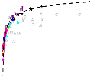
  $k-\epsilon$ models as reported in Wilcox Reference Wilcox2006). Nevertheless, as found in direct numerical simulations (DNS) (Spalart Reference Spalart1988; Iwamoto, Suzuki & Kasagi Reference Iwamoto, Suzuki and Kasagi2002; Hoyas & Jimenez Reference Hoyas and Jimenez2006; Wu & Moin Reference Wu and Moin2008; Schlatter et al. Reference Schlatter, Örlü, Li, Brethouwer, Fransson, Johansson, Alfredsson and Henningson2009; Sillero, Jimenez & Moser Reference Sillero, Jimenez and Moser2013; Ahn et al. Reference Ahn, Lee, Lee, Kang and Sung2015; Lee & Moser Reference Lee and Moser2015; Yamamoto & Tsuji Reference Yamamoto and Tsuji2018) as well as laboratory experiments (Sreenivasan Reference Sreenivasan1989; DeGraaff & Eaton Reference DeGraaff and Eaton2000; Örlü Reference Örlü2009; Hultmark et al. Reference Hultmark, Vallikivi, Bailey and Smits2012; Vincenti et al. Reference Vincenti, Klewicki, Morrill-Winter, White and Wosnik2013; Marusic et al. Reference Marusic, Chauhan, Kulandaivelu and Hutchins2015; Vallikivi, Ganapathisubramani & Smits Reference Vallikivi, Ganapathisubramani and Smits2015; Willert et al. Reference Willert, Soria, Stanislas, Klinner, Amili, Eisfelder, Cuvier, Bellani, Fiorini and Talamelli2017; Samie et al. Reference Samie, Marusic, Hutchins, Fu, Fan, Hultmark and Smits2018), the streamwise turbulence intensity, the dominant contributor to turbulent fluctuations, exhibits a notable dependence on the Reynolds number. As summarized in figure 1, the normalized peak value,
  $\overline {u'u'}^+_p$, exhibits an almost 150 % growth for
  $Re$ of the order
  $10^2$ to
  $10^4$; here,
  $Re$ is the Reynolds number based on
  ${u_\tau } = {\tau _w}^{1/2}$ and the flow thickness is
  $\delta$; here and elsewhere, superscript
  $+$ indicates the normalization by wall variables
  ${u_\tau }$ and
  $\nu$, and the overbar indicates the time average. This feature cannot be explained away by stating that the flow has not reached a fully developed state, and so triggers a challenge for the classical wall-scaling for turbulent intensity, particularly for high-
 $Re$ predictions.

FIG. 1. Reynolds number dependence of the near-wall streamwise turbulence intensity peak  $\overline {u'u'}^+_p$ normalized by friction velocity square
  $u^2_\tau$. Solid line indicates the logarithmic growth of (1.1) given by Marusic, Baars & Hutchins (Reference Marusic, Baars and Hutchins2017); dashed line is the defect power-law growth, (4.2), newly obtained in this paper, as will be explained in the text. Symbols are for data from channel, pipe and TBL: solid symbols are from DNS and the rest from experiments. References to the data are presented in the panel.
For the last two decades, considerable effort has been devoted to understanding this growth, almost all of which (see Marusic, Baars & Hutchins (Reference Marusic, Baars and Hutchins2017) and references therein) proposes the logarithmic form
 \begin{equation} \overline{u'u'}^+_p=A\ln Re + B, \end{equation}
where A and B are constants. The reason for this logarithmic growth, according to Marusic et al. (Reference Marusic, Baars and Hutchins2017), is the inner--outer interaction between near wall and outer flow eddies, captured in good measure by the attached-eddy model of Townsend. The inner--outer interaction can also be understood from the perspective of mixed scaling (Sreenivasan Reference Sreenivasan1989; DeGraaff & Eaton Reference DeGraaff and Eaton2000), according to which turbulence intensity scales as the geometric mean of  $u_\tau$ and
  $\bar {u}_e$, where
  $\bar {u}_e$ is the centreline velocity of channel and pipe, or the free-stream velocity of the turbulent boundary layer (TBL). We thus have
 \begin{equation} \overline{u'u'}^+_p \equiv \frac{\overline{u'u'}_p}{u^2_\tau}=\frac{\overline{u'u'}_p}{u_\tau \bar{u}_e}\frac{\bar{u}_e}{u_\tau}\propto\frac{\bar{u}_e}{u_\tau}\propto \ln Re, \end{equation}
where, in the last step, we have used the well-known result from the log-law for the mean velocity  $\bar {u}$, which gives
  $\bar {u}_e/u_\tau \propto \ln Re$. With the two fitting parameters
  $A=0.63$ and
  $B=3.80$ given in Marusic et al. (Reference Marusic, Baars and Hutchins2017), (1.1) represents the data quite well, as the solid line in figure 1 shows. If it continues to remain valid for very high
  $Re$, the logarithmic growth indicates the failure of the wall-scaling for turbulence intensity. The dashed line is the alternative result derived here. The rest of the paper is concerned with its derivation and interpretation.
Before proceeding further, we should note that Monkewitz & Nagib (Reference Monkewitz and Nagib2015) have questioned the mixed scaling for  $\overline {u'u'}$ in TBL. They found that the mixed scaling is ruled out for the logarithmic mean velocity profile if one assumes that the Reynolds normal stress term
  ${\partial _x}\overline {u'u'}$ is of the same order as the mean convective terms
  $\bar {u}{\partial _x}\bar {u} + \bar {v}{\partial _y}\bar {u}$ (where v is the wall-normal velocity). This argument leads to the classical viscous scaling for near-wall
  $\overline {u'u'}$ and implies a finite near-wall peak as
  $Re\rightarrow \infty$. By examining the available data, these authors further suggested that the asymptotic peak value is approximately 22 and the departure from this asymptote has the form
  $1/\ln (Re)$, i.e.
  $\overline {u'u'} _p^ + \approx 22 \text {--}340/\bar {u}_e^ +$. However, their analysis does not necessarily exclude mixed scaling if
  ${\partial _x}\overline {u'u'}$ scales differently (e.g. as the residue between the derivatives of viscous shear and Reynolds shear stress) – without causing a problem for the momentum balance. Moreover, as noted by Monkewitz & Nagib (Reference Monkewitz and Nagib2015), their analysis is restricted to TBL but not applicable to channel and pipe flows, as the latter two have no
  ${\partial _x}\overline {u'u'}$ term in the mean momentum equation. Yet, all three flows show a similar
  $Re$-dependence of
  $\overline {u'u'}^+_p$. Therefore, mere order of magnitude analysis cannot provide a conclusive answer for the scaling of
  $\overline {u'u'}$, and a common explanation on the
  $Re$-dependence of peak value for the three flows is still desired.
2 A plausible argument against the continued growth of  $\overline {u'u'}^+_p$

We now demonstrate that any sustained growth of  $\overline {u'u'} _p^ +$, such as the logarithmic growth of (1.2), comes with a difficulty. The balance equation of
  $\overline {u'u'}$, derived from Navier–Stokes equations, presented here in a general form for the channel, pipe and TBL, reads as
 \begin{equation} S^+W^++\mathcal{D}^+-\epsilon^+= \mathcal{N}^+, \end{equation}
where the turbulent production  $\mathcal {P}^+=S^+W^+$ is the product of the mean shear
  $S^+={\partial {\bar {u}^+}}/{\partial {y^+}}$ and Reynolds shear stress
  $W^+=-\overline {u'v'}^+$, turbulent diffusion is given by
  $\mathcal {D}^+=\frac {1}{2}({\partial ^2}/{\partial y^{+2}}){\overline {u'^2}^+}$, the dissipation by
  $\epsilon ^+=\overline {|\boldsymbol {\nabla }{u'}|^+}^2$ and
  $\mathcal {N}^+$ includes the transport term and nonlinear correlation of pressure and velocity fluctuations. Very close to the wall, the leading order balance in (2.1) is between diffusion and dissipation (Chen, Hussain & She Reference Chen, Hussain and She2018), this being exact at the wall so that
 \begin{equation} \mathcal{D}^+_w=\epsilon^+_w, \end{equation}
with the subscript  $w$ indicating conditions at the wall. By the Taylor expansion of
  $\overline {u'u'}^+$, i.e.
  $\overline {u'u'}^+= \mathcal {D}^+_w y^{+2}+\,$high order terms, one can estimate the order of the peak value located at
  $y^+_p$ as
 \begin{equation} \overline{u'u'}^+_p\sim\mathcal{D}^+_w y^{+2}_{p}= \epsilon^+_w y^{+2}_{p} \end{equation}
(where the ‘ $\sim$’ sign represents an estimate from the expansion and the ‘
 $=$’ sign results from (2.2)). To understand the behaviour of this equation as
  $Re \to \infty$, note that all available evidence (see e.g. Sreenivasan Reference Sreenivasan1989; Metzger & Klewicki Reference Metzger and Klewicki2001; Lee & Moser Reference Lee and Moser2015) suggests that the position
  $y_p^+$ of
  $\overline {u'u'}^+_p$ is remarkably independent of the Reynolds number. Thus, (2.3) should be a reasonable order of magnitude estimate in the large-
 $Re$ limit. If so, any boundless increase of the left-hand side of (2.3) with respect to
  $Re$ would mean that
  $\epsilon ^+_w \to \infty$, which is an implausible result.
The most important reason for expecting  $\epsilon ^+_w$ to be bounded is as follows. The energy production essentially balances dissipation in the region of peak production. Therefore, an infinite dissipation would imply an infinite production but it is well known (Sreenivasan Reference Sreenivasan1989; Chen et al. Reference Chen, Hussain and She2018) that, in these units, the maximum production is bounded by
  $1/4$. To see this, note that the mean momentum balance near the wall approximates to
 \begin{equation} S^++W^+ \approx1, \end{equation}
which yields the maximum for  $S^+W^+$ when
  $S^+=W^+=1/2$ (around
  $y^+\approx 12$ as summarized, e.g. in Sreenivasan (Reference Sreenivasan1989), She, Chen & Hussain (Reference She, Chen and Hussain2017) and Cantwell (Reference Cantwell2019). That is,
 \begin{equation} \mathcal{P}^+_{\infty}=(S^+W^+)_{max} =(1/2)*(1/2)={1/4}. \end{equation}
This bound on the production argues against a boundless increase of the wall dissipation even in the limit of infinite Reynolds number. We are thus driven to find an alternative scaling rather than persist with the logarithmic growth of the peak in the streamwise velocity fluctuation.
3 Scaling of the dissipation rate at the wall
If every term in (2.1) is surmised to be bounded, we define the amount of dissipation rate that departs from its limiting value  $\epsilon ^+_\infty =1/4$ as
 \begin{equation} \epsilon^+_d=\epsilon^+_\infty-\epsilon^+_w=1/4-\epsilon^+_w. \end{equation}
The quantity  $\epsilon ^+_d= \epsilon _d/ (u^4_\tau /\nu )$, which is the ‘defect’ dissipation that falls short of the asymptotic maximum of 1/4, is relevant to our analysis of how the dissipation near the wall asymptotes to the limit. A similar defect quantity, defined for the maximum Reynolds shear stress in Chen, Hussain & She (Reference Chen, Hussain and She2019), reveals a non-universal scaling transition of momentum transfer among channel, pipe and TBL flows.
If the energy dissipation near the wall were to follow the wall-law, as might be expected for infinitely large Reynolds number, it would be given by  $u_\tau ^2/(\nu /u_\tau ^2) = u_\tau ^4/\nu$. (One can also obtain this result, as did Monkewitz & Nagib (Reference Monkewitz and Nagib2015), by integrating the suitably normalized form of Kolmogorov's
  $-5/3$ spectrum for
  $\overline {u'u'}$.) At any finite Reynolds number, however, the energy dissipation near the wall falls short of
  $u_\tau ^4/\nu$ because some of the energy produced there is transmitted to the outer layer without getting dissipated locally, and this happens presumably over a typical time scale that is smaller than
  $\delta /u_\tau$ but larger than
  $\nu /u_\tau ^2$, as suggested by past studies of turbulent bursting (Rao, Narasimha & Narayanan Reference Rao, Narasimha and Narayanan1971). One might regard this time scale as the one that the outer layer imposes on the inner layer – small for the outer layer but large for the inner layer. A conjecture is that this scale is given by
  $\eta _o/u_\tau$, where
  $u_\tau$ is the typical velocity scale for wall flows while the length scale
  $\eta _o$ is the key assumption, proposed as the smallest (Kolomogorov) length for the outer region given by
 \begin{equation} {\eta _o} = {\nu ^{3/4}}/\epsilon _o^{1/4}; \quad\epsilon _o = u_\tau ^3/\delta, \end{equation}
where the subscript ‘o’ refers to the outer region of the wall flow ( ${\epsilon}_{o}$ is the outer dissipation scale). Accordingly, we have
 \begin{equation} \epsilon_d \sim u_\tau ^3/{\eta _o} \sim \varepsilon _o Re ^{3/4}, \end{equation}
where we used (3.2a,b) (in this section, the sign ‘ $\sim$’ means ‘scales as’). Putting (3.3) in wall units, we get
 \begin{equation} \epsilon^+_d =\epsilon_d/(u^4_\tau/\nu)\sim\epsilon_o Re^{3/4}/(u^4_\tau/\nu) \sim Re ^{-1/4}, \end{equation}
from which it follows that
 \begin{equation} \epsilon^+_w=1/4-\epsilon^+_d =1/4-\beta/ Re^{1/4}. \end{equation}
Clearly  $\epsilon ^+_d$ decreases with increasing
  $Re$, and (3.5) shows how
  $\epsilon ^+_w$ approaches its upper limit of a 1/4. In figure 2(a), we display the defect dissipation rate versus
  $Re$ and observe an excellent
  $-1/4$ power, as given by (3.5). The only fitting parameter is the proportionality coefficient
  $\beta \approx 0.42$, estimated from the DNS data at
  $Re=1000$, which is the middle of the range covered here. Note that the time scale
  $\eta _o/u_\tau$ is proposed to be the same for channel, pipe and TBL flows, while the proportionality coefficient
  $\beta$ – attributed to the outer flow influence – may be flow dependent. The geometry effect on the near-wall quantities, as well as uncertainty on the wall-dissipation data (through direct and indirect estimation), are important and deserve a thorough investigation in the future, and are not discussed here. Moreover, figure 2(b) compares (3.5) with the logarithmic fit by Tardu (Reference Tardu2017), i.e.
  $\epsilon ^+_w=0.02\ln Re+0.035$, and shows that the present fit describes the data better.

FIG. 2. (a) The defect dissipation rate at the wall from its upper bound of 1/4 showing an excellent  $Re^{-1/4}$ fit as predicted by (3.5), dashed line. (b) Wall-dissipation rate varying with
  $Re$ in close agreement with (3.5), dashed line; also included for comparison is the logarithmic fitting by Tardu (Reference Tardu2017), i.e.
  $0.02\ln Re+0.035$, solid line. Symbols are from DNS data in channel flows at different values of
  $Re$. For the data legend, see figure 1.
It should be stressed that (3.3) contains specific physics which can be tested more directly than is done here. Essentially, the physics is that the smallest scale in the outer layer, given by its characteristic Kolmogorov scale, is the largest scale that the wall layer sees. Thus, the effective range of scales available to the energetics of the wall layer ranges between  $\eta _0$ and local
  $\eta$, with their ratio given by
  $Re^{1/4}$.
4 Scaling of streamwise turbulence intensity peak
Substituting (3.5) into (2.3) yields
 \begin{equation} \overline{u'u'}^+_p\sim \mathcal{D}^+_w y^{+2}_p = \epsilon^+_w y^{+2}_p=(1/4-\beta \,Re^{-1/4})y^{+2}_p, \end{equation}
which can be rewritten as
 \begin{equation} \overline{u'u'}^+_p=\alpha(1/4-\beta\, Re^{-1/4})=\overline{u'u'}^+_\infty-\gamma\,Re ^{-1/4}, \end{equation}
where  $\overline {u'u'}^+_\infty =\alpha /4$ (
 $\alpha$ is a proportional coefficient) and
  $\gamma =\alpha \beta$. At the typical Reynolds number of 1000,
  $\overline {u'u'}^+_p\approx 8.1$ from DNS data (Lee & Moser Reference Lee and Moser2015); taken together with
  $\beta \approx 0.42$ shown in figure 2, we get
  $\alpha \approx 46$ from (4.2). (It will be shown by a different reasoning in § 5 that
  $\alpha$ is close to
  $y^{+2}_p/4\approx 49$.) We also have
  $\gamma \approx 19.32$ and
  $\overline {u'u'}^+_\infty = \alpha /4\approx 11.5$, this being our predicted asymptotic peak value as
  $Re\rightarrow \infty$.
Validations of (4.2) with  $\alpha =46$ and
  $\beta =0.42$ are shown in figures 1 and 3. For comparison, we have collected data of three wall flows from both DNS and experimental measurements. Not only are the DNS data with the highest
  $Re$ reported in literature included –
  $Re$ up to
  $8000$ for channel (Yamamoto & Tsuji Reference Yamamoto and Tsuji2018), 3000 for pipe (Ahn et al. Reference Ahn, Lee, Lee, Kang and Sung2015) and 2000 for TBL (Sillero et al. Reference Sillero, Jimenez and Moser2013) – but also included are other DNS data of channels (Iwamoto et al. Reference Iwamoto, Suzuki and Kasagi2002; Hoyas & Jimenez Reference Hoyas and Jimenez2006; Lee & Moser Reference Lee and Moser2015), pipes (Wu & Moin Reference Wu and Moin2008) and TBL (Spalart Reference Spalart1988; Schlatter et al. Reference Schlatter, Örlü, Li, Brethouwer, Fransson, Johansson, Alfredsson and Henningson2009). Experimental data for pipes and TBL from worldwide facilities (DeGraaff & Eaton Reference DeGraaff and Eaton2000; Örlü Reference Örlü2009; Hultmark et al. Reference Hultmark, Vallikivi, Bailey and Smits2012; Vincenti et al. Reference Vincenti, Klewicki, Morrill-Winter, White and Wosnik2013; Marusic et al. Reference Marusic, Chauhan, Kulandaivelu and Hutchins2015; Vallikivi et al. Reference Vallikivi, Ganapathisubramani and Smits2015; Willert et al. Reference Willert, Soria, Stanislas, Klinner, Amili, Eisfelder, Cuvier, Bellani, Fiorini and Talamelli2017; Samie et al. Reference Samie, Marusic, Hutchins, Fu, Fan, Hultmark and Smits2018) are collected as well. These data cover more than two decades in
  $Re$, offering a good benchmark for validating the proposed scaling law. Note that differing from Marusic et al. (Reference Marusic, Baars and Hutchins2017) where
  $Re$ of TBL was defined by the thickness obtained via mean velocity log-law fitting (see Marusic et al. (Reference Marusic, Chauhan, Kulandaivelu and Hutchins2015) for details), we use
  $\delta _{99}$ as the boundary layer thickness and hence
  $Re=u_\tau \delta _{99}/\nu$ for TBL flows. Also, data of Vincenti et al. (Reference Vincenti, Klewicki, Morrill-Winter, White and Wosnik2013) are not taken from any plot in Marusic et al. (Reference Marusic, Baars and Hutchins2017) but from original data authors.

FIG. 3. Streamwise turbulence intensity peak versus the logarithm of  $Re$. Panel (a) compares data with (1.1) given by Marusic, Baars & Hutchins (Reference Marusic, Baars and Hutchins2017), solid line; Panel (b) compares the same data with (4.2), dashed line. Data are the same as in figure 1.
As shown in figure 1, (4.2) agrees closely with data. Experimental data show considerable scatter, which is not surprising because the accurate measurement of  $\overline {u'u'}$ is still a challenging task due to limited resolution in experimental techniques (see discussions in Örlü & Alfredsson Reference Örlü and Alfredsson2013; Samie et al. Reference Samie, Marusic, Hutchins, Fu, Fan, Hultmark and Smits2018). The lack of resolution is more grievous at larger
  $Re$, which may cause the apparent saturation judged from the largest
  $Re$ measurements in Hultmark et al. (Reference Hultmark, Vallikivi, Bailey and Smits2012), Willert et al. (Reference Willert, Soria, Stanislas, Klinner, Amili, Eisfelder, Cuvier, Bellani, Fiorini and Talamelli2017) and Vallikivi et al. (Reference Vallikivi, Ganapathisubramani and Smits2015), represented by the grey symbols in figure 1. Except for these data, all the others display a clear monotonic increase with
  $Re$, well captured by (4.2). Further, the very recent measurements by Princeton group (Smits Reference Smits2019) have started to exhibit a
  $Re$-dependent increase of the near-wall peak.
A few further comments are useful. Figure 3 shows that the data depart from (1.1) towards small  $Re$. Considering the fact that parameters
  $A=0.63$ and
  $B=3.80$ in Marusic et al. (Reference Marusic, Baars and Hutchins2017) are chosen for the best fit of high-
 $Re$ data, they can indeed be readjusted to reduce the departure at small
  $Re$ but this would ruin the agreement with higher
  $Re$. What is clear is that the data from
  $Re=500$ to
  $2000$ exhibit a steeper slope (i.e.
  $A\approx 0.75$) than data from
  $Re=2000$ to
  $20\,000$ (with
  $A\approx 0.63$), and an overall concave trend might be inferred. This feature is depicted well by (4.2), which agrees with the data. It is of interest to note that, in the atmospheric surface layer measured over the salt flats of the Great Salt Lake Desert, Metzger & Klewicki (Reference Metzger and Klewicki2001) observed that
  $\overline {u'u'}^+_p$ occurs around 13.4 at
  $Re=9\times 10^5$, with the uncertainty between 11.6 and 15.2. The lower bound is consistent with our estimation of
  $11.5$ from (4.2). Therefore, we might reasonably surmise that the formula (4.2) presents a universal scaling law for the three flows of channel, pipe and TBL, with the advantage of a finite limiting value as
  $Re$ increases.
5 Discussion
An issue to clarify is why (4.2) works well for the peak magnitude without demanding anything specifically about the non-monotonicity of  $\overline {u'u'}^+$. A superficial view is that the deviation of the inner
  $\overline {u'u'}^+$ profile from the expansion (2.3) or (4.1) is not large at the peak location
  $y^+_p$. The underlying reason is that the higher-order terms beyond the Taylor expansion are now accounted for by the proportional coefficient
  $\alpha /y^{+2}_p\approx 0.23$ – close to
  $1/4$ – in (4.2). To see this, we develop the following analysis.
First, due to the no-slip wall condition, Reynolds shear stress has the expansion
 \begin{equation} -\overline{u'v'}\propto y^3,\quad or \quad-\overline{u'v'}^+\approx C y^{+3}, \end{equation}
where  $C$ is a proportionality coefficient. In Chen et al. (Reference Chen, Hussain and She2018), a higher-order expression of
  $\overline {u'v'}^+$ was obtained by introducing the length function
  $\ell =\sqrt {-\overline {u'v'}^+}/(\textrm {d}\bar {u}^+/{\textrm {d} y}^+)$. Accordingly, the momentum equation (2.4) can be written as
 \begin{equation} -\overline{u'v'}^++\sqrt{-\overline{u'v'}^+}/\ell^+\approx1. \end{equation}
Considering only the leading order balance of (5.2), i.e.  $\sqrt {-\overline {u'v'}^+}/\ell ^+\approx 1$, one has
 \begin{equation} \ell^+\approx C^{1/2} y^{+3/2}. \end{equation}
On the other hand, with all terms in (2.4) included, (5.2) leads to the analytical expression
 \begin{equation} -\overline{u'v'}^+=1-\frac{2}{1+\sqrt{1+4\ell^{+2}}}. \end{equation}
Interestingly, the substitution of (5.3) in (5.4) yields
 \begin{equation} -\overline{u'v'}^+\approx1-\frac{2}{1+\sqrt{1+4Cy^{+3}}}. \end{equation}
If  $\overline {u'u'}^+ \sim \mathcal {D}^+_w y^{+2} = \mathcal {\epsilon }^+_w y^{+2}$, one gets that
  $-\overline {u'u'}^+/\overline {u'v'}^+\approx C'/{y^+}$ with
  $C'\approx {\mathcal {\epsilon }^+_w/C}$, and from (5.5) we have
 \begin{equation} \overline{u'u'}^+\approx\frac{C'}{y^+}\left[1-\frac{2}{1+\sqrt{1+4Cy^{+3}}}\right]. \end{equation}
As verified in Chen et al. (Reference Chen, Hussain and She2018), the above approximation depicts a non-monotonic variation of  $\overline {u'u'}$ and agrees well with data from the wall up to
  $y^+\approx 30$, well beyond the near-wall peak. Hence, it is reasonable to use (5.6) to estimate the peak of
  $\overline {u'u'}^+$ by setting
  $\textrm {d}\overline {u'u'}^+/{\textrm {d} y}^+=0$. Equation (5.6) then leads to
 \begin{equation} y^+_p\approx 2^{{1}/{3}}C^{-{1}/{3}}; \end{equation}
substituting (5.7) into (5.6) one obtains the peak magnitude to be
 \begin{equation} \overline{u'u'}^+_p\approx {2^{-{4}/{3}}}C^{{-2}/{3}} {{\epsilon}^+_w}\approx (y^{+2}_p/4) {{\epsilon}^+_w}. \end{equation}
Comparing (5.8) with (4.2), we obtain the estimates
 \begin{equation} \alpha\approx y^{+2}_p/4;\quad\overline{u'u'}^+_\infty=\alpha/4\approx y_p^{+2}/16. \end{equation}
This result explains that in (4.1) and (4.2), the anticipated higher-order corrections to the Taylor expansion are now accounted for by the proportional coefficient  $\alpha /y^{+2}_p\approx 1/4$. The new physics involved here are the Reynolds shear stress in (5.5) and the invariance of the ratio between
  $\overline {u'u'}^+$ and
  $\overline {u'v'}^+$ – both verified in Chen et al. (Reference Chen, Hussain and She2018). With
  $y^+_p=14$, we have
  $\alpha \approx 49$ from (5.9a,b), and hence
  $\overline {u'u'}^+_\infty \approx 12.2$, very close to
  $\alpha \approx 46$ and
  $\overline {u'u'}^+_\infty = \alpha /4\approx 11.5$ used for data comparisons in figures 1 and 3. The estimates again demonstrate that the peak magnitude is bounded by a finite value of
  $y^+_p$. Note that (5.9a,b) also indicates that a 10 % uncertainty of
  $y_p^+$ results in a
  $20\,\%$ uncertainty of the magnitude. Note also that
  $y_p^+\approx 14$ at
  $Re=300$ from a DNS channel (Iwamoto et al. Reference Iwamoto, Suzuki and Kasagi2002), almost the same as
  $y_p^+\approx 15$ at
  $Re=9\times 10^5$ from the atmospheric surface layer observation by Metzger & Klewicki (Reference Metzger and Klewicki2001), so the
  $Re$-variation of
  $y^+_p$ is quite weak – if it exists at all. It should be mentioned, however, that the atmospheric surface layer data in Metzger et al. (Reference Metzger, Klewicki, Bradshaw and Sadr2001) leave open the possibility that
  $y_p^+$ may extend beyond
  $23$.
$23$.
6 Conclusion
The main point of this paper is that the asymptotic value of  $1/4$ (scaled by
  $u^4_\tau /\nu$) for the maximum turbulent production provides a constraint on the dissipation rate and turbulent diffusion at the wall. The new defect law,
  $1/4-\epsilon ^+_w\propto Re^{-1/4}$, indicates that the dissipation rate in the wall region, caused by the small eddies in the viscous range, is influenced by the outer layer directly. This, in turn, leads to a similar defect power-law for the streamwise turbulence intensity peak, i.e.
  $\overline {u'u'}^+_\infty -\overline {u'u'}^+_p\propto Re^{-1/4}$, showing a finite turbulent intensity peak near the wall as
  $Re \to \infty$. We believe that this is a powerful statement, whose qualitative physics is that the smallest scales of the outer layer form the largest scales of the wall layer.
Compared to the logarithmic growth, the present scaling proposals present a similarly good, if not better, description of data for the  $Re$ domain currently covered for channel, pipe and TBL flows. At the minimum, it presents an alternative formulation which successfully agrees with the data. Though close to each other at the current
  $Re$ domain, the most important difference occurs as
  $Re\rightarrow \infty$. While the logarithmic scaling indicates a divergent near-wall peak, the present results predict a finite limit and lend support to the classical wall-scaling for turbulence intensity at asymptotically high Reynolds numbers.
Acknowledgements
We are grateful to all the authors cited in figure 1 (particularly J. Klewicki) for making their data available, to I. Marusic for useful correspondence and to the anonymous referees whose comments improved the paper. X.C. appreciates beneficial discussions with J.C. Vassilicos and J.P. Laval and the funding support by the grants KG16045601 (BUAA) and KZ73030006 (NSFC).
Declaration of interests
The authors report no conflict of interest.


