


1. Introduction
Coherent structures in complex flows have been the focus of much research interest, with considerable effort devoted specifically to the study of coherent structures in turbulence (Sirovich Reference Sirovich1987; Waleffe Reference Waleffe2001; Neamtu-Halic et al. Reference Neamtu-Halic, Krug, Mollicone, Van Reeuwijk, Haller and Holzner2020). Although coherent structures play an important role in the transport and mixing of fluid particles, their physical description is not well understood. Various definitions of coherent structures have been proposed from different perspectives. Haller & Yuan (Reference Haller and Yuan2000) cite example definitions of coherent structures as collections of fluid particles with distinct statistical features (Elhmaïdi, Provenzale & Babiano Reference Elhmaïdi, Provenzale and Babiano1993), energetically dominant recurrent patterns (Holmes, Lumley & Berkooz Reference Holmes, Lumley and Berkooz1996) and concentrated vorticity zones that maintain their identity over long periods of time (Provenzale Reference Provenzale1999). From an analytical point of view, methods for extracting coherent structures may be divided into Eulerian and Lagrangian approaches.
Eulerian approaches capture coherent structures by examining the instantaneous distribution of different scalar fields (such as vorticity, kinetic energy, strain, etc.) in the flow field. Such approaches are widely applied to vortex identification. Commonly used analysis methods include the Okubo–Weiss criterion (Okubo Reference Okubo1970; Weiss Reference Weiss1991),  $Q$-criterion (Hunt, Wray & Moin Reference Hunt, Wray and Moin1988),
  $\varDelta$-criterion (Chong, Perry & Cantwell Reference Chong, Perry and Cantwell1990) and
  $\lambda _2$-criterion (Jeong & Hussein Reference Jeong and Hussein1995). Although these methods effectively frame coherent features of the instantaneous velocity field, a threshold value has to be set artificially in order to properly capture the vortex structure(s). In an unsteady flow, coherently evolving velocity features tend to differ substantially from coherently moving fluid parcels, and so Eulerian approaches experience difficulty in determining the true coherent structures in the flow. Most Eulerian vortex identification approaches lack objectivity (i.e. frame independence), which means that they cannot remain invariant with respect to time-dependent rotation and translation of the reference frame. However, there exist a few notable exceptions, such as instantaneous vorticity deviation (Haller et al. Reference Haller, Hadjighasem, Farazmand and Huhn2016), the instantaneous version of the finite-time Lyapunov exponent (FTLE) field (Nolan, Serra & Ross Reference Nolan, Serra and Ross2020) and objective Eulerian coherent structures (Serra & Haller Reference Serra and Haller2016).
Unlike Eulerian approaches, the Lagrangian approach investigates advection and diffusion processes by regarding the flow field as a dynamical system composed entirely of fluid particles. More precisely, the Lagrangian approach determines the most influential coherent structures in a flow by tracing the separation of fluid particles over a finite-time interval of interest. With the development of chaos theory, it has been discovered that the trajectory of an individual fluid particle in a complex flow is often highly sensitive to small changes in the particle's initial condition. However, as pointed out by Haller (Reference Haller2015), ‘behind complex and sensitive tracer patterns … there exists a robust skeleton of material surfaces, Lagrangian coherent structures, shaping those patterns’. Haller described Lagrangian coherent structures (LCSs) as ‘the most repelling, attracting, and shearing material surfaces that form the skeleton of Lagrangian particle dynamics’. In recent decades, LCSs have proved to be of great use in analysing Lagrangian coherence in finite-time dynamical systems.
Methods by which to analyse Lagrangian coherence are usually divided into two broad categories: diagnostic and analytical (Hadjighasem et al. Reference Hadjighasem, Farazmand, Blazevski, Froyland and Haller2017). Diagnostic methods provide a scalar field whose features are expected to reveal coherent structures based on certain geometric or physical parameters. Most of these methods do not strictly define the coherent structures, nor do they establish the precise mathematical relationship between the geometric characteristics of the scalar fields and the coherent structures. Therefore, even for some simple flows, these approaches may result in false positives and negatives. For instance, without additional mathematical criteria, FTLE struggles to differentiate between repelling and shearing effects (Branicki & Wiggins Reference Branicki and Wiggins2010). On the other hand, diagnostic methods are still widely used, being easy to calculate and providing a rapid visualization of the unknown flow field that is useful for preliminary understanding. Analytical methods define coherent structures as precise solutions of mathematically formulated coherence principles. A recent advance in geodesic LCS theory seeks an LCS as a stationary curve of the Lagrangian strain or shear functional computed along material lines (Haller & Beron-Vera Reference Haller and Beron-Vera2012, Reference Haller and Beron-Vera2013; Farazmand, Blazevski & Haller Reference Farazmand, Blazevski and Haller2014). The foregoing variational method reveals LCSs to be null geodesics of appropriate strain tensor fields computed from the deformation field. Geodesic LCS theory extracts transport barriers as material lines whose functions are similar to those in classical dynamical systems (e.g. stable and unstable manifolds, shear jets and Kolmogorov–Arnold–Moser curves), and partitions the flow geometrically into regions with distinct properties.
The methods used to extract LCSs in the present paper depend solely on frame-invariant tensor fields and, hence, remain the same in translating and rotating frames. Moreover, they possess the ability to define structure boundaries without relying on a preselected threshold. A further advantage is their insensitivity to short-term anomalies in the velocity field. Nevertheless, Lagrangian quantities can be computationally expensive to determine, because a large number of trajectories are involved in the integration of fluid particles.
As an objective tool, LCS methods have been applied to various flows in order to extract coherent structures. For example, Cardwell & Mohseni (Reference Cardwell and Mohseni2007) used LCS analysis to study boundary layer reattachment and the shedding of wake vortices for numerical simulations of a two-dimensional airfoil under low-Reynolds-number conditions. They found that the LCS approach can capture more detail than Eulerian methods, with the formation, shedding and rupture of vortices more obvious. Peng & Dabiri (Reference Peng and Dabiri2009) applied the LCS method to a planktonic predator–prey system, and identified the region where moon jellyfish (Aurelia aurita) captures its prey. This enabled analysis of the influence of parameters such as prey size, escape ability and predator perception on the interaction between prey and predator. Hadjighasem & Haller (Reference Hadjighasem and Haller2016) processed video images captured by NASA's Cassini space mission, and extracted elliptic LCSs and parabolic LCSs concerning Jupiter's great red spot and atmospheric jet stream using geodesic theory. Suara et al. (Reference Suara, Khanarmuei, Ghosh, Yu, Zhang, Soomere and Brown2020) used LCS to study the source and destination of marine debris in Moreton Bay on the southeast coast of Queensland, Australia, and found that islands play an important role in preventing material transport and mixing in the bay.
Flow past a backward-facing step (BFS) is a typical benchmark separation flow problem with rich flow physics that incorporates shear layer separation and reattachment together with primary and secondary recirculation regions in the lee of the step. Engineering applications of BFS flow include diffusers, combustors, ducts and channels with sudden expansions encountered in internal flow systems, and surface furrows and ridges on airfoils and vehicles in external flows. Owing to the geometrical simplicity of the BFS, many theoretical and experimental studies have been undertaken (Brown & Roshko Reference Brown and Roshko1974; Armaly et al. Reference Armaly, Durst, Pereira and Schönung1983; Le, Moin & Kim Reference Le, Moin and Kim1997; Nadge & Govardhan Reference Nadge and Govardhan2014). Perhaps surprisingly, there is considerable disparity in the literature on BFS flows even with regard to the time-averaged reattachment length. The hidden mechanisms behind BFS flow remain to be fully investigated, one of which is the formation and development of coherent structures. To date it has been established that coherent structures play an important role in the dynamics of the separated shear layer, contributing significantly to flapping movements and high-order harmonic oscillations (Ma & Schröder Reference Ma and Schröder2017). An improved knowledge of the hidden nonlinear dynamics of coherent structures might contribute to the creation of an effective solution to the flow separation control problem. Although Eulerian approaches for identifying coherent structures have long been utilized (Neto et al. Reference Neto, Grand, Métais and Lesieur1993; Hu, Wang & Fu Reference Hu, Wang and Fu2016), Lagrangian approaches have received less attention with their application limited to FTLE (Sampath, Mathur & Chakravarthy Reference Sampath, Mathur and Chakravarthy2016; Yang et al. Reference Yang, He, Shen and Luo2021).
In this paper we apply two types of diagnostic method (the FTLE and polar rotation angle (PRA)) and an analytical method (geodesic LCS theory) to detect LCSs in a BFS flow whose configuration is consistent with that studied in the combustion experiment conducted by Pitz & Daily (Reference Pitz and Daily1983). Complementary qualitative and quantitative analyses are used to uncover the underlying structures within flow past a BFS by employing both categories of LCS-detection methods. Here, we idealise the flow past a BFS as a two-dimensional problem in the plane. We therefore neglect gravitational acceleration, which is reasonable for gas flow through a duct where the speed of sound in the fluid is much larger than the flow speed.
2. Methods
2.1. Diagnostic methods: FTLE and PRA
Consider a two-dimensional unsteady flow velocity field,
 \begin{equation} \dot{\boldsymbol{x}}=\boldsymbol{u}(t, \boldsymbol{x}), \quad \boldsymbol{x} \in U \subset \mathbb{R}^{2}, \quad t \in\left[t_{0}, t_{1}\right], \end{equation}
where  $\boldsymbol {x}$ is the distance vector in cartesian coordinates,
  $\boldsymbol {u}$ is the vector of velocity components,
  $t$ is time,
  $U$ is the flow domain,
  $t_{0}$ is start time and
  $t_{1}$ is end time. Solutions of this ordinary differential equation (ODE) define the flow map,
 \begin{equation} \mathcal{F}_{t_{0}}^{t}\left(\boldsymbol{x}_{0}\right):=\boldsymbol{x}\left(t ; t_{0}, \boldsymbol{x}_{0}\right), \end{equation}
which states that a fluid particle whose initial position is  $\boldsymbol {x}_0$ at time
  $t_0$ is mapped onto
  $\boldsymbol {x}(t; t_0, \boldsymbol {x}_0)$ at time
  $t$ by the flow map
  $\mathcal {F}$. Consider a material line
  $\gamma$ of initial condition
  $\gamma (t_0)$ whose position
  $\gamma (t)$ at time
  $t$ satisfies
 \begin{equation} \gamma(t) = \mathcal{F}^{t}_{t_0}(\gamma(t_0)). \end{equation}
To assess the influence of specific material lines on trajectories, we utilize a classical measure of flow deformation, the right Cauchy–Green strain tensor
 \begin{equation} \boldsymbol{\mathsf{C}}^{t}_{t_0}(\boldsymbol{x}_0) = \left[\boldsymbol{\nabla} \mathcal{F}^{t}_{t_0}(\boldsymbol{x}_0) \right]^{\mathrm{T}} \boldsymbol{\nabla} \mathcal{F}^{t}_{t_0}(\boldsymbol{x}_0), \end{equation}
where  $\boldsymbol {\nabla }\mathcal {F}^{t}_{t_0}$ denotes the gradient of the flow map, and the symbol T indicates matrix transposition. The symmetric, positive definite tensor
  $\boldsymbol{\mathsf{C}}^{t}_{t_0}$ possesses two positive eigenvalues
  $0 < \lambda _1 \leqslant \lambda _2$ and an orthonormal eigenbasis
  $\{\boldsymbol {\xi }_1, \boldsymbol {\xi }_2\}$ satisfying
 \begin{equation} \left.\begin{array}{c@{}} \boldsymbol{\mathsf{C}} \boldsymbol{\xi}_{i}=\lambda_{i} \boldsymbol{\xi}_{i}, \quad\left|\boldsymbol{\xi}_{i}\right|=1, \quad i=1, 2, \\ \boldsymbol{\xi}_2 = \boldsymbol{\mathsf{M}} \boldsymbol{\xi}_1, \quad \boldsymbol{\mathsf{M}}=\left( \begin{array}{@{}cc@{}} 0 & -1 \\ 1 & 0 \end{array}\right). \end{array}\right\} \end{equation}
The FTLE, proposed by Pierrehumbert & Yang (Reference Pierrehumbert and Yang1993) as an indicator of mixing regions, is a measure of the rate of separation of neighbouring particle trajectories initialized near a given point over a finite-time interval  $[t_0,t]$, and is defined as
 \begin{equation} \varLambda_{t_{0}}^{t}\left(\boldsymbol{x}_{0}\right) = \frac{1}{t-t_{0}} \ln \sqrt{\lambda_{2}\left(\boldsymbol{x}_{0}\right)}. \end{equation}
The initial positions of repelling LCSs are then defined as ridges of the FTLE field  $\varLambda _{t_{0}}^{t}(\boldsymbol {x}_{0})$ (Haller Reference Haller2002, Reference Haller2011).
The orthonormal eigenbasis  $\{\boldsymbol {\xi }_1, \boldsymbol {\xi }_2\}$ is mapped onto
  $\{\boldsymbol {\nabla } \mathcal {F}^{t}_{t_0} \boldsymbol {\xi }_1, \boldsymbol {\nabla } \mathcal {F}^{t}_{t_0} \boldsymbol {\xi }_2\}$ by the flow gradient
  $\boldsymbol {\nabla } \mathcal {F}^{t}_{t_0}$. The rotation angle
  $\theta ^{t}_{t_0}$ of the orthonormal eigenbasis over a time interval
  $[t_{0}, t]$ is defined as the PRA by Farazmand & Haller (Reference Farazmand and Haller2016). In two-dimensional flows the PRA satisfies the following clockwise-positive relations:
 $$\begin{gather} \cos \theta_{t_{0}}^{t} =\frac{\left\langle\boldsymbol{\xi}_{i}, \boldsymbol{\nabla} \mathcal{F}_{t_{0}}^{t} \boldsymbol{\xi}_{i}\right\rangle}{\sqrt{\lambda_{i}}}, \quad i=1 \text{ or } 2, \end{gather}$$
 $$\begin{gather}\sin \theta_{t_{0}}^{t} =({-}1)^{j} \frac{\left\langle\boldsymbol{\xi}_{i}, \boldsymbol{\nabla} \mathcal{F}_{t_{0}}^{t} \boldsymbol{\xi}_{j}\right\rangle}{\sqrt{\lambda_{j}}}, \quad(i, j)=(1,2) \text{ or } (2,1). \end{gather}$$
Using (2.7), the four-quadrant PRA  $\theta ^{t}_{t_0} \in [0, 2{\rm \pi} )$ can be reconstructed as
 \begin{equation} \theta_{t_{0}}^{t}=[1-\operatorname{sign}(\sin \theta_{t_{0}}^{t})] {\rm \pi}+\operatorname{sign}(\sin \theta_{t_{0}}^{t}) \cos^{{-}1}(\cos \theta_{t_{0}}^{t}), \end{equation}
in which
 \begin{equation} \operatorname{sign}(\alpha)=\left\{ \begin{array}{@{}ll} 1 & \text{if } \alpha \geqslant 0, \\ -1 & \text{if } \alpha<0. \end{array}\right. \end{equation}
Farazmand & Haller (Reference Farazmand and Haller2016) define the polar LCS over time interval  $[t_0, t]$ to be a closed, connected, codimension 1 material surface whose time
  $t_0$ position is a level set of
  $\theta ^{t}_{t_0}(\boldsymbol {x}_0)$. Vortex centres are defined as PRA extrema.
The PRA and FTLE possess a well-defined duality: the former is a scalar field characterizing the rotational factor  $\boldsymbol{\mathsf{R}}^{t}_{t_0}$, whereas the latter characterizes the stretching factor
  $\boldsymbol{\mathsf{U}}^{t}_{t_0}$ in the polar decomposition
  $\boldsymbol {\nabla } \mathcal {F}^{t}_{t_0} = \boldsymbol{\mathsf{R}}^{t}_{t_0} \boldsymbol{\mathsf{U}}^{t}_{t_0}$ of the deformation gradient.
2.2. Analytical method: geodesic LCS
In contrast to the visual assessment of features in intuitive diagnostic fields, geodesic LCS theory renders transport barriers as smooth, parametrized curves that are exact solutions of well-defined stationarity principles.
Farazmand et al. (Reference Farazmand, Blazevski and Haller2014) argue that hyperbolic LCSs are stationary curves of the averaged shear functional,
 \begin{equation} Q(\gamma)=\frac{1}{\sigma} \int_{0}^{\sigma} \frac{\left\langle \boldsymbol{r}^{\prime}(s), \boldsymbol{\mathsf{D}}_{t_{0}}^{t}(\boldsymbol{r}(s)) \boldsymbol{r}^{\prime}(s)\right\rangle}{\sqrt{\left\langle \boldsymbol{r}^{\prime}(s), \boldsymbol{\mathsf{C}}_{t_{0}}^{t}(\boldsymbol{r}(s)) \boldsymbol{r}^{\prime}(s)\right\rangle\left\langle \boldsymbol{r}^{\prime}(s), \boldsymbol{r}^{\prime}(s)\right\rangle}} \,\mathrm{d} s, \end{equation}
obtained by averaging the Lagrangian shear arising over  $[t_0, t]$ along material lines
  $\gamma$ parametrized as
  $\boldsymbol {r}(s)$ with
  $s \in [0, \sigma ]$, where
 \begin{equation} \boldsymbol{\mathsf{D}}_{t_{0}}^{t}=\tfrac{1}{2}[\boldsymbol{\mathsf{C}}_{t_{0}}^{t}\boldsymbol{\mathsf{M}}-\boldsymbol{\mathsf{M}}\boldsymbol{\mathsf{C}}_{t_{0}}^{t}], \end{equation}
which is the symmetric part of the tensor  $\boldsymbol{\mathsf{C}}_{t_{0}}^{t}\boldsymbol{\mathsf{M}}$. Solutions of this variational problem turn out to be curves of the
  $\boldsymbol {\xi }_1$ or
  $\boldsymbol {\xi }_2$ eigenvector field
 \begin{equation} \boldsymbol{r}^{\prime}(s) = \boldsymbol{\xi}_j(\boldsymbol{r}(s)), \quad j=1 \text{ or } 2. \end{equation}
Trajectories of (2.12) with  $j=1$ are referred to as shrink lines because they strictly reduce in arc length under the action of the flow map
  $\mathcal {F}^{t}_{t_0}$. Similarly, trajectories of (2.12) with
  $j=2$ are referred to as stretch lines because they strictly stretch under
  $\mathcal {F}^{t}_{t_0}$. Furthermore, repelling LCSs are defined as special shrink lines that start from local maxima of
  $\lambda _2(\boldsymbol {x}_0)$; attracting LCSs, by contrast, are special stretch lines that start from local minima of
  $\lambda _1(\boldsymbol {x}_0)$. They are referred to as hyperbolic LCSs collectively, which have a role similar to that of stable and unstable manifolds of strong saddle points in classical dynamical systems.
Haller & Beron-Vera (Reference Haller and Beron-Vera2013) argue that elliptic LCSs are closed stationary curves of the averaged strain functional,
 \begin{equation} Q(\gamma)=\frac{1}{\sigma} \int_{0}^{\sigma} \frac{\sqrt{\left\langle \boldsymbol{r}^{\prime}(s), \boldsymbol{\mathsf{C}}_{t_{0}}^{t}(\boldsymbol{r}(s)) \boldsymbol{r}^{\prime}(s)\right\rangle}}{\sqrt{\left\langle \boldsymbol{r}^{\prime}(s), \boldsymbol{r}^{\prime}(s)\right\rangle}} \,\mathrm{d} s, \end{equation}
obtained by averaging the tangential strain arising over  $[t_0, t]$ along closed material lines
  $\gamma$ parametrized as
  $\boldsymbol {r}(s)$ with
  $s\in [0, \sigma ]$. Solutions to this variational problem turn out to be closed orbits of one of two families of ODEs
 \begin{equation} \boldsymbol{r}^{\prime}(s) = \boldsymbol{\eta}_{{\pm}}^{\lambda}(\boldsymbol{r}(s)), \quad \lambda > 0, \end{equation}
where
 \begin{equation} \boldsymbol{\eta}_{{\pm}}^{\lambda}=\sqrt{\frac{\lambda_{2}-\lambda^{2}}{\lambda_{2}-\lambda_{1}}} \boldsymbol{\xi}_{1} \pm \sqrt{\frac{\lambda^{2}-\lambda_{1}}{\lambda_{2}-\lambda_{1}}} \boldsymbol{\xi}_{2}. \end{equation}
As limit cycles of (2.14), elliptic LCSs exhibit no filamentation when advected under the flow map  $\mathcal {F}^{t}_{t_0}$, and fluid particles in elliptic LCSs will not leak out. Any subset of such a limit cycle is stretched exactly by a factor of
  $\lambda$ over the time interval
  $[t_0, t]$. The outermost member of such a limit cycle family serves as a Lagrangian vortex boundary.
3. Flow description and numerical schemes
The geometric parameters of the BFS flow we consider are consistent with the longitudinal section dimensions of the duct used in the combustion experiment by Pitz & Daily (Reference Pitz and Daily1983). Figure 1 shows the two-dimensional computational domain which comprises a short inlet, a BFS whose height  $h$ is half that of the duct, and a converging nozzle as the outlet. Table 1 summarizes the initial and boundary conditions. The Reynolds number is defined as
  $Re = U_x h/\nu$, where
  $U_x$ is the inlet velocity,
  $h$ is the step height and
  $\nu$ is the kinematic viscosity of the fluid. Herein,
  $U_x = 10\ \textrm {m}\ \textrm {s}^{-1}$,
  $h = 0.0254\ \textrm {m}$ and
  $\nu = 5\times 10^{-5}\ \textrm {m}^{2}\ \textrm {s}^{-1}$, and so our investigation is limited to a single Reynolds number,
  $Re = 5080$. Gas viscosity rises with temperature. For instance, the kinematic viscosity of air is
  $1.51\times 10^{-5}\ \textrm {m}^{2}\ \textrm {s}^{-1}$ and
  $4.84\times 10^{-5}\ \textrm {m}^{2}\ \textrm {s}^{-1}$ at standard atmospheric pressure when the temperature is
  $20\,^{\circ }\textrm {C}$ and
  $300\,^{\circ }\textrm {C}$, respectively. Moreover, different kinds of gases are mixed in certain proportions before combustion, affecting gas viscosity. Hence, the prescribed viscosity
  $\nu = 5\times 10^{-5}\ \textrm {m}^{2}\ \textrm {s}^{-1}$ is reasonable. Without loss of generality, the fluid density is prescribed as
  $\rho = 1\ \textrm {kg}\ \textrm {m}^{-3}$ and the flow assumed incompressible.

Figure 1. Backward-facing step flow configuration (dimensions in mm).
Table 1. Initial and boundary conditions for DNS simulation.
High-accuracy, time-resolved velocity fields are required to obtain the exact trajectories of fluid particles in the domain. To accomplish this, we use direct numerical simulation (DNS) with adaptive time steps. The standard projection solution procedure for the incompressible formulation is adopted to solve the two-dimensional continuity and Navier–Stokes momentum equations,
 $$\begin{gather} \boldsymbol{\nabla} \boldsymbol{\cdot} \boldsymbol{u} = 0, \end{gather}$$
 $$\begin{gather}\frac{\partial \boldsymbol{u}}{\partial t}+(\boldsymbol{u} \boldsymbol{\cdot} \boldsymbol{\nabla}) \boldsymbol{u} ={-}\boldsymbol{\nabla} \frac{p}{\rho} + \nu \nabla^{2} \boldsymbol{u}, \end{gather}$$
where  $\rho$ is fluid density,
  $\boldsymbol {u} = (u_x,u_y)$ the velocity vector,
  $p$ the pressure and
  $\nu$ the kinematic viscosity. Following Xie, Deng & Liao (Reference Xie, Deng and Liao2019), a third-order, non-oscillatory finite volume method FVMS3 (finite volume method based on a merged stencil with third-order reconstruction) combined with multi-dimensional limiting process and smoothness adaptive fitting schemes is implemented to obtain smooth and non-smooth solutions with high fidelity.
To verify grid independence, we consider simulations on three meshes each of which has greater grid density near the step and lateral walls and reduced grid density at the downstream end of the duct. The three meshes, mesh 1, mesh 2 and mesh 3, comprise 12 225, 48 900 and 110 025 cells, respectively. For comparison purposes, we compute the mean flow field over the same simulation time. Figure 2 shows transverse profiles of the magnitude of time-averaged velocity along the line  $CD$ depicted in figure 1 obtained for the different meshes. In general, the basic trends of the three curves agree well. Despite the fact that the velocity magnitude profiles of mesh 1 and mesh 2 differ significantly, the discrepancy is much reduced between the results obtained using mesh 2 and mesh 3, demonstrating a reasonable level of grid independence. The Lagrangian investigation in § 4 is therefore based on predictions obtained using mesh 2 instead of the computationally more expensive mesh 3.

Figure 2. Time-averaged velocity magnitude profiles along the line  $x = 2h$ (line
  $CD$ drawn in figure 1) computed on three different meshes.
In previous work the velocity field was usually stored at every time instant in order to carry out trajectory integration. However, the time step had to be sufficiently small to guarantee accuracy of the integrated trajectories over relatively long time periods, causing the data sets to occupy excessive computer storage (Green, Rowley & Haller Reference Green, Rowley and Haller2007). To avoid this, we perform Eulerian velocity field calculation and Lagrangian trajectory integration simultaneously in OpenFOAM. A third-order Runge–Kutta method is used to integrate the trajectories of passive tracers. This coupling of Eulerian and Lagrangian approaches which absorbs more computation time than the pure calculation of Eulerian fields obviates the need to store massive data sets, thus making it convenient to increase the number of steps involved in integrating out the particle trajectories. Using this technique, the overall number of integration steps for each FTLE field provided in this study surpasses 6000, which is 6–12 times more than the computations presented by Green et al. (Reference Green, Rowley and Haller2007), who employed 500–1000 instantaneous data sets for each figure.
At  $Re = 5080$, the flow field is roughly periodic. Figure 3(a) shows the time history of the streamwise velocity component
  $u_x$, the transverse velocity component
  $u_y$ and the pressure
  $p$ at the point
  $P$ near the step marked in figure 1. The fundamental frequencies corresponding to maximum amplitudes in the Fourier transform spectra are all equal to 30 Hz, as can be discerned from figure 3(b). Consequently, the flow exhibits primary periodicity at
  $T = 0.033$ s for which we then implement further Lagrangian analysis.

Figure 3. (a) Time histories of streamwise and transverse velocity components and pressure at point  $P$ located at
  $(0.02914, -0.00987)$ m. (b) Amplitude spectra of
  $u_x(t)$,
  $u_y(t)$ and
  $p(t)$.
4. Results and discussion
Having defined the flow period using the Fourier transform, we now analyse the LCSs over a selected flow cycle. It should be noted that fluid particles near the downstream outlet exit the domain, and so LCSs cannot be displayed throughout the whole flow domain. We therefore focus on the region close to the BFS that has most influence on the separated flow beyond the step.
4.1. Determination of integration interval for LCS detection
The FTLE is related to the time interval over which the integration is undertaken. If the integration interval is too small, the coherent structures cannot be extracted. If the integration interval is too long, the visualized flow field may be too confused for the main structure to be seen clearly. Furthermore, an overly long integration interval will result in fluid particles exiting the domain, preventing acquisition of trajectories that would otherwise extend outside the computational domain. We therefore first determine the optimal integration interval for calculating the FTLE fields.
We arrange a uniform  $100\times 100$ grid of particles that initially occupy the square area
  $ABCD$ depicted in figure 1. The side length of the square is 0.0508 m, which is twice the height of the step. Figure 4 shows the FTLE fields calculated by integrating the trajectories of these fluid particles starting at an initial time of
  $t_0 = 0.100$ s using different integration intervals. The FTLE values obviously vary because of the different integration intervals, and so, for meaningful comparison, the FTLE values are normalized such that their range lies within
  $[0,1]$. As the integration interval increases, growing numbers of high value regions appear in the FTLE field and more structures in the flow become highlighted. From figure 4(a–c), it may be seen that the FTLE ridges gradually become more prominent at the periphery of vortical regions, where the FTLE value is extremely high. In figure 4(d) all hidden FTLE ridges are highlighted, including bifurcation of the FTLE ridges which is not manifest in figure 4(c). For an integration interval greater than 0.020 s, as shown in figure 4(e–f), the primary structure in the flow field no longer changes. However, the FTLE value inside the vortical regions starts to approach that of the ridges due to chaotic motion in the vortical regions, interfering with accurate identification of the FTLE ridges. An integration interval of 0.020 s emerges as the minimal time scale required for robust detection of the transport barriers. Given that a larger flow area will be studied later, it should again be emphasised that the integration interval should not be too long, otherwise fluid would exit the domain, making calculation impossible.

Figure 4. Finite-time Lyapunov exponent fields obtained for the following different integration intervals: (a) 0.005 s, (b) 0.010 s, (c) 0.015 s, (d) 0.020 s, (e) 0.025 s and ( f) 0.030 s.
In the following simulations, we therefore set the integration interval to be 0.020 s. A flow period with start time of  $t_0 = 0.121\ \textrm {s}$ is chosen for further investigation without sacrificing generality. To gain a more comprehensive picture of the flow dynamics downstream of the BFS, the visualization region is expanded to fill the rectangle
  $ABEF$ illustrated in figure 1, which has a streamwise dimension four times the height of the step. Results are presented at eight equal intervals over the flow period for
  $401\times 200$ particles. The foregoing ensures that fluid particles in the new area will not exit the domain.
4.2. Finite-time Lyapunov exponent fields and flow pathway
Figure 5 presents the FTLE field throughout the flow period. In order to depict the formation and evolution of vortices and FTLE ridges simultaneously to reveal their interactions, we refer to both FTLE fields and PRA fields when analysing the flow structures. Structures V1, V2, V3 and V4 are proved to be coherent vortices by the PRA fields (see § 4.3). In general, the FTLE value in the vortex core is extremely small, whereas the FTLE value at the vortex periphery is very large, bounded by FTLE ridges, indicating that flow separation at the vortex periphery is significant. In figure 5(a) vortex V1, located in the recirculation region generated by the separated shear layer emanating from the sharp edge of the exterior corner of the BFS, is fully developed, and will gradually be squeezed out of shape and then forced to move from its position immediately behind the step by the influence of the secondary interior (cavity) corner vortex SV1. Another vortex V2 on the upper lateral wall is generated by boundary layer separation due to the adverse pressure gradient created by flow divergence through the sudden expansion. Simultaneously, a new vortex V3 begins to form immediately behind the corner of the step. There also exists a flow pathway between vortices V1 and V2. The high FTLE value on the middle line of the flow pathway indicates that fluid particles beginning on opposing sites of the line (which is proved to be a repelling LCS in § 4.3) will experience separation and be entrained by vortices V1 and V2. The entrainment will accelerate occlusion of the flow pathway. In figure 5(b) the newly formed vortex V3 grows stronger, restraining the growth of corner vortex SV1 and pushing vortex V1 and vortex V2 toward each other, thus narrowing the pathway and preventing transference of mass and energy towards the lower boundary wall. In figure 5(c) vortices V1 and SV1 have already detached from the step and the flow pathway has been occluded by FTLE ridges. A new pathway is beginning to evolve between two FTLE ridges, R1 and R2. Vortex V3 is now entirely divided from the older vortices V1 and V2 by FTLE ridges. In figure 5(d) the new pathway has enlarged with its ambient flow conveying the old vortex pair comprising V1 and V2 downstream. A new secondary vortex SV2 has started to form at the interior (cavity) corner of the step. In figure 5(e) another new vortex V4 has developed on the upper wall. The FTLE value of the flow pathway between vortices V3 and V4 is relatively small, which implies that fluid particles in the pathway hardly ever separate from their immediate neighbours. The fluid in the pathway then deforms almost as a single entity throughout the development process of vortices V3 and V4. The flow development from figures 5( f) to 5(h) involves continuous growth of the newly generated vortices and flow pathway, immediately before the next cycle begins.

Figure 5. Finite-time Lyapunov exponent fields obtained over the period  $[t_0,t_0+T]$. Each plot is obtained by integrating trajectories of a uniform grid of
  $401\times 200$ particles using an integration interval of 0.020 s. Results are shown for (a)
  $t_0$, (b)
  $t_0+T/8$, (c)
  $t_0+2T/8$, (d)
  $t_0+3T/8$, (e)
  $t_0+4T/8$, ( f)
  $t_0+5T/8$, (g)
  $t_0+6T/8$ and (h)
  $t_0+7T/8$.
Throughout the cycle, we observe a flow pathway in the BFS flow at  $Re = 5080$, which is opened and closed by FTLE ridges during the vortex shedding process. The FTLE ridges act like transport barriers between the flow pathway and vortex cores, contributing significantly to fluid entrainment. As a result, the interaction between vortices and pathway plays a critical role in transferring fluid mass and energy in flow past a BFS.
4.3. Polar rotation angle fields and geodesic LCSs
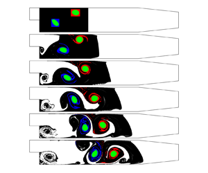
Figure 6 presents the PRA fields obtained at eight equal intervals throughout the flow cycle. Unlike FTLE, which characterizes the stretching factor of the deformation gradient matrix, PRA characterizes the rotational factor of the deformation gradient matrix. As a result, PRA readily locates Lagrangian coherent vortices, giving a fast computational approach before utilizing geodesic theory to detect elliptic LCSs. From figure 6 it can be seen that the main structures and evolution of the PRA fields are similar to those of the corresponding FTLE fields. However, the coherent vortices are more obvious in the PRA fields and the boundaries of vortex regions can be readily identified, something FTLE cannot do. The interior of a Lagrangian coherence vortex contains a series of concentric red and blue rings, indicating that the PRA value of fluid in a coherence vortex region changes continuously along its radial diameter. In areas of strong mixing, the colour of the PRA field is chaotic, suggesting that there is no specific law for the PRA of the fluid. Figure 6 illustrates the evolution of two Lagrangian coherent vortices, consistent with V1 and V2 considered in the previous section.

Figure 6. Polar rotation angle fields obtained over the period  $[t_0,t_0+T]$. Each plot is obtained by integrating trajectories of a uniform grid of
  $401\times 200$ particles using an integration interval of 0.020 s. Results are shown for (a)
  $t_0$, (b)
  $t_0+T/8$, (c)
  $t_0+2T/8$, (d)
  $t_0+3T/8$, (e)
  $t_0+4T/8$, ( f)
  $t_0+5T/8$, (g)
  $t_0+6T/8$ and (h)
  $t_0+7T/8$.
We utilize geodesic LCS theory to obtain the exact Lagrangian vortex boundaries. Figure 7 shows the hyperbolic LCSs and elliptic LCSs at the start of the cycle ( $t = 0.121\ \textrm {s}$) extracted using MATLAB packages developed by Onu, Huhn & Haller (Reference Onu, Huhn and Haller2015). The background comprises the FTLE field. The red and blue dots represent local
  $\lambda _2$ extreme points and local
  $\lambda _1$ extreme points, respectively. Repelling and attracting LCSs are given by shrink and stretch lines passing through these local extrema, and so are the most repelling and attracting material lines locally in the flow field. By considering the material lines, it can be seen that the repelling LCSs and FTLE ridges coincide closely, and hyperbolic repelling and attracting LCSs are perpendicular to each other. These two types of LCS partition the flow field into a net of local saddle regions, a concept borrowed from classical dynamical systems theory, leading to strong fluid mixing at the vortex periphery. A set of generalized saddle regions exists in the flow pathway observed in figure 5(a), suggesting that fluid elements close to these saddle points will be stretched and compressed significantly. The presence of repelling LCS in this region also supports the hypothesis that fluid particles starting on opposing sites of the repelling LCS will separate from each other.

Figure 7. Repelling LCSs (red), attracting LCSs (blue) and elliptic LCSs (green) near the BFS based on geodesic theory, with FTLE shown in the background.
In figure 7 the green dashed line indicates the Poincaré section used to determine isolated closed orbits (limit cycles) of the two explicit differential equations (2.14). The free stretching parameter  $\lambda$ in (2.15) is varied over the range
  $[0.90, 1.10]$ with increments of 0.02. Each green closed curve refers to the outermost elliptic LCS and corresponds to the Lagrangian vortex boundary, which exhibits no filaments during advection, and no leakage of fluid particles from within the orbits.
Now we compare the difference in vortex identification between Lagrangian and several Eulerian approaches. The simplest way is by using closed streamlines to locate vortices, as shown in figure 8(a). Areas with significant vortical patterns are identified. However, the presence of regions with many closed streamlines does not necessarily imply the existence of coherent vortices in an unsteady flow, such as the vortical structures near the left corner in the case considered here. These vortical structures cannot be guaranteed to preserve their shape during advection. Besides, the outermost closed streamlines are always larger than the actual coherent vortices (such as the region where V1 exists). Even worse, Lagrangian coherent vortex V2 is not completely contained in the closed streamline regions near the upper wall. The foregoing demonstrates that closed streamlines are weakly related to coherent vortices in an unsteady flow.

Figure 8. (a) Instantaneous streamlines, (b) instantaneous vorticity contours and (c) instantaneous zero level curves of  $Q$ at the start of the cycle (
 $t = 0.121\ \textrm {s}$) with two elliptic LCSs shown in green.
Consider the vorticity contours with Lagrangian vortex boundaries in figure 8(b). Although vorticity contours locate vortex boundaries more precisely than streamlines, discrepancies still occur. For instance, vorticity contours near the Lagrangian vortex boundary of V1 exhibit several filaments, which prevent its coherence being preserved under advection. On the other hand, there is no objective criterion for selecting an appropriate vorticity contour to approximate the boundary. Moreover, advection is also required to confirm the coherence of the chosen vorticity contour.
Finally, we use the  $Q$-criterion to detect vortical structures. The definition of
  $Q$ is
 \begin{equation} Q = \tfrac{1}{2}\left(\lVert \boldsymbol{\mathsf{A}} \rVert^{2}_F - \lVert \boldsymbol{\mathsf{S}} \rVert^{2}_F \right), \end{equation}
where
 $$\begin{gather} \boldsymbol{\mathsf{A}} = \tfrac{1}{2}\left(\boldsymbol{\nabla} \boldsymbol{u}-(\boldsymbol{\nabla} \boldsymbol{u})^{\mathrm{T}}\right), \end{gather}$$
 $$\begin{gather}\boldsymbol{\mathsf{S}} = \tfrac{1}{2}\left(\boldsymbol{\nabla} \boldsymbol{u}+(\boldsymbol{\nabla} \boldsymbol{u})^{\mathrm{T}}\right). \end{gather}$$
Vorticity dominates the region where  $Q>0$, whereas strain dominates the region where
  $Q<0$. Therefore, the zero contours are supposed to approximate vortex boundaries. However, the comparison in figure 8(c) indicates that zero contours of
  $Q$ will not necessarily delineate vortical structures, especially vortex V1. As for V2, the nearby closed contour is larger than the actual coherent vortex.
4.4. Evolution of Lagrangian coherent vortices
In figure 9(a) each green closed curve delineates the outermost member of the family of elliptic LCSs extracted according to geodesic theory (see § 4.3), and, hence, represents the boundary of a Lagrangian coherence vortex at the start of the cycle ( $t = 0.121$ s). In each elliptic LCS, the black ‘
 $\times$’ indicates the centre of the coherent vortex determined by local extreme points of the PRA. Red and blue dots indicate passive tracers within the vortex at different distances from the vortex centre (their
  $x$ ordinates are consistent with the vortex centre). The black curves describe trajectories of the vortex centres, and the red and blue curves indicate trajectories of the red and blue passive tracers. In figure 9(a) it can be seen that the trajectories of the red and blue dots invariably surround the vortex centre trajectory. Taking the vortex V2 as an example, figure 9(b,c) depicts the
  $x$- and
  $y$-coordinate time histories of the vortex centre and the two tracers. The red and blue tracers oscillate about the centre of the vortex, whereas the black tracer at the vortex centre experiences minimal oscillation. We also advect these two elliptic LCSs over the same time interval
  $[0.121\ \textrm {s},0.141\ \textrm {s}]$, as shown in figure 10. The advected curves appear to maintain good coherence during this time interval. Figures 9 and 10 therefore give a satisfactory representation of the coherence of the vortices in flow past a BFS.

Figure 9. (a) Trajectories of centres of Lagrangian coherent vortices (black  $\times$) and adjacent passive tracers (blue and red). (b,c) Time-dependent coordinates of vortex centres and adjacent tracers of vortex V2.

Figure 10. Evolution of elliptic LCSs over a time interval of 0.020 s. Elliptic LCSs are plotted at intervals of 0.002 s. The dashed line represents vortex V1 and the solid line represents vortex V2.
Figure 11 verifies this property of elliptic LCSs. The first panel shows the distribution of fluid particles at the start of the cycle. The green area depicts fluid particles inside the elliptic LCSs. Red and blue areas are used to assist in visualizing the movement of fluid particles around the elliptic LCSs. The six panels display results at intervals of 0.004 s, starting at 0.121 s and ending at 0.141 s. From figure 11 it can be seen that even when fluid particles in the red and blue areas are dispersed and filaments appear, fluid particles do not leak out from the vortex, which maintains its coherence throughout the time considered. By comparison with the coherent vortex in figure 6, it is found that at the same moment, the shape, size and position of both vortex structures are very consistent. Therefore, even for different finite-time dynamic systems, the detected structures can indeed evolve each other.

Figure 11. Distribution of fluid particles whose initial positions are inside (green) and outside (red and blue) the elliptic LCSs over a time interval of 0.020 s.
Next, we investigate the vorticity fluxes of the Lagrangian coherent vortices V1 and V2. In order to evaluate the vorticity fluxes of the Lagrangian vortices over time, it is necessary to materially advect the elliptic LCSs under the flow map and to integrate vorticity inside the elliptic LCSs at different time instants. The evolution of elliptic LCSs represents the evolution of boundaries of Lagrangian vortices, as shown in figure 10. Figure 12 shows the resulting flux time histories. At the initial time, the vorticity fluxes of the two coherent vortices are almost the same, except that one is positive and the other is negative. The upper coherent vortex V2 has a flux of  $3.1217\times 10^{-4}\ \textrm {m}^{2}\ \textrm {s}^{-1}$ whereas that of the lower coherent vortex V1 is
  $-3.1837\times 10^{-4}\ \textrm {m}^{2}\ \textrm {s}^{-1}$. This indicates that their rotation directions are opposite and their strength is similar. The vorticity fluxes decrease slightly with time. This decrease may be caused by fluid viscosity, numerical dissipation, etc., and requires further research. At the end time, the flux of vortex V2 is
  $2.9282\times 10^{-4}\ \textrm {m}^{2}\ \textrm {s}^{-1}$ and that of vortex V1 is
  $-2.9931\times 10^{-4}\ \textrm {m}^{2}\ \textrm {s}^{-1}$, which are 93.8 % and 94.0 % of the initial flux, respectively. As illustrated in figure 12, the strength of these two coherent vortices remains almost constant throughout the time considered, with their sum flux invariably remaining close to zero, revealing that the vortex generated by boundary layer separation at the upper wall and the vortex generated by the separated shear layer bounding the recirculation region are both self-sustaining and have very similar strength.

Figure 12. Time histories of the individual and summed vorticity fluxes of the two Lagrangian coherent vortices, V1 and V2.
5. Conclusions
Finite-time Lyapunov exponent, PRA and geodesic LCS methods have been used to determine Lagrangian coherent structures in flow past a BFS at Reynolds number  $Re = 5080$. Although these methods have been widely used in the realm of unbounded geophysical flows, this paper presents the first application of a combination of such methods to flow past a BFS, demonstrating the potential role of LCS in the analysis of coherent structures in bounded flows.
In Lagrangian analysis, choice of a proper integration interval is important. From our perspective, the general procedure should comprise the following steps. First, devise a proper set of integration intervals, based on the time scale of the specific flow and the amount of available velocity data in both space and time. Next, advect seed points in the flow region of interest for different time intervals over the set of integration intervals (which can be undertaken in a single numerical integration routine). Finally, compare the visual results and adopt the integration interval whose visualization extracts the most important LCSs at relatively low computational cost.
Our results have shown that the underlying structures within the BFS flow are properly detected by combination of qualitative and quantitative LCS analysis methods. The FTLE and PRA diagnostic methods have a well-defined duality in that they respectively characterize the stretching and rotation of an infinitesimal fluid sphere. The FTLE value is extremely small at the core of a vortex, and very large at its periphery. Correspondingly, the PRA value remains regular in coherent vortical regions but becomes random in chaotic mixing zones. From our simulations, we find that a flow pathway in which fluid particles hardly diverge from their immediate neighbours is opened and closed periodically by FTLE ridges associated with the shedding of vortices. The pair of dominant Lagrangian coherent vortices is visualized more clearly by PRA. A quantitative study of geodesic LCSs reveals that the two dominant vortices are described by elliptic LCSs with no filaments present during advection and no leakage of interior fluid particles. Moreover, the strength of these two coherent vortices is nearly constant with time and the sum of their fluxes remains close to zero, indicating that the vortices are self-sustaining and of similar strength. Hyperbolic repelling and attracting LCSs that are orthogonal to each other partition the flow field into a net of local saddle regions, a concept borrowed from classical dynamical systems theory, which results in intensified fluid mixing. These most repelling, attracting and shearing material lines serve as key elements of complicated tracer patterns in BFS flow.
The fluid mechanics behind the spatiotemporal formation and development of coherent vortices in BFS flow is still not fully understood. Interactions between the different geometric regions partitioned by LCSs lead to the intrinsic complexity of BFS flow. It is recommended that future research examines the effect of modifying the shape of the BFS on coherent structures and mass and energy transfer through the flow pathway (of importance to combustion). Attention should also be paid to more effective flow control methods. Although self-sustaining vortex formation is widely acknowledged as an important component of separated flow, the development of a universal flow control approach remains a scientific and technological challenge, with little agreement achieved to date between results from previous experimental and computational studies. It is therefore useful to investigate the coherent structures and dynamic characteristics of BFS flow over a broad range of Reynolds numbers, which could lead to discovery of an effective solution to the flow separation control problem for a duct containing a BFS.
Acknowledgements
The first author would like to thank Dr B. Xie from SJTU for sharing the high-fidelity CFD code. The authors are also grateful to the anonymous referees for their helpful comments and suggestions.
Funding
The authors acknowledge support from the National Natural Science Foundation of China (grant no. 51979162 and no. 52088102).
Declaration of interests
The authors report no conflict of interest.


