


1. Introduction
Recirculating flow is ubiquitous, whether beneficial (e.g. enhanced mixing) or detrimental (e.g. increased drag) to overall function. Recirculation is characterized by a region of separation that features retrograde flow, increased mixing and trapped fluid parcels. In a combustor, fuel-rich cold air must effectively mix with hot combustion products (Gruber et al. Reference Gruber, Donbar, Carter and Hsu2004; Cai et al. Reference Cai, Sun, Wang and Bai2018). Also, efficient mixing and control of residence times is crucial in flow reactors (Gobert et al. Reference Gobert, Kuhn, Braeken and Thomassen2017; Reis, Varner & Leibfarth Reference Reis, Varner and Leibfarth2019). In a biological context, however, recirculating blood flow behind a stenosis or in an artificial heart can lead to complications if allowed to stagnate (Martorell et al. Reference Martorell, Santomá, Kolandaivelu, Kolachalama, Melgar-Lesmes, Molins, Garcia, Edelman and Balcells2014; Sonntag et al. Reference Sonntag, Kaufmann, Büsen, Laumen, Gräf, Linde and Steinseifer2014). Thus, effective mixing and fluid exchange across the shear layer, between the free stream and a recirculation region, play a key role in a myriad of industrial and biological applications alike.
1.1. Depletion of a recirculating fluid
Figure 1 depicts mixing between a steady or unsteady jet and an adjacent recirculation region, where entrainment across the shear layer allows recirculating fluid to be flushed from the domain. In the current study, this action, and its associated rate, are referred to as ‘depletion’ and ‘depletion efficiency’, respectively. To date, few studies within the fluids community have evaluated recirculation depletion mechanics and their efficiency. A study by Noack et al. (Reference Noack, Mezić, Tadmor and Banaszuk2004) on optimal mixing analysis in recirculation zones demonstrated that one could increase depletion of fluid from a recirculation zone by modifying vortex motion to maximize flux and decrease particle residence time (PRT). Piccolo, Arina & Cancelli (Reference Piccolo, Arina and Cancelli2001) identified an increase in the transport rate of fluid behind a backward-facing step as a function of the Strouhal number of the external flow. Sonntag et al. (Reference Sonntag, Kaufmann, Büsen, Laumen, Gräf, Linde and Steinseifer2014) applied a similar concept to the ‘washout’ efficiency of an artificial heart using pulsatile flow and measured the volume of fluid depleted for different inlet configurations. However, to the authors’ knowledge, no study exists comparing the depletion efficiency for steady and pulsatile flows. Furthermore, the physical mechanisms responsible for these mixing processes are poorly understood.

Figure 1. Flow through an axisymmetric stenosis geometry causes the depletion of fluid recirculating downstream of the obstruction. Black and red lines represent fluid exiting the axisymmetric stenosis throat, while the blue and green lines denote fluid that is depleted from the region by the inflow or that enters from downstream, respectively. (a) Steady flow can be associated with Kelvin–Helmholtz (KH) instabilities along the shear layer (dotted red area), while (b) pulsatile flow forms a vortex ring at every pulse (dotted blue area). In the current study, the focus is on the behaviour of the recirculating fluid (blue arrows) in response to the jet fluid (red arrows).
1.2. Steady versus pulsatile flows
In this study, an idealized stenosis geometry is used to generate a large recirculation region within which the depletion efficiency of pulsatile flows is investigated, in pure liquid, dilute and dense suspensions. For a pulsatile inlet condition, the growth, propagation and shedding of a coherent vortex ring, as illustrated in figure 1(b), has been documented in the post-stenotic region during the acceleration and deceleration phases of each pulse (Blackburn & Sherwin Reference Blackburn and Sherwin2007; Varghese, Frankel & Fischer Reference Varghese, Frankel and Fischer2007b; Blackburn, Sherwin & Barkley Reference Blackburn, Sherwin and Barkley2008). Additionally, studies by Stewart et al. (Reference Stewart, Niebel, Jung and Vlachos2012) and Zhang & Rival (Reference Zhang and Rival2020) both discuss the generation of vortex rings by a confined, pulsed jet (using a piston pump) for Reynolds numbers up to 12 000. When the flow is steady, however, no vortex rings are formed and mixing is limited to Kelvin–Helmholtz (KH) instabilities, along the shear layer, which form small vortical structures that quickly decay in high-Reynolds-number flows (Varghese, Frankel & Fischer Reference Varghese, Frankel and Fischer2007a; Cantwell, Barkley & Blackburn Reference Cantwell, Barkley and Blackburn2010). It is these coherent structures that are a significant contributor to entrainment within the recirculation region and may accelerate depletion (Shadden, Dabiri & Marsden Reference Shadden, Dabiri and Marsden2006). In a similar fashion, Ruiz, Whittlesey & Dabiri (Reference Ruiz, Whittlesey and Dabiri2010) explored the viability of vortex-enhanced propulsion by means of a pulsed jet. They demonstrate that the generation of coherent vortical structures in an unsteady jet can improve propulsive efficiency when compared to an equivalent steady jet. In fact, Ruiz et al. (Reference Ruiz, Whittlesey and Dabiri2010) identify conditions whereby the added power consumption of the unsteady flow is offset by the performance increase. This result begs the following question: Can pulsatile internal flow featuring the rollup of large-scale vortex rings improve mixing and the overall depletion efficiency?
1.3. Mixing in suspensions
Extending this question of pulsatile depletion efficiency to dilute and dense suspensions is not straightforward, and vortex-dominated mixing dynamics, unlike in pure-liquid flows, are not well understood. Characterizing the behaviour of these suspensions is heavily predicated on the interaction between the suspended phase and the liquid carrier. Furthermore, and until recently, it has been difficult to investigate suspensions experimentally – particularly those of significant solid/liquid volume fractions – due to their opacity, which hinders traditional optical measurement techniques. The current study extends its analysis of depletion efficiency to dilute and dense suspensions by using a refractive index matching technique (Wiederseiner et al. Reference Wiederseiner, Andreini, Epely-Chauvin and Ancey2010). Recently, studies using super-absorbent hydrogel beads of various diameters have demonstrated turbulence attenuation and vortex formation dynamics in dense suspensions with volume fractions up to 25 % (Zhang & Rival Reference Zhang and Rival2018; Baker & Coletti Reference Baker and Coletti2019; Zhang, Jeronimo & Rival Reference Zhang, Jeronimo and Rival2019; Zhang & Rival Reference Zhang and Rival2020). However, much is still unknown about the contribution of the suspended phase in the entrainment process of pulsatile recirculating flows.
1.4. Measuring depletion efficiency
The objective of the current study is to characterize how efficiently steady and pulsatile flows can deplete a recirculating region of stagnant fluid. Section 2 describes the use of Lagrangian measurement techniques to track fluid parcels exiting a stenosis and their interaction with the recirculation region. The interactions occurring across the shear layer are observed in § 3.1 and are investigated for increasing Reynolds number and varying degrees of pulsatility (unsteadiness). In § 3.2 key depletion mechanisms are quantified and discussed with the aim of assessing the depletion efficiency for steady and pulsatile flows. Furthermore, in § 3.3, the Lagrangian analysis of recirculating fluid is extended to dilute and dense suspensions in order to investigate how the presence of suspended particles alters fluid entrainment across the shear layer.
2. Methods
2.1. Experimental facility
The depletion efficiency of steady and pulsatile flows was evaluated using the flow loop and idealized stenosis model shown in figure 2. The working fluid – either pure water or a suspension of aqueous hydrogel beads in deionized water (described in detail in § 2.2) – was pumped from the reservoir and around the flow loop using a programmable circumferential piston pump (Wrightflow TRA10 Model 1300). The pump is designed to function for pure liquid or dense slurries and provides low shear, which ensures damage to the hydrogel beads is minimal. The flow rate of the pump is controlled by sending an analogue signal to the pump controller (using LabView) that describes the desired steady or pulsatile profile.

Figure 2. (a) A render of the optical test section and fluid reservoir parts of the experimental facility. A pump (not shown),  $60D$ upstream of the optical test section, generates flow from left to right through the stenosis model (circled), which is immediately followed by the region of interest used for 2-D PTV. (b) A close-up view of the test section with a
  $90^{\circ }$ cutaway of the stenosis model showing its curvature.
Two-dimensional particle tracking velocimetry (2-D PTV) was performed in the test section, a 1 m long acrylic pipe with an internal diameter of  $D=7.6$ cm housing the stenosis model, as illustrated in figure 2(a). The onset of the pipe's constriction (stenosis) was situated approximately 60 diameters downstream of the nearest corner to ensure that turbulent flow conditions could be considered fully developed. The constriction was adapted from generic stenosis models typically found in the literature (Blackburn & Sherwin Reference Blackburn and Sherwin2007) and consists of a contraction of the inner pipe diameter by 50 % (the throat area is 25 % of the pipe's cross-sectional area) immediately followed by a sudden expansion back to
  $D$ (see figure 3).

Figure 3. A cross-sectional slice, along the centre plane of the light sheet of the stenosis model, as used in this study. The axisymmetric stenosis reduced the diameter of the pipe by 50 %, and the cross-sectional area by 75 %, before rapidly expanding to create a jet and a large recirculation region. The region of interest covers half of the pipe diameter and is highlighted using a white box. Within this domain, scattered Lagrangian vector data (blue arrows) were processed into long pathlines (orange and black lines). The origin  $(0,0)$ of the measurement domain is at the edge of the stenosis (red dot).
The axisymmetric contraction is described by the smooth sinusoidal curve  $r(x)$ for
  $-0.5 \leqslant x/L < 0$, as follows:
 \begin{equation} r(x)=\frac{1}{2}\left[d+(D-d)\sin^2\left(\frac{{\rm \pi} x}{2L}\right)\right], \end{equation}
where  $x$ is the position along the pipe,
  $d = D/2$ is the stenosis throat diameter and
  $L = 7.6$ cm is the length of the stenosis. This canonical geometry generates a large region of recirculating fluid that was crucial to studying the effects of pulsatility on the depletion efficiency of pure-liquid flow, as well as dilute and dense suspension flows.
The acrylic test section (containing the stenosis model) was encased in an octagonal tank, which, when filled with water, rendered the curved walls of the pipe optically transparent and reduced the effect of any aberrations. A high-speed complementary metal oxide semiconductor (CMOS) camera (FASTCAM Mini WX100), with an  $f=60$ mm Nikon lens and set at a resolution of
  $2048 \times 1120$ pixels (0.03 mm pixel
 $^{-1}$), recorded flow exiting the throat of the stenosis. The camera was positioned to capture a field of view 6.1 cm by 3.8 cm (
 $1.6d \times 1.0d$), extending downstream from the edge of the stenosis and radially from the wall to the pipe centreline (as shown in figure 3). When extending pathlines and calculating path-dependent quantities in the following sections, the measurement domain is identical to the camera's field of view. The frame rate (up to 2000 Hz) was changed according to the peak Reynolds number to ensure that inter-frame particle displacements did not exceed a maximum of 15 pixels. The camera's exposure time was set from 1/4000 s to 1/8000 s, depending on the peak flow velocity, so that particle images did not appear as streaks. A 3 W diode-pumped continuous solid-state laser (532 nm) was used to produce a laser sheet along the axis of the pipe such that 2-D PTV could be performed in the region immediately following the sudden expansion. For pulsatile flow cases, the camera and mean flow profile were synchronized using a digital acquisition device (National Instruments USB-6351) so as to always begin recording at the same instant of each pulse (
 $t/T=0$).
2.2. Hydrogel beads – making a dense suspension
Recirculation region dynamics were studied for both pure water and suspensions. The suspensions were mixed using deionized water and hydrogel beads made of a super-absorbent polymer (SAP), purchased from Emerging Technologies (LiquiBlock 2G-110), that are uniformly dispersed in water (from this point forward we refer to the suspended phase as ‘hydrogel beads’ or simply ‘beads’). The hydrogel beads have a water absorption coefficient of 450 g of water per gram of the polymer. When fully saturated in water, the beads’ refractive index matches that of water and the resulting suspensions are optically transparent (Wiederseiner et al. Reference Wiederseiner, Andreini, Epely-Chauvin and Ancey2010). Furthermore, the high absorbency of the polymer means that the mass and hence the density of the solid–liquid mixture is practically identical to that of pure water. When saturated, the bead diameter ranges from  $d_p=0.8$ to 1.4 mm (0.01
 $D$ to 0.02
  $D$), and the mean bead aspect ratio is approximately one.
For the current study, the working fluid was characterized by the volume fraction,  $\varPhi$, of solid hydrogel beads to deionized water. Dilute (
 $\varPhi =5\,\%$) and dense (
 $\varPhi =10\text {--}20\,\%$) suspensions, as well as pure-liquid flows (
 $\varPhi =0$) were each evaluated. A dense suspension is classically defined as one where the separation between disperse particles is of the same order as or smaller than the diameter of the solid particles (Stickel & Powell Reference Stickel and Powell2005). The mean inter-particle spacing, normalized by the bead diameter, is
  $l_p/d_p \approx 2.3$, 1.9 and 1.5 for the
  $\varPhi =5\,\%$, 10 % and 20 % suspensions, respectively, where
  $l_p$ is the centre-to-centre distance between hydrogel beads and
  $l_p/d_p \leq 2$ for dense suspensions (Kryuchkov Reference Kryuchkov2001). The settling velocity of the hydrogel beads has previously been measured at approximately
  $0.6\pm 0.3$ mm s
 $^{-1}$ (Zhang & Rival Reference Zhang and Rival2018) and is very low when compared to the convective speeds of the system. Furthermore, the concentration of beads in the current tested suspensions is sufficiently high that these particles cannot be considered to move (settle) in isolation of one another. Balachandar & Eaton (Reference Balachandar and Eaton2010) provide a detailed review of the coupling between dispersed and carrier phases for dilute suspensions, as well as the effect of volume fraction on the modulation of carrier-phase turbulence.
Large volumes of each suspension were prepared in batches by first degassing the deionized water, then thoroughly mixing in the hydrogel beads, and then finally degassing again. The suspension was added to the flow-loop reservoir and allowed to pump through the test section for approximately one hour before testing to ensure the hydrogel was uniformly distributed throughout the post-stenotic region. As  $\varPhi$ is increased, the number of hydrogel–water interfaces between the camera and the imaging plane increases. At each interface there is a slight refractive index mismatch that begins to significantly degrade image quality above
  $\varPhi =20$ %, where imaging occurs through approximately 40 interfaces.
2.3. Steady and pulsatile flow parameters
The depletion of recirculating fluid from the post-stenotic region was investigated for increasing mean Reynolds number ( $Re$), Strouhal number (
 $St$) and amplitude ratio (
 $\lambda$), as well as the four volume fractions (
 $\varPhi$) previous outlined. Table 1 shows the range of values of each parameter. The Reynolds number
  $Re_m= u_m d/\nu$ of the working fluid was calculated using the mean flow velocity (
 $u_m$), the diameter of the stenosis throat (
 $d$) and the kinematic viscosity (
 $\nu$) of the liquid phase. All relevant convective scales were normalized by the throat of the contraction where the characteristic length is
  $d= 3.8$ cm. The pulsatile test cases are periodic and can be described as the sum of a sinusoid – with frequency
  $f_p$ and amplitude
  $u_o$ – and a steady flow with a mean velocity
  $u_m$, as depicted in figure 4.

Figure 4. The pulsatile flows investigated are characterized by an amplitude ratio,  $\lambda =u_o/u_m$, and a Strouhal number,
  $St=f_p d/u_m$, where
  $d$ is the stenosis throat diameter and
  $f_p$ is the frequency. This schematic shows the relative size of the three amplitude ratios (solid lines) and the frequency of the three Strouhal numbers (dashed lines).
Table 1. Parameter space and range used in the current study.

The steady and pulsatile waveforms were verified using particle image velocimetry (PIV) measurements of the jet within a small domain, with dimensions  $0.8d \times 0.8d$, and centred along the pipe's axis. Figure 5 shows the jet velocity waveform measured using PIV for a pulsatile flow with
  $Re=9600$,
  $St=0.08$ and
  $\lambda =0.50$. The mean velocity, amplitude and frequency were measured within
  $\pm 5\,\%$,
  $\pm 10\,\%$ and
  $\pm 2\,\%$ of the expected values, respectively, and a small phase lag was accounted for when analysing the recirculating flow. In dimensionless form, pulsatile flow is characterized by a Strouhal number
  $St=f_p d/u_m$ and an amplitude ratio
  $\lambda =u_o/u_m$. The period (
 $T$) ranges from 0.66 s to 8 s at the extremes of
  $St$ and
  $u_m$.

Figure 5. The mean jet velocity measured using PIV is shown compared to the input waveform to the circumferential piston pump. In this exemplary case, the fluid waveform closely follows the input at  $Re=9600$,
  $St=0.08$ and
  $\lambda =0.50$ in a pure liquid (
 $\varPhi =0$%).
Pulsatile flows are often characterized by a Womersley number, which is another frequency-dependent parameter that describes the significance of inertial effects in the presence of an oscillating pressure gradient. However, the Womersley number can be seen as simply the product of the Strouhal and Reynolds numbers, and the same value can represent vastly different flow conditions. While discussing its use in biological flows, Rohlf & Tenti (Reference Rohlf and Tenti2001) recommended that the Womersley number should be used as an indicator of when non-Newtonian effects are important, and not for characterizing pulsatile flows. The upper limit on  $\lambda$ was set below one to avoid flow reversal upstream (oscillatory flow) and to prevent the pump reaching a flow rate of zero.
Comparing the behaviour of pure-liquid flow with that of a suspension can be very challenging. Suspensions cannot be assumed to act as a continuum and the application of an effective viscosity and matching Reynolds number is not sufficient (Guazzelli & Pouliquen Reference Guazzelli and Pouliquen2018; Zhang & Rival Reference Zhang and Rival2020). In the current study, results are compared for matching mean velocity ( $u_m$) through the stenosis at each volume fraction, but, for simplicity, are referred to according to their equivalent pure-liquid Reynolds number (ranging from 4800 to 14 400).
2.4. Two-dimensional particle tracking
Lagrangian particle tracking of the liquid phase was performed in the region downstream of the stenosis model by seeding the working fluid with neutrally buoyant 55  $\mathrm {\mu }$m polyamide tracer particles (LaVision 1108947). From this point onwards, the term ‘particle’ refers to the tracer particles that are seeded in the liquid phase. The tracer particles have a Stokes number of the order of
  $10^{-4}$ and are assumed to reliably follow the motion of the liquid. Note that, while the motion of the particles is affected by the presence of the hydrogel beads, the solid phase itself is not directly tracked. Particle detection and matching are negatively affected by high particle image density, as particle identification becomes ambiguous. Here, the particle image density is approximately 0.0015 particles per pixel (ppp) and 3000 particles are detected in each frame. Given the turbulent nature of the flows under investigation, there is likely to be particle loss due to out-of-plane motion with a thin light sheet. Rosi, Walker & Rival (Reference Rosi, Walker and Rival2015) discuss out-of-plane motion as an indirect source of error in 2-D tracking measurements that is inversely proportional to the laser sheet thickness so long as the reduction of the sheet's energy density does not jeopardize particle image density.
To ensure tracers can be tracked across as many frames as possible, the laser sheet was set to a thickness of approximately 5 mm. The camera lens was set to  $f_\#=16$ such that the depth of focus can be estimated at 4.4 mm (Raffel et al. Reference Raffel, Willert, Scarano, Käehler, Wereley and Kompenhans2018), ensuring the particle images remained in focus across the entire depth of the light sheet. For 2-D tracking measurements, where particle density (and overlap) is relatively low, a thick light sheet compensates for out-of-plane motion and yields longer particle tracks (Cierpka, Lütke & Kähler Reference Cierpka, Lütke and Kähler2013). Although, the thick sheet may introduce some spatial averaging across the depth of the laser sheet (of the order of 0.06
 $D$), ultimately we are tracking individual tracer particles such that this averaging will not negatively affect the (Lagrangian) pathline extension process (as described below).
The 2-D PTV was performed using LaVision DaVis 8.4.0 software. Images were first filtered using a mean background subtraction across all frames, as well as a second mean subtraction over only 15 frames to remove small reflection artifacts from the pipe wall. Particle detection used a Gaussian fit followed by peak intensity detection to find particles in each frame. Velocity vectors were then drawn for each particle's displacement by connecting them from frame to frame using peak matching within an allowable velocity range (Dracos Reference Dracos1996). The spatial coherence of each displacement vector is compared to neighbours within a 50-pixel radius before verifying the displacement as valid and drawing a track between the corresponding frames.
The uncertainty in detecting a particle's position using PTV depends on particle overlap and ambiguity and hence increases at high particle image density. The density is carefully controlled to avoid particle ambiguity and, with a particle image diameter of approximately four pixels, the positional uncertainty is of the order of 0.1 pixels for a 2-D Gaussian fit (Kähler, Scharnowski & Cierpka Reference Kähler, Scharnowski and Cierpka2012). Full particle tracks are filtered once more to eliminate very short tracks that would otherwise contribute to noise. A valid track must extend across at least five consecutive frames and no single step may differ by more than 20 % of the previous step; i.e. a sudden acceleration from one displacement to the next would be non-physical. Increasing the acceptable track length lowered the number of valid tracks, while decreasing the threshold had no significant effect on track density. Ultimately, low track density and very short tracks both had a negative effect on pathline extension and influenced the chosen threshold. The following section describes how approximately 2000 valid particle tracks in each frame are extended to reveal their history.
2.5. Pathline extension
The source and terminal positions of each tracer particle that was tracked moving through the measurement domain were computed by extending pathlines to reveal their individual trajectories. Pathline extension, as described by Jeronimo, Zhang & Rival (Reference Jeronimo, Zhang and Rival2019) and Jeronimo & Rival (Reference Jeronimo and Rival2020), uses a set of flow maps fitted to the displacements measured for each time step to predict the motion of particles throughout the measurement domain (as defined by the camera's field of view). This extension method was inspired by flow-map compilation techniques (Brunton & Rowley Reference Brunton and Rowley2010; Raben, Ross & Vlachos Reference Raben, Ross and Vlachos2014; Rosi & Rival Reference Rosi and Rival2018). Flow maps are a surface fit of the displacements of particles between consecutive frames and were computed for both forward and backward time steps using a locally weighted scatter-plot smoothing algorithm (LOWESS). The end points of each measured track were then extended by interpolating from the time-resolved flow maps.
The uncertainty associated with extending pathlines can be estimated by comparing the measured frame-to-frame displacements of particles (in Cartesian space) at a given time step to the displacements calculated by the flow map for that same time step. Computing the magnitude of the residuals between measurements and the flow map predictions yields a normalized mean error of  $\pm$5 %, which was consistent across all flow maps. The mean error is a measure of how accurately the flow maps fit the physical data points that represent the position and motion of particles tracked at each time step. Residuals are calculated individually for each flow map (one for each of the up to 6000 time steps) such that the 5 % error is consistent regardless of the extended path length or final position of the fluid parcel, and does not grow exponentially for long pathlines. The resulting pathlines describe the lifespan of each unique fluid parcel within the measurement domain and can be used to extract path-dependent quantities, including PRT and velocity. The extended pathlines have an average length of approximately 1000 time steps – some 50 times their original length. A detailed description of the pathline extension methodology can be found in Jeronimo et al. (Reference Jeronimo, Zhang and Rival2019) and Jeronimo & Rival (Reference Jeronimo and Rival2020).
3. Results and discussion
Pathline extension reveals the trajectories of every unique particle that is detected in the measurement domain along which path-dependent dynamics can be extracted. Section 3.1 highlights the methods of categorizing and quantifying scattered Lagrangian data that are most useful for tracking depletion and vortex dynamics in the recirculation region. The mechanisms that are identified therein are investigated in §§ 3.2 and 3.3 to reveal the effects of pulsatility and suspension density on depletion efficiency, in both pure-liquid and suspension flows.
3.1. Extracting path-dependent dynamics
3.1.1. Trajectory-based labelling
Lagrangian pathline extension allows the time-resolved positional information describing the transit of individual flow tracers through the measurement domain to be extracted from scattered 2-D PTV data. Using this information, the tracked liquid-phase fluid parcels can be labelled by any number of means, e.g. by source coordinates or time spent in a specific region. To highlight the depletion of recirculating fluid, fluid parcels are categorized by their initial position and their interaction with the shear layer that extends out from the edge of the stenosis throat.
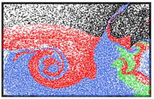
Figure 6 shows scattered particles coloured according to the flow depiction in figure 1. The four flow categories are defined as follows: fluid initially in the recirculation region (any particle below  $y/d=0$ at
  $t/T=0$) is blue (Recirculating); jet fluid is coloured red if it crosses the line
  $y/d=0$ into the recirculation region (Entrained) and is otherwise black (Jet); and green particles represent fluid entering the domain after
  $t/T=0$ and from the right-hand side of the frame (Downstream). The line
  $y/d=0$ is simply used as a threshold at
  $t/T=0$ to identify fluid that will be tracked as it is depleted from the measurement domain. The horizontal line
  $y/d=0$ coincides with the edge of the stenosis throat from which a shear layer extends across the length of the measurement domain. Other forms of division, such as a line describing the shear layer or the turbulent/non-turbulent interface, could be used but these are not easily defined or are equally arbitrary for the analysis performed herein. Note that the top row of figure 6 actually depicts a moment very shortly after
  $t/T=0$ such that the vortical structures already forming at
  $t/T=0$ can be observed.

Figure 6. Fluid parcels in the measurement domain are categorized according to their source position and trajectory thereafter. The volume of recirculating fluid is depleted by the motion of entrained jet fluid in the case of steady (left column) and pulsatile (right column) inlet flow. Vortex formation and shedding apparent during the acceleration phase ( $t/T=0\text {--}0.250$) for pulsatile flow is absent in the steady flow. KH instabilities and the gradual influx of downstream (green) fluid are seen throughout for the steady flow case. Both flows are compared at
  $Re=4800$ over the same length of time, which is normalized by the period (
 $T$) of the pulsatile flow (
 $\lambda =0.50$ and
  $St=0.08$). This steady and pulsatile flow comparison is animated in supplementary movie 1.
The side-by-side comparison of fluid motion within the recirculation region when subjected to steady and pulsatile inlet flows (in figure 6) highlights the key difference between their depletion mechanisms. For steady flow, the turbulent jet is separated from the recirculation region by a shear layer, wherein KH instabilities result that entrain small volumes of recirculating fluid; such small vortical structures are observed continually, as plotted in figure 6 over a period of  $T=4$ s. Retrograde flow from downstream is observed to consistently enter the region, and contributes to displacing recirculating fluid. The pulsatile flow is characterized by the formation of a vortex that is growing from
  $t/T=0$ to
  $0.125$. As the acceleration comes to an end (
 $t/T=0.250$), and the flow begins to slow, the vortex structure sheds and advects downstream, carrying fluid entrained from the recirculation region with it (see the blue fluid parcels rolled into the red jet fluid).
These vortex forming and shedding processes are periodic and can be seen to begin again as the flow accelerates up from its minimum velocity. In between the vortices, and during the deceleration of the pulsatile waveform, fluid from downstream flows into the domain and displaces recirculating fluid towards the centre of the pipe, where it can be forced out of the measurement domain. A large portion of the downstream particles (green) are then washed out again when the flow rate increases. In the select pulsatile cases where  $\lambda =0.95$, and the jet velocity briefly approaches zero, the amount of retrograde flow increases significantly, fluid is no longer trapped by the presence of a strong jet, and a large number of fluid parcels exit the recirculation region. By comparison, the lack of large velocity gradients in the steady case allows downstream fluid to more consistently, albeit slowly, enter the domain – green particles gradually flow into the domain from
  $t/T=0$ to
  $0.250$ in figure 6.
The post-stenotic vortex dynamics – for both the steady and pulsatile flows – can be seen in supplementary movie 1 (available at https://doi.org/10.1017/jfm.2021.752) for the flow conditions described in figure 6. Note that, while the particle image density was uniform during particle tracking, the distribution of particles after the pathline extension process is uneven, as seen in figure 6. This effect is caused by the large velocity difference between the jet, where the (post-extension) particle density is more sparse, and the recirculation region. Particles whose trajectories extended backwards into the jet are typically carried out of the domain quickly, while low-energy particles accumulate in the recirculation region and increase the local particle density. However, the analysis that follows in § 3.2 focuses on the initial group of particles in the recirculation region at  $t/T=0$ where the particle distribution is relatively uniform. The depletion mechanisms, and the influence of mean and pulsatile flow parameters, are discussed in more detail in the following sections.
3.1.2. Particle residence time
The scattered Lagrangian data can also be described by their PRT within the domain, as described by Jeronimo et al. (Reference Jeronimo, Zhang and Rival2019) and Jeronimo & Rival (Reference Jeronimo and Rival2020). Reza & Arzani (Reference Reza and Arzani2019) provide a detailed comparison of a variety of methods describing and calculating residence time. In this study, PRT is defined as the length of time a fluid parcel spends in a region of interest (Shadden & Arzani Reference Shadden and Arzani2015), and that can be directly computed by extending its pathline. Here, the region of interest is the entire field of view of the camera and PRT is tracked for each fluid parcel anywhere within this domain ( $0< x/d<1.6$ and
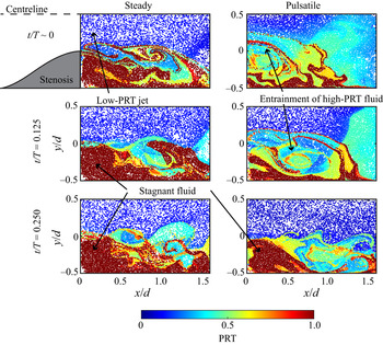
  $-0.5< y/d<0.5$). Figure 7 shows the acceleration phase of a pulsatile flow (and an equivalent duration of steady flow) labelled by the normalized PRT of particles, and identifies regions of high and low PRT. Low-PRT jet fluid is easily distinguished from fluid that mixes into the recirculation region, causing its PRT to grow. For both flows, there is a large concentration of high-PRT fluid near the walls of the pipe and stenosis that is not easily displaced. Jeronimo & Rival (Reference Jeronimo and Rival2020) reported an increase in the PRT of entrained jet fluid with the introduction, and strength, of pulsatility, and its direct correlation to large vortex structures.

Figure 7. The PRT of fluid in the recirculation region is compared for steady (left column) and pulsatile flow (right column) at  $Re=4800$,
  $\lambda =0.50$ and
  $St=0.08$. Concentrations of stagnant fluid, as well as the source of new high-PRT fluid, are easily identified. The mean PRT is higher in the steady flow case, while the vortex formed by the pulsatile flow exchanges new jet fluid for high-PRT fluid trapped in the recirculation region.
In the current study, the focus is to evaluate how efficiently stagnant, high-PRT fluid can be depleted from the recirculation region. Key differences in the PRT of fluid parcels subjected to steady and pulsatile flows are identified in figure 7. At each instant, the steady jet is predominantly low-PRT fluid, suggesting that the KH instabilities do not entrain jet fluid deep into the recirculation region, which, in turn, would promote depletion. As a result, there is a large volume of high-PRT fluid in the steady flow case. By comparison, the average PRT of jet fluid is greater for the pulsatile flow due to vortex formation that entrains new, high-PRT fluid down into the recirculation region. Over the course of the acceleration, the large vortex pushes high-PRT fluid out of the domain, resulting in a smaller amount of stagnant fluid compared to the steady case. The entrainment of high-PRT fluid during the growth and shedding of a coherent structure in the pulsatile flow suggests a higher depletion efficiency; more in-depth analysis of depletion efficiency for steady and pulsatile flows continues in § 3.2.
3.1.3. Vorticity
Using the time-resolved, scattered positional data available for each pathline, the velocity along the trajectories can be computed using a central difference method and the known frame-to-frame time step. The coherent vortical structures observed in figure 6 can be quantified by calculating the out-of-plane vorticity ( $\omega _z^*$) of the affected fluid parcels. To calculate vorticity, the Lagrangian velocity data are first interpolated onto a rectilinear grid, with a resolution of
  $0.005d$, and then differentiated. Spatial gradients were performed using a central differencing approach. The vorticity was then normalized using a convective time (
 $d/u_m$) and interpolated back on to the scattered data such that each pathline contains the vorticity history of the fluid parcel.
Plotting the Lagrangian data coloured by vorticity clearly reveals structures forming along the shear layer that extend out from the edge of the stenosis throat at  $y/d=0$, as shown in figure 8. These structures contribute to the depletion of the recirculation region by entraining fluid and carrying it downstream. A clear distinction can be made between the steady and the pulsatile flow in figure 8. At
  $t/T=0.125$, one can observe the rollup of a vortex ring that continues to grow and then detach (
 $t/T=0.250$) in the presence of pulsatile flow.

Figure 8. Normalized, out-of-plane vorticity ( $\omega _z^*$) is computed for each Lagrangian tracer using their velocity along extended pathlines for steady (left column) and pulsatile flow (right column) with
  $Re=4800$,
  $\lambda =0.50$ and
  $St=0.08$. The vorticity maps clearly reveal vortex formation and shedding in the pulsatile flow case.
Periodic vortex ring formation has been well documented for pulsatile flow through constrictions or stenosis geometries (Blackburn & Sherwin Reference Blackburn and Sherwin2007; Varghese et al. Reference Varghese, Frankel and Fischer2007b; Peterson & Plesniak Reference Peterson and Plesniak2008). Additionally, this phenomenon is equivalent to the pulsed generation of confined vortex rings that has been shown for Reynolds numbers in excess of 12 000 (Stewart et al. Reference Stewart, Niebel, Jung and Vlachos2012; Zhang & Rival Reference Zhang and Rival2020). The steady flow vorticity field features only KH instabilities in the shear layer. This difference agrees with previous studies on steady and unsteady flows (with  $\lambda =0.66$) through stenoses (Varghese et al. Reference Varghese, Frankel and Fischer2007a,Reference Varghese, Frankel and Fischerb), and is the primary contributor to increased depletion in the pulsatile flow, as discussed below. Furthermore, in § 3.2, the extracted vorticity data are used to compute circulation as a measure of vortex strength and provide a means of comparing pulsatile flows of varying frequency and amplitude.
3.2. Depletion in pure-liquid flows
By tracking the motion of fluid that begins within the recirculation region downstream of the contraction, the original number of recirculating-fluid parcels can be monitored as they interact with the jet and are swept further downstream. The depletion of this volume of fluid is tracked for varying steady flows (§ 3.2.1) and pulsatile flows (§ 3.2.2), which are subsequently compared with one another using depletion efficiency.
3.2.1. Steady flow
Steady flow through the stenosis generates a large recirculation region that traps fluid for an extended period of time. Figure 9(a) shows the time-resolved depletion of the fluid volume that was in the recirculation region at the beginning of the recording. The fluid is gradually displaced by KH instabilities that form along the shear layer separating the jet and recirculation region, as seen in figures 6 and 8. This depletion mechanism does not change with increasing  $Re$, and over the same convective time (
 $t^*=tu_m/d$) the volume depleted only grows moderately at
  $Re=14\,400$ (as seen in figure 9a). The depletion efficiency can be significantly amplified by introducing an unsteady component to the flow (as discussed below, with reference to figure 12).

Figure 9. Fluid is gradually depleted from the recirculation region downstream of a stenosis model in pure-liquid flows: (a) steady flow at increasing  $Re$; (b) pulsatile flows with increasing
  $\lambda$ at
  $St=0.08$ and
  $Re=4800$; and (c) pulsatile flows with increasing
  $St$ at
  $\lambda =0.50$ and
  $Re=4800$.
3.2.2. Pulsatile flow
The fluctuating velocity gradients present in pulsatile flows change the flow dynamics in the post-stenotic region by promoting the formation of a vortex ring, and therefore can drastically alter depletion. Figures 9(b) and 9(c) show the time-resolved depletion for pulsatile flows of increasing  $\lambda$ and
  $St$, respectively. For low-frequency pulses (low
  $St$) and small-amplitude fluctuations, the effects of pulsatility are small and provide little to no benefit over steady flow. However, it is immediately apparent how further increases to
  $St$ and
  $\lambda$ significantly improve depletion efficiency. For all the pulsatile depletion curves in this section, including those in figure 9, the curves represent the mean of four pulses, where the cycle-to-cycle variation of the final (remaining) volume was approximately 10 %. Additionally, all of the steady cases are compared to the pulsatile flows over the same convective time
  $t^*=tu_m/d=26.5$. The influence of pulse frequency and amplitude ratio on vortex formation and the depletion of the recirculation volume is described in more detail below.
3.2.2.1 Influence of amplitude ratio.
In order to compare the depletion of recirculating fluid for various pulsatile cases, particle motion is tracked over a single pulse at the given flow conditions. The volume of recirculating fluid remaining in the domain ( $R(t)$) is calculated as a percentage of the original volume:
 \begin{equation} R(t)=\frac{n(t)}{N_0}\times 100\,\% , \end{equation}
where  $n$ and
  $N_0$ represent the instantaneous and initial number of fluid parcels detected in the domain.
Figure 10 plots the time-resolved volume depletion of the recirculation region, normalized by the appropriate pulse period  $T$, for increasing
  $\lambda$. For all combinations of
  $Re$ and
  $St$, it is apparent that increasing the amplitude ratio enhances depletion. Figure 11 reveals that the large acceleration at high
  $\lambda$ initiates and feeds vortex formation at the beginning of each pulse. The vortex grows during the acceleration phase and entrains large quantities of fluid from the recirculation region that are promptly carried downstream. Supplementary movie 2 provides an example of this behaviour, but for a dilute suspension (discussed in § 3.3), animated across multiple pulses. Figure 10 shows that the volume of fluid remaining after a single pulse is smallest when
  $\lambda$ is maximized for each value of
  $Re$ and
  $St$. This observation suggests that vortex growth and entrainment increase with
  $\lambda$, depleting more fluid per pulse. However, when
  $\lambda =0.25$, the acceleration to the peak velocity (reached at
  $t/T=0.250$) is incapable of supporting vortex formation for all
  $St$ values (see figure 11). Instead, the depletion mechanism for these small-amplitude pulsatile flows is limited to KH instabilities – closely resembling a steady flow – and is reflected by the low depletion rates seen in figure 10.

Figure 10. Depletion of recirculating fluid subjected to pulsatile flows of increasing  $\lambda$. The Reynolds number is held constant in each row: (a)–(c)
  $Re=4800$, (d)–(f)
  $Re=9600$ and (g)–(i)
  $Re=14\,400$. The columns, from left to right, represent flow at
  $St=0.04$,
  $St=0.08$ and
  $St=0.15$, respectively, in order to highlight the influence of
  $\lambda$.

Figure 11. Three pulsatile flows are compared at  $Re=14\,400$ and
  $St=0.08$ for increasing
  $\lambda$. Trajectory-based labelling at three instants during flow acceleration (
 $t/T$ increases down each column) reveals growth of a coherent structure when
  $\lambda \geqslant 0.50$. The same behaviour can be observed in suspensions, as shown in supplementary movie 2 for
  $Re=9600$,
  $St=0.15$ and
  $\varPhi =5\,\%$.
The influence of  $\lambda$ on recirculating-fluid depletion is best illustrated using the depletion efficiency (
 $\eta$), which can be defined as the fraction of the original recirculation region volume that is depleted per unit convective period (
 $T^*=Tu_m/d$):
 \begin{equation} \eta = \frac{1-(R(T)/100)}{T^*} , \end{equation}
where  $R(T)$ is the percentage of recirculating fluid remaining in the domain after one period. Figure 12 shows the depletion efficiency of each combination of pulsatile flow parameters compared against a steady flow (
 $St=0$) of the same mean Reynolds number. It is immediately apparent that increasing
  $\lambda$ has a positive shift on the efficiency, and all pulsatile flows are more efficient at depleting recirculating fluid than for steady flow. The only exceptions are for low
  $\lambda$, where KH instabilities cannot match the ability of periodic vortex formation (in high-
 $\lambda$ cases) to deplete recirculating fluid.
For those flows that are vortex-enhanced, depletion efficiency is directly linked to vortex strength, which can be quantified by calculating the normalized circulation ( $\varGamma ^*=\varGamma /u_md$). Here,
  $\varGamma ^*$ is defined as the integral of all vorticity extracted from the scattered Lagrangian particles in the region of interest (see figure 8). Figure 13(a) presents the circulation of pulsatile flows with increasing
  $\lambda$ at
  $Re=4800$ and
  $St=0.15$. The circulation oscillates periodically with a small phase delay from the sinusoidal flow rate such that the maximum (negative) circulation occurs shortly after
  $t/T=0.250$. The circulation growth corresponds to vortex formation in the post-stenotic region and peak
  $\varGamma ^*$ can be used as a measure of vortex strength. Vortex strength increases with
  $\lambda$ and directly correlates to improved depletion efficiency, as seen in figure 12(a). For comparison,
  $\varGamma ^*$ is presented for the
  $\lambda =0.25$ case where, despite a small periodic increase in vorticity, there is no vortex formation. Additionally, in the absence of vortex growth, the variance in circulation is very small.

Figure 12. Depletion efficiency ( $\eta$) of steady and pulsatile flows at (a)
  $Re=4800$, (b)
  $Re=9600$ and (c)
  $Re=14\,400$. The steady flow efficiency is represented by a common point at
  $St=0$ and a dashed line. Vortex formation in
  $\lambda \geqslant 0.50$ cases results in more efficient recirculating-fluid depletion than steady flow at all
  $Re$ investigated.

Figure 13. Circulation ( $\varGamma ^*$) of scattered fluid parcels plotted against
  $t/T$ in order to compare vortex strength for (a) increasing
  $\lambda$ (for
  $Re=4800$ and
  $St=0.15$) and (b) increasing
  $St$ (for
  $Re=14\,400$ and
  $\lambda =0.95$). Vortex strength grows with
  $\lambda$, but the normalized circulation is relatively insensitive to changes in
  $St$ and
  $Re$. The shaded areas represent one standard deviation uncertainty based on the circulation of multiple pulses. In (b), the magnitudes of all three curves fall roughly within the uncertainty of the
  $St=0.15$ case.
3.2.2.2 Influence of Strouhal number.
In order to establish the effect that Strouhal number has on recirculating flows, the amplitude and Reynolds number are kept constant while  $St$ is increased. Figure 14 shows the time-resolved depletion of pure-liquid flows over the span of a single pulse for each combination of inlet conditions. As
  $St$ is increased, the depletion per pulse decreases. Note that when comparing
  $St$ cases the pulse period (
 $T$) changes and the depletion per pulse can instead be thought of as decreasing with
  $T$. To understand this relationship, we refer back to figure 12 where the depletion efficiency increases with
  $St$ for all
  $Re$ and
  $\lambda$. Furthermore, figure 13(b) demonstrates that
  $St$ has little to no effect on vortex strength, and thus depletion efficiency (in figure 12) increases with
  $St$ due to the increased frequency of vortex formation and not vortex strength. The shaded region in figure 13(b) demonstrates the uncertainty in
  $\varGamma ^*$, and it is clear, despite small phase differences, that the vortex strength is nearly identical for all three Strouhal numbers.

Figure 14. Depletion of recirculating fluid subjected to pulsatile flows of increasing  $St$. The Reynolds number is held constant in each row: (a)–(c)
  $Re=4800$, (d)–(f)
  $Re=9600$ and (g)–(i)
  $Re=14\,400$. The columns, from left to right, represent flow at
  $\lambda =0.25$,
  $\lambda =0.50$ and
  $\lambda =0.95$, respectively, in order to highlight the influence of
  $St$.
$St$.
Figure 15 shows the post-stenotic region during the acceleration phase of pulsatile flows with different  $St$, and constant
  $\lambda =0.50$ and
  $Re=9600$. When
  $St=0.08$ or greater, fluid parcels exiting the stenosis during the acceleration roll up to form a vortex that entrains recirculating fluid and advects downstream. This depletion mechanism is the same as that described for
  $\lambda \geqslant 0.50$ cases. However, when
  $St=0.04$ and
  $\lambda \leqslant 0.50$, the gradual change in jet velocity will not support vortex formation and depletion is once again limited to KH instabilities. The absence of a vortex at
  $St=0.04$ and
  $\lambda =0.50$ is consistent for all
  $Re$ investigated. An example of the influence of
  $St$ on depletion at
  $Re=4800$ and
  $\lambda =0.50$ is shown in supplementary movie 3. Increasing either
  $St$ or
  $\lambda$ from these values results in vortex growth and a significant increase in depletion efficiency, as seen in figure 12.

Figure 15. Three pulsatile flows are compared at  $Re=9600$ and
  $\lambda =0.50$ for increasing
  $St$. From
  $t/T=0$ to 0.250 (increasing down each column) a vortex ring forms and sheds. At
  $St=0.04$ (left column) vortex formation is absent. Similarly, supplementary movie 3 shows the same effect animated across multiple pulses for flow at
  $Re=4800$ and
  $\lambda =0.50$ in a pure liquid.
3.2.2.3 Influence of Reynolds number.
Increasing the mean Reynolds number of pulsatile flow through the stenosis model had no significant effect on the normalized depletion efficiency of recirculating fluid (see figure 12). For the three  $Re$ investigated, there was no difference found in the depletion mechanism or bulk flow behaviour for any combination of the pulsatile flow parameters.
3.3. Depletion in dilute and dense suspensions
The addition of hydrogel beads to the working fluid represents suspensions of  $\varPhi = 5$ %, 10 % and 20 % that affect the depletion efficiency of steady and pulsatile flows alike, as summarized in figure 16. The following sections describe the effect that volume fraction has on steady and pulsatile depletion and depletion efficiency.

Figure 16. Depletion efficiency of steady and pulsatile flows in dilute ( $\varPhi =5\,\%$) and dense suspensions (
 $\varPhi \geqslant 10\,\%$) with increasing
  $Re$,
$Re$,  $St$ and
  $\lambda$. The rows, from top to bottom, represent suspension flows with (a)–(c)
  $\varPhi =5\,\%$, (d)–(f)
  $\varPhi =10\,\%$ and (g)–(i)
  $\varPhi =20\,\%$, respectively. The columns, from left to right, represent flow at
  $Re=4800$,
  $Re=9600$ and
  $Re=14\,400$, respectively, in order to highlight the influence of
  $\lambda$.
3.3.1. Steady flow
Much like pure-liquid flows, the primary depletion mechanism for steady flow in suspensions is associated with KH instabilities along the shear layer that entrain small volumes of fluid from the recirculation region. Similarly, Reynolds number has no significant effect on the depletion efficiency of suspensions as well. For the dilute suspension ( $\varPhi =5\,\%$), the flow dynamics between the separated jet and recirculation fluid closely resemble those of the pure-liquid steady flow. As
  $\varPhi$ is increased, the depletion efficiency decreased for each
  $Re$ (see dashed lines in figure 16), which suggests that the hydrogel beads affect mixing and the subsequent depletion of recirculating fluid.
3.3.2. Pulsatile flow
In the case of pulsatile flows, the method of entrainment (and recirculation-region depletion) is surprisingly unchanged with the addition of a solid phase for suspensions up to  $\varPhi =20\,\%$, when compared to pure-liquid flow. Once again, for pulsatile flow, recirculating-fluid depletion is promoted by vortex formation in all suspensions where
  $\lambda =0.95$, or
  $\lambda =0.50$ and
  $St>0.04$. Figure 17 shows consistent vortex formation with pulsatile flow at
  $Re=14\,400$,
  $\lambda =0.50$ and
  $St=0.15$ in suspensions of increasing hydrogel concentration;
  $\varPhi$ has no observable effect on the flow dynamics or depletion mechanism. This comparison is animated in supplementary movie 4. After the primary vortex ring is shed, smaller instabilities – similar to those in a steady flow – promote further entrainment. As with the pure-liquid cases, depletion is associated with KH instabilities for all
  $\lambda =0.25$ flows and they do not exhibit vortex-ring formation.

Figure 17. Four pulsatile flows are compared at  $Re=14\,400$,
  $\lambda =0.50$ and
  $St=0.15$ for increasing
  $\varPhi$. The concentration of the suspensions has no observable effect on the vortex formation and shedding processes that were observed for pure-liquid flows (
 $\varPhi =0\,\%$) during the initial acceleration from
  $t/T=0$ to
  $0.250$. Supplementary movie 4 shows a side-by-side comparison of these flow cases in suspension over an entire pulse.
The depletion efficiency for dilute and dense suspensions for all combinations of  $Re$,
$Re$,  $St$ and
  $\lambda$ are compared in figure 16. The depletion efficiency of pulsatile flows that form a vortex are all more efficient than steady flow at the same
  $Re$, regardless of
  $\varPhi$. The same efficiency trends that were reported for pure-liquid flows are observed for increasing
  $St$ and increasing
  $\lambda$, and thus the depletion efficiency in suspensions increases with both parameters. Changes to the Reynolds number do not affect flow behaviour and have no significant impact on the depletion efficiency of pulsatile flows. For
  $\lambda \geqslant 0.50$, the growth of vorticity in the post-stenotic region is not affected, and
  $\varGamma ^*$ is unchanged, by increasing
  $\varPhi$ (see figure 18). The shaded area in figure 18 represents one standard deviation uncertainty for flow in the 10 % suspension and reveals little to no variance in the peak circulation magnitude with changes to
  $\varPhi$. The influence of
  $\varPhi$ is more apparent for low-amplitude flows where there is no vortex formation. At
  $\lambda =0.25$, the depletion efficiency decreases as the density of the suspension increases and the hydrogel beads appear to limit mixing across the shear layer.

Figure 18. Circulation within the measurement domain is compared, as a measure of vortex strength, for increasing  $\varPhi$. No significant variance is observed for increasing volume fraction (
 $\varPhi$) in pulsatile flow cases, as is reflected in the depletion efficiency of these flows. The light-blue shaded area represents one standard deviation around the mean pulse in the
  $\varPhi =10\,\%$ suspension. All curves fall roughly within these bounds, particularly during vortex formation (around
  $t/T=0.4$). The example shown is for flow at
  $Re=14\,400$,
  $\lambda =0.50$ and
  $St=0.15$.
The suppression of mixing in dense suspensions, for steady and low-amplitude flows, can be attributed to a decreasing effective (single-phase) Reynolds number as  $\varPhi$ increases. However, this argument cannot be extended to the results of flows featuring vortex growth. The puzzling lack of trend between depletion efficiency and increased volume fraction, for these high-
 $\lambda$ cases, is rather unexpected. It appears as though the formation and shedding of large-scale structures in these flows are unaffected by the presence of hydrogel beads. However, for the steady and low-amplitude cases, the small instabilities that drive depletion are of the order of three bead diameters. At these smaller scales, it is observed that the non-negligible interactions between the densely packed hydrogel beads interfere with KH instability growth and therefore suppress the depletion process.
4. Conclusions
This study took advantage of Lagrangian measurements of path-dependent dynamics to track the depletion in a recirculating volume of fluid. These measurements provide, for the first time, insight into the effect of suspension concentration on the depletion mechanism in such flows. A large recirculation region was generated using an idealized stenosis model in order to evaluate the recirculating-fluid depletion efficiency of steady and pulsatile flows. Experiments were conducted at mean Reynolds numbers of  $Re=4800$, 9600 and 14 400, while the amplitude ratio (
 $\lambda =0.25$, 0.50 and 0.95) and Strouhal number (
 $St=0.04$, 0.08 and 0.15) of the pulsatile flows were systematically varied. The same set of flow parameters was compared for pure liquid, dilute and dense suspensions (volume fractions of
  $\varPhi =5\,\%$, 10 % and 20 %), which were mixed using super-absorbent hydrogel beads. Coupling Lagrangian particle tracking and pathline extension techniques allowed the complete trajectory of all fluid parcels in the recirculation region to be extracted. For each pathline, the time-resolved position, PRT and vorticity were used to quantitatively evaluate the depletion of an initial volume of fluid from the recirculation region.
Tracking high-PRT fluid, in pure liquid and suspensions, revealed a substantial increase in depletion efficiency when pulsatility was introduced at all Reynolds numbers investigated. The primary depletion mechanism for pulsatile flows (with an amplitude ratio greater than  $\lambda =0.25$) was identified as periodic vortex formation during the initial acceleration of each pulse. These vortex structures entrained and displaced large volumes of fluid and were shown to grow in strength, and hence depletion efficiency, with increasing
  $\lambda$. Strouhal number had no effect on the amount of vorticity gained by fluid parcels exiting the stenosis throat, but high-
 $St$ flow increased the depletion efficiency by generating vortices more frequently. In low-amplitude pulsatile flows, as well as steady flows, vortex formation was absent and the depletion efficiency was significantly lower. Instead, recirculating-fluid depletion was associated with KH instabilities along the shear layer. For all cases,
  $Re$ caused little to no change in the depletion efficiency over the same convective time. All the above trends were found to apply to pure-liquid and suspension flows. Furthermore, and counter to our expectation, there were no changes to the flow dynamics or the observed depletion mechanisms with the addition of a suspended (solid) phase, with volume fractions up to
  $\varPhi =20\,\%$. For steady and low-amplitude pulsatile flows, which feature instability-driven depletion, increasing the volume fraction suppressed mixing across the shear layer and decreased efficiency at each
  $Re$. Surprisingly, no such change was observed when increasing the concentration of hydrogel beads in the suspension flows where vortex formation occurred.
This study has demonstrated the advantage of pulsatile over steady flow to prevent the accumulation of very high-PRT fluid within a recirculation region. Recirculation regions are prominent in industrial and biological fluid systems alike, and are typically a deterrent to optimal function. The results presented here suggest that pulsatile flow should be implemented, wherever possible, in single- and two-phase flows, so as to encourage vortex-enhanced mixing within recirculation regions and in turn reduce both the amount and residence time of trapped fluid. Of course, the analysis performed in this study was aimed solely at understanding the fluid dynamics of recirculating-fluid depletion (particularly in dense suspensions) and, in application, the additional power consumption of the pulsatile flows should be considered.
Supplementary movies
Supplementary movies are available at https://doi.org/10.1017/jfm.2021.752.
Acknowledgements
M.D.J. acknowledges the support of the Natural Sciences and Engineering Research Council of Canada (NSERC) Alexander Graham Bell Canada Graduate Scholarship (CGS-D). D.E.R.'s NSERC Discovery Grant also supported this study.
Declaration of interests
The authors report no conflict of interest.