


1. Introduction
1.1. Background and motivation
Orifice plates widely exist in many piping systems in the energy and chemical industry. The turbulent flow field behind a circular orifice plate in a round pipe (hereafter referred to as orifice flow) is a typical separated internal flow, where flow separation and reattachment occur with strong three-dimensional complex properties, as shown in figure 1. It is of immense importance in many practical fields; for instance, flow-accelerated corrosion (FAC), also known as flow-assisted corrosion, usually occurs in the near field. FAC is a corrosion mechanism in which an ordinarily protective oxide layer on a metal surface dissolves in fast-flowing water. As a result, the pipe wall thickness decreases because of FAC.

Figure 1. Sketch of orifice flow and FAC problem.
Moreover, the pipe wall thickness behind the orifice plate is not uniform, with the thinnest pipe wall locating somewhere upstream of the mean reattachment point. Consequently, pipe rupture usually occurs at the thinnest pipe wall location, which has caused many serious accidents worldwide. Although the decrease of pipe wall thickness behind an orifice is combined with material, chemistry and hydrodynamic conditions, the orifice plate's strongly turbulent flow field is believed to accelerate the decrease of the pipe wall thickness, which motivates the present study.
1.2. Literature review on the flow characteristics and FAC in orifice flow
Although orifice flow is three-dimensional, most of the attention has been given to the radial and streamwise plane because of the flow's mean azimuthal invariance. The earliest research on the flow characteristics of orifice flow probably date back to 1930 by Johansen. He conducted a visualization study of sharp-edged orifices’ flow characteristics and tested a wide range of orifice ratios and Reynolds numbers (from less than 1 to 25 000) using three working fluids. Additionally, steady viscous incompressible orifice flow investigations can be found in Prandtl & Tietjens (Reference Prandtl and Tietjens1934). After that, considerable research in the study of orifice flow has been devoted to applications involving flow meters. The study of orifice flow parameters that have received the most attention or have been used extensively for characterizing orifice flow is the discharge coefficient, pressure drop, flow rate and non-dimensional pressure drop (Euler number). Durst & Wang (Reference Durst and Wang1989) have studied the flow through an axisymmetric ring-type obstacle in a pipe both numerically and experimentally. They found good agreement between the calculations using the standard  $k - \varepsilon$ turbulence model and the experiment, and the flow separates at the sharp edge lip of the orifice, leading to the development of vortices shedding downstream.
In the energy and chemical industry, the orifice can cause serious FAC problems in piping systems, which is believed to be the direct reason for many pipe ruptures (Utanohara et al. Reference Utanohara, Nagaya, Nakamura and Murase2012). However, the pipe wall's corrosion is too slow to be measured instantaneously in a laboratory; therefore, it is assumed that the instantaneous wall mass transfer rate can represent the pipe wall's instantaneous corrosion speed, which many previous studies have proven. To understand the mechanisms of FAC behind an orifice, Rani et al. (Reference Rani, Divya, Sahaya, Kain and Barua2013) numerically analysed the energy and Reynolds stress distribution using realizable  $k - \varepsilon$ and Reynolds stress models of heavy and light water through orifices. Ahmed et al. (Reference Ahmed, Bello, El Nakla and Al Sarkhi2012) analysed both numerically and experimentally the effect of the local flow field and wall mass transfer rate on the FAC downstream of an orifice, in which three orifice-to-pipe-diameter ratios and one pipe Reynolds number
  $(Re = 200\;000)$ were discussed. El-Gammal, Ahmed & Ching (Reference El-Gammal, Ahmed and Ching2012) investigated the effects of Reynolds number (20 000~70 000) and orifice-to-pipe-diameter ratio (0.375~0.575) on the flow hydrodynamics and wall mass transfer distribution downstream of an orifice using the low Reynolds number
  $k - \varepsilon$ turbulence model. They proposed that the elevated surface skin friction and turbulence production close to the wall can enhance the wall mass transfer. Yamagata et al. (Reference Yamagata, Ito, Sato and Fujisawa2014) used the benzoic acid dissolution method in a water flow to measure the mass transfer rate and calculate the experimental Sherwood number behind an orifice. They found that the
  $k - \varepsilon$ turbulence model produces the experimental Sherwood number profiles and the mean velocity distribution behind the orifice reasonably well. Additionally, several other factors, such as turbulence intensity, wall shear stress and pressure, have been responsible for increased wall mass transfer rates (El-Gammal et al. Reference El-Gammal, Ahmed and Ching2012).
1.3. Literature review on the extraction of large-scale coherent structures by proper orthogonal decomposition (POD)
POD application to turbulence mainly aims at extracting the coherent structures and then building a low-order flow model. Although no clear mathematical definition of coherent structure or large-scale structure is widely accepted, their presence is not contested (Gamard et al. Reference Gamard, George, Jung and Woodward2002). It is generally recognized that POD empirical eigenfunctions are intimately related to the coherent structure, although the exact relationship is debated (Gordeyev & Thomas Reference Gordeyev and Thomas2000). At the very beginning, Lumley suggested that the lowest-order eigenmodes be identified with the large-scale structure. However, later he noted that the first POD mode represents the coherent structure only if it contains a dominant percentage of the fluctuation energy (Lumley Reference Lumley1981). In other cases, POD modes give an optimal basis for flow decomposition but may have little to do with the underlying coherent structure's physical shape. Glauser & George (Reference Glauser and George1987) and George (Reference George1988) suggested that the POD merely represented an optimal basis for examining the life cycle of the coherent structures, with different eigenfunctions representing it at various times in its life cycle. In this view, the POD eigenfunctions are of interest, and the coefficients which turned the POD modes on and off at various points in the structural evolution are also significant. Lumley (Reference Lumley1970) coupled POD analysis with a shot noise process to extract the coherent structures, and Adrian, Christensen & Liu (Reference Adrian, Christensen and Liu2000) considered POD an energy filter. Gordeyev & Thomas (Reference Gordeyev and Thomas2000) chose to consider a summation of the dominant POD modes (including the mean flow) as synonymous with the large-scale structure. Tinney, Glauser & Ukeiley (Reference Tinney, Glauser and Ukeiley2008) suggested that the POD re-projects the data onto a basis set optimized concerning the Reynolds stresses.
The ‘slice’ version of the POD technique was first applied to the jet mixing layer by Glauser & George (Reference Glauser and George1987). This ‘slice POD’ means that the flow field at a fixed streamwise location is decomposed using POD. The method has been widely used in jet mixing layers and far jets (Johansson, George & Woodward Reference Johansson, George and Woodward2002). Citriniti & George (Reference Citriniti and George2000) designed a 138-probe array to resolve the instantaneous velocities in a cross-section at a distance of three diameters downstream. The array used very long wires to minimize the spatial aliasing, resulting from turbulence scales smaller than the hot-wires’ separation. They showed that the first eigenvalue of this ‘slice’ POD accounted for 66 % of the kinetic energy field and that azimuthal mode numbers 0 and 6 dominated the flow dynamics.
POD will be changed to conventional Fourier transform in the homogeneous, periodic and stationary direction as it is more efficient in the computation. Therefore, many researchers performed Fourier transform in the homogeneous, periodic and stationary direction followed by POD in the flow field's inhomogeneous direction. Furthermore, this method provides an objective description of the time-averaged coherent structure in a mixed Fourier–physical domain. For instance, free shear turbulent flows have been investigated extensively using this technique (Tinney et al. Reference Tinney, Glauser and Ukeiley2008).
In contrast to the amount of research conducted using POD in turbulent free shear flows (mainly experimental), only a limited number of applications have been carried out for the wall-bounded flows. The reason is the experimental difficulties in wall-bounded flows imposed by the required number of hot-wire rakes of many probes or the statistical convergence problem of numerical simulation. Tutkun & George (Reference Tutkun and George2017) presented a brief review of POD in turbulent wall-bounded flows. Hellström, Ganapathisubramani & Smits (Reference Hellström, Ganapathisubramani and Smits2015) carried out a dual-plane POD analysis of turbulent pipe flow. Complex structures consisting of large-scale wall-attached and -detached structures are associated with the most energetic modes. Hellström, Marusic & Smits (Reference Hellström, Marusic and Smits2016) isolate the hairpin packets using POD in a pipe flow, where each radial POD mode and azimuthal mode number combination  $(n,m)$ describe an eddy of a fixed size. This decomposition shows that a universal length scale can be identified, which defines self-similar POD modes that scale with the wall distance. Tinney et al. (Reference Tinney, Glauser, Eaton and Taylor2006) used two rakes of cross-wire probes to capture the two-point velocity statistics in a sudden axisymmetric expansion. They used a mixed application of POD (in radius) and Fourier decomposition (in azimuthal) at each streamwise location to provide insight into the dynamics of the most energetic modes in all regions of the flow. Their results reveal that the flow evolves from the Fourier-azimuthal mode
  $m = 2$ in the recirculating region to
  $m = 1$ in the reattachment and redeveloping regions.
1.4. Summary and research objectives
To summarize, though extensive research on orifice flow has been done from various aspects, comprehensive information on the large-scale energetic (or coherent) motions of the turbulent orifice flow is still not available in the published literature. Previous studies on FAC in orifice flow focus on the effects of flow field quantities on the wall mass transfer rate or the empirical equations of the enhanced wall mass transfer rate with the Reynolds number and the Schmidt number. To the best of the authors’ knowledge, no previous study has been devoted to the effect of the large-scale energetic flow structures on the wall mass transfer rate in orifice flow, partly because of the difficulties in simultaneous measurements of the instantaneous flow field and wall mass transfer rate.
So far, many researchers believe that the position of the maximum wall mass transfer rate is close to the position of the maximum streamwise velocity fluctuation (or the maximum turbulent kinetic energy) in orifice flow, and some further argue that it should be located near the reattachment point. However, we find this is not true, at least in the Reynolds number region 25 000~55 000. Furthermore, how the large-scale energetic coherent structures evolve in this strongly developing flow is missing in previous studies of this rapidly developing separated internal flow. The effects of the large-scale energetic coherent structures on the wall mass transfer rate are also missing in the literature. Understanding these effects helps reveal the mechanisms of wall mass transfer augmentation and the appearance of the large wall mass transfer rate position in the near field of orifice flow, which is beneficial for preventing FAC problems. The coherent structures are also expected to play essential roles in macro-characteristics of the flow and processes such as scalar and momentum transport, chemical mixing and noise generation. Trying to understand these structures’ spatial and temporal evolution has become paramount to understanding the process by which heat, mass and momentum are transferred through the mean flow (Tinney et al. Reference Tinney, Glauser and Ukeiley2008).
In the current study, we rely on the mixed Fourier and POD techniques to extract the large-scale energetic coherent structures in orifice flow. We adopt this method mainly because of its successful use in a pipe flow and a sudden pipe expansion (Tinney et al. Reference Tinney, Glauser, Eaton and Taylor2006), which is another typical separated internal flow and shares many similar characteristics of the flow field. In general, our research aim is twofold. The first aim is to extract the large-scale coherent structures at three typical locations in the near field of orifice flow to understand the evolution of the coherent structures in orifice flow, and the second aim is to find out the possible role of these large-scale coherent structures in the wall mass transfer rate.
2. Experimental set-up and uncertainty analysis
2.1. Experimental set-up
In the present study, we carried out two sets of experiments, one concerned the measurements of independent instantaneous velocity fields by a low-speed stereoscopic particle image velocimetry (SPIV) system, and the other concerned the simultaneous measurements of the time-resolved velocity field and the wall mass transfer rate by the combination of a high-speed SPIV system and an electrochemical system. Using the low-speed SPIV system, we measured the independent velocity fields for a sufficiently long time to get convergent orifice flow statistics. We simultaneously measured the velocity field and wall mass transfer rate at a relatively high speed for a short period. In this case, we can analyse the flow field's dynamical properties and the relationships between the flow field and the wall mass transfer rate.
Figure 2 shows the sketch of the flow recirculation loop for measurements of the velocity field and the wall mass transfer rate. A gas container filled with high-pressure nitrogen is connected to the water tank to remove the oxygen in the flow recirculation loop before the simultaneous velocity field and wall mass transfer rate measurements. A centrifugal pump drove the working fluid in the tank to recirculate inside a piping system of inner diameter  $46 \pm 0.1\;\textrm{mm}$. There is a square-edged orifice plate with a thickness of 5 mm located inside the piping system. The orifice to pipe diameter ratio
  $\beta \equiv d/D = 0.62$, where d and D are the orifice and pipe diameters, respectively. We measured the flow fields at two upstream pipe Reynolds numbers
  $R{e_D} = {U_b}D/\nu = 25\;000$ and 55 000, where
  ${U_b}$ is the bulk velocity and
  $\nu $ is the kinematic viscosity. The straight pipe's length upstream of the orifice plate was approximately
  $74D$; and the length of the straight pipe downstream of the orifice was approximately
  $15D$, as can be seen in figure 2. According to the empirical equations of the entrance length of pipe flow in White (Reference White2011), it needs 20D~25D to achieve a fully developed condition at the researched Reynolds number range (25 000~55 000). Therefore, the flow achieves a fully developed pipe flow far upstream of the orifice plate.

Figure 2. Sketch of the flow recirculation loop for measurements of the flow field and the wall mass transfer rate.
We specially designed a test section in figure 3 to measure the velocity field and the wall mass transfer rate simultaneously. A handcrafted trigger box (not shown here) triggered the simultaneous measurements of the velocity field and the wall mass transfer rate. An acrylic water jacket and two prisms filled with water were adopted to minimize the optical distortion due to refraction through the pipe wall. The test section housed several electrodes, separated into three groups: the working electrodes, the counter electrode and the reference electrode. All electrodes were mounted flush with the pipe wall; therefore, no abrupt change of the hydrodynamic conditions occurred in the connection region between the electrodes and the pipe wall.

Figure 3. Test section for simultaneous measurements of the velocity field and the wall mass transfer rate.
The working electrodes were constructed by inserting a cylindrical gold wire with a diameter of 1 mm into the pipe wall. There are 20 working electrodes evenly distributed from  $x/D = 0.1\sim 2$; thus, the distance between two neighbouring electrodes is
  $0.1D$, as shown in figure 3. The counter electrode was a nickel circular ring with a length of 5 mm. The much larger size of the counter electrode than the working electrodes was selected to ensure that the current flowing into the circuit was controlled by the working electrode's surface reactions. The counter and reference electrodes were located approximately five and eight pipe diameters away from the orifice's downstream surface, respectively. The original coordinate system of the raw particle image velocimetry (PIV) data is Cartesian with the origin in the centre of the orifice plate's downstream surface, as shown in figure 3;
  ${V_z}$, Vy and Vx represent the instantaneous spanwise, vertical and streamwise velocities, respectively. However, to use the mean velocity field's axisymmetric property in the azimuthal direction, the original velocity field is interpolated into a cylindrical coordinate system using Vr, Va and Vx to represent the instantaneous radial, azimuthal and streamwise velocity components, respectively.
In the present study, one working electrode was selected with the counter electrode to form a current circuit to measure the local wall mass transfer rate. The working electrodes act as the cathode. The counter electrode acts as the anode and requires a known potential to balance the charge added or removed by the working electrode. The reference electrode was used as an anode with a known reduction potential. Its only use was to act as a reference when measuring and controlling the working electrode's potential; it did not pass any current.
A carefully configured chemical solution with the fluorescent particles was used as the working fluid in the flow recirculation loop, as shown in figure 2. The fluorescent particles Fluostar with a mean diameter of  $\textrm{15}\;\mathrm{\mu m}$ and density of
  $\textrm{1}\textrm{.1}\;\textrm{g}\;\textrm{c}{\textrm{m}^{ - 3}}$ is commercially available from Kanomax Company. The use of fluorescent particles was aimed at reducing the strong laser reflection from the pipe wall. To record only the fluorescent light reflected by the fluorescent particles, two long-pass filters
  $({\lambda _L} > 580\;\textrm{nm)}$ were mounted in front of the two lenses in the SPIV measurement.
The chemical composition and physical properties of the solution are given in table 1. The test solution was an equilibrium mixture of potassium ferricyanide  $({\textrm{K}_3}\textrm{Fe}{(\textrm{CN})_6})$ and potassium ferrocyanide
  $\textrm{(}{\textrm{K}_4}\textrm{Fe(CN}{\textrm{)}_6})$ with potassium sulphate
  $({\textrm{K}_2}\textrm{S}{\textrm{O}_4})$ as the supporting electrolyte, whose ions were not involved in the electrode reactions. De-ionized water and high purity chemicals (analytical reagent) were used to make up 90 l solutions. The temperature of the electrolyte was maintained at 20 °C throughout the measurements. Precautions were taken to avoid contamination of both electrolyte and electrode surfaces. More specifically, the solution was protected as much as possible from exposure to daylight, and the solution was de-aerated and kept under a blanket of inert nitrogen gas. For more details of the mass transfer measurement, please refer to Tong et al. (Reference Tong, Tsuneyoshi, Ito and Tsuji2018), and for more details of the principles of the electrochemical method, please refer to Selman & Tobias (Reference Selman and Tobias1978) and Rizk, Thompson & Dawson (Reference Rizk, Thompson and Dawson1996).
Table 1. Chemical composition and physical properties of the electrolyte at 20 °C.

The primary instrument employed in the measurements of the flow field statistical properties comprised a LaVision SPIV system, including two 14-bit resolution CCD cameras (LaVision Imager Pro X 2M with a maximum pixel array size of  $1600 \times 1200\;\textrm{pixels}$) as well as a New Wave Research 15 mJ Nd: YAG dual head laser (Solo-PIV) for generating the optical laser sheet
  $({\lambda _L} = 532\;\textrm{nm)}$. Both cameras comprised square pixels with a linear dimension of 7.4 μm, 55 mm Nikkor lenses were oriented at
  $45\mathrm{^\circ }$ to the laser sheet. The primary instrument employed in the study of the orifice flow's time-resolved properties comprised two high-speed CMOS cameras (LaVision Highspeed star 4G with a maximum pixel array size of
  $1024 \times 1024\;\textrm{pixels}$ operated at 1 kHz), an Nd: YLF laser (Litron LDY 301 with a maximum energy of 10 mJ pulse−1 at 1 kHz). The high-speed cameras comprised square pixels with a linear dimension of 17 μm, 55 mm Nikkor lenses operated at aperture number
  ${f^\# } = 4$. The 1.5 mm laser sheet was generated by an Nd: YAG laser with 150 mJ pulse−1 in the statistical velocity field measurements, whereas in the time-resolved PIV measurements by an Nd: YLF laser with 10 mJ pulse−1.
2.2. Data acquisition and preprocessing
In the statistical PIV measurements, 4080 image pairs were acquired at 11 Hz at each streamwise location. The orifice flow's characteristic time scale using the mean streamwise velocity at the orifice throat  ${U_d}$ and the orifice diameter d was approximately 0.02 s for Re = 25 000, suggesting that successive image pairs were statistically independent realizations of the flow. In the simultaneous measurements of the velocity field and the wall mass transfer rate, each high-speed camera captured 1360 image pairs at 1 kHz for each block of data because of the limit of the camera memory capacity, and five blocks were measured in total at each streamwise location. However, the electrochemical system measured the wall mass transfer rate for 2 min in each measurement loop at 1 kHz to get convergent statistics, though only the first 1360 data points had corresponding velocity fields. A sufficiently long measurement time of wall mass transfer rate is advantageous in calculating its high-order moments, as presented in § 3.
Adaptive PIV incorporated in the Davis 8.4.0 software was used to calculate the vector map, automatically adjusting the window size and shape according to the velocity gradient and particle image quality and increasing the signal-to-noise ratio, thus obtaining more accurate results (Wieneke & Pfeiffer Reference Wieneke and Pfeiffer2010). In both the statistical and time-resolved PIV measurements, the initial interrogation window size was  $64 \times 64\;\textrm{pixels}$ with 50 % overlap (three iterations), and the final interrogation window size was
  $32 \times 32\;\textrm{pixels}$ with 75 % overlap (four iterations). The resulting velocity fields consist of approximately two vectors per mm on a square mesh for both the original statistical and time-resolved PIV measurements. The universal outlier detection method (Westerweel & Scarano Reference Westerweel and Scarano2005) was used in the PIV vector field validation. In the researched Reynolds number range (25 000~55 000), we did not observe any significant Reynolds number dependence of the results; therefore, only the results for
  $R{e_D} = 25\;000$ are presented.
To match the spatial resolution between the original and interpolated velocity fields near the pipe wall, 50 and 512 grid cells were used in the radial and azimuthal directions of the interpolated cylindrical coordinate system, respectively. The square grid cells in both the original statistical and time-resolved PIV were interpolated into a cylindrical coordinate system with  $50 \times 512$ grid cells based on the linear interpolation method. We compared the instantaneous velocity field and the statistical flow field quantities using the original rectangular coordinate system and interpolated cylindrical coordinate system before further analysis. No noticeable difference can be found between the original and interpolated instantaneous velocity fields, as shown in Appendix A.
2.3. Uncertainty analysis of the experiments
In this section, we present the uncertainty analysis of the velocity field by PIV, followed by that of the wall mass transfer rate. Uncertainty quantification of PIV is a challenging task and has become a scorching topic in recent years; see, for instance, Sciacchitano (Reference Sciacchitano2019). Here, we show the uncertainty analysis results using the a posteriori method incorporated in Davis software 8.4.0 based on the correlation statistics (Wieneke Reference Wieneke2015) to support the present study's discussion. Details of the uncertainty analysis of the velocity measurements are given in Appendix A. The general conclusion is that the PIV measurement is sufficiently accurate to discuss the large-scale flow structures and second-order statistics in the present study.
Since no previously published data are publicly available to be compared with our experimental results, it is also challenging to use a direct method to validate the accuracy of wall mass transfer rate measurements in orifice flow. However, many theoretical analyses and experimental data are available for the wall mass transfer rate in fully developed pipe flow. Tong, Tsuneyoshi & Tsuji (Reference Tong, Tsuneyoshi and Tsuji2019) measured the wall mass transfer rate in a fully developed pipe flow for Reynolds numbers between 25 000 and 65 000 by a similar electrochemical method using the overall electrodes and the point electrode. They also used the relationship between momentum transfer and mass transfer derived by Hanratty (Reference Hanratty1983) and the Chilton–Colburn analogy (Chilton & Colburn Reference Chilton and Colburn1934) to calculate the mean and fluctuating wall shear stress. A satisfactory agreement was found among the data using the current electrochemical method, previous experimental data and theoretical results (Tong et al. Reference Tong, Tsuneyoshi and Tsuji2019). The accuracy of the mass transfer measurements based on the electrochemical method was not dependent on the flow field. Therefore, we believe that the electrochemical method's successful employment in a fully developed pipe flow also indirectly validates the mass transfer measurement data's reliability and accuracy in the current orifice flow.
3. Data analysis method
3.1. Mixed Fourier and POD analysis
The mixed Fourier and POD process in the present study is very similar to those used in many previous studies, see, for instance, an axisymmetric jet (Citriniti & George Reference Citriniti and George2000; Gamard et al. Reference Gamard, George, Jung and Woodward2002; Iqbal & Thomas Reference Iqbal and Thomas2007; Tinney et al. Reference Tinney, Glauser and Ukeiley2008), a sudden pipe expansion (Tinney et al. Reference Tinney, Glauser, Eaton and Taylor2006) and a circular pipe (Hellstrom & Smits Reference Hellstrom and Smits2014). Therefore, we will only represent a very straightforward process of this technique.
The two-point cross-spectrum  ${S_{i,j}}(r,\; r^{\prime},\; m,x)$ can be formed with,
 \begin{equation}{S_{i,j}}(r,\; r^{\prime},\; m,x) = \langle {\hat{u}_i}(r,m,x,t)\hat{u}_j^\ast (r^{\prime},m,x,t)\rangle ,\end{equation}
where  $i,j = 1,\; 2,\; 3$ represent the radial, azimuthal and streamwise velocity components, respectively. The ‘
 $^\wedge$’ represents the Fourier transform of the velocity in the azimuthal direction and m is the Fourier mode number, the angle bracket represents the ensemble average, and the superscript
  $\mathrm{\ast }$ is the complex conjugate. The time difference is not considered in the present study in calculating the cross-spectrum because the velocity fields in the statistical PIV were not time resolved. Therefore the cross-spectrum
  ${S_{i,j}}$ includes the effects of all frequencies. The integral eigenvalue equation for the POD in the radial direction for each Fourier mode number m is then given by,
 \begin{equation}\int_\textrm{R} {{S_{ij}}(r,r^{\prime},m,x){\varnothing _j}(r^{\prime},m,\; x)r^{\prime}\,\textrm{d}r^{\prime}} = \lambda (m,\; x){\varnothing _i}(r,m,x).\end{equation}
Here, the kernel  ${S_{ij}}(r,r^{\prime},m,x)$ is the ensemble-averaged, Fourier-transformed
  $(\Delta \theta \to m)$ two-point velocity cross-correlation tensor
  ${R_{ij}}(r,\; r^{\prime},\Delta \theta ,\; x) = \langle {u_i}(r,\; \theta ,\; x,\; t){u_j}(r^{\prime},\; \theta + \Delta \theta ,\; x,\; t)\rangle $, and
  $r^{\prime}$ is the Jacobian for the cylindrical coordinate system and is inside the integral. To make the kernel Hermitian symmetric concerning the integrand, which is a requirement of the Hilbert–Schmidt theory (Lumley Reference Lumley1970), we define,
 \begin{equation}{B_{ij}}(r,r^{\prime},m,x) = {r^{1/2}}{S_{i,j}}(r,r^{\prime},m,x){r^{\prime 1/2}},\end{equation}
and
 \begin{equation}{\varphi _i}(r,m,x) = {r^{1/2}}{\varnothing _i}(r,m,x).\end{equation}
So that the integral equation becomes,
 \begin{equation}\int_R {{B_{ij}}(r,r^{\prime},m,x){\varphi _j}(r^{\prime},m,\; x)\,\textrm{d}r^{\prime}} = \lambda (m,\; x){\varphi _i}(r,m,\; x),\end{equation}
which is now a homogeneous integral equation of the second kind. This operation ensures that the kernel is Hermitian symmetric without affecting the final solution and has been shown by Citriniti & George (Reference Citriniti and George2000) to simplify the computation. For fixed limits of integration equation (3.5) is referred to as a Fredholm equation, and the Hilbert–Schmidt theory provides a series of eigenvalues and eigenfunctions:
(a) the eigenvalues are real and ordered such that,
(3.6) \begin{equation}{\lambda ^{(1)}}(m) > {\lambda ^{(2)}}(m) > {\lambda ^{(3)}}(m) \ldots ,\end{equation}
(b) the eigenfunctions are orthonormal,
(3.7)\begin{equation}\int_R {\varphi _i^{(p)}(r,m,\; x)\varphi _i^{(q)}(r,m,\; x)\,\textrm{d}r} = {\delta _{pq}},\end{equation}


where  $p,q = 1,2, \ldots ,cN$ are the indices of the eigenfunctions,
  ${\delta _{pq}}$ is the Kronecker delta, c is the number of velocity components in the computation, which is 3 in the present study and N is the total number the grid points in the velocity field, which is
  $50 \times 512$ in the present study.
The mixed Fourier and POD analysis of the statistical PIV results provides a complete basis for decomposing the orifice flow. In analysing the coherent structures’ dynamical properties in orifice flow, we first interpolate the original high-speed velocity field onto the same cylindrical coordinate as used in the statistical PIV and then project the interpolated instantaneous high-speed velocity fields onto the eigenfunctions obtained from the statistical PIV. The high-speed interpolated velocity field, decomposed into azimuthal modes, can be expressed as a linear combination of the eigenmodes, i.e.
 \begin{equation}{r^{1/2}}\hat{u}_i^{hs}(r,m,x,t) = \sum\limits_{n = 1}^{cN} {\hat{a}_n^{hs}(m,t)\varphi _i^{(n)}(r,m,x),}\end{equation}
where the ‘ $^\wedge$’ superscript indicates a transformed quantity and the superscript
  $hs$ represents the velocity field obtained by the high-speed PIV system. The random reconstruction coefficients are obtained using the orthogonality of the eigenfunctions, i.e.
 \begin{equation}\hat{a}_n^{hs}(m,t) = \int_\textrm{R} {{r^{1/2}}\hat{u}_i^{hs}(r,m,x,t)\varphi _i^{(n)\ast }(r,m)\,\textrm{d}r} .\end{equation}
The eigenmodes’ dynamical properties are incorporated into the random reconstruction coefficients, which turn the POD eigenmodes on and off.
3.2. Stochastic estimation of the conditionally averaged flow structures associated with the large wall mass transfer rate
The determination of the large wall mass transfer rate is subjective. Since we are discussing the fluctuations of wall mass transfer below, we define the condition of the large wall mass transfer rate the fluctuation of wall mass transfer rate k larger than five times its root mean square k rms, i.e.  $k > 5{k_{rms}}$. The conditional flow field can be obtained directly by conditionally average the flow field based on the simultaneous measurements of the flow field and the wall mass transfer rate. However, this method needs many data samples and long-time measurements, which is not practical for the time-resolved PIV measurements. As we mentioned in § 2, the time-resolved PIV can only measure approximately 1.3 s for each loop because of the high-speed cameras’ memory capacity. Moreover, only a certain percentage of the velocity fields that satisfy the condition can be used to calculate the conditionally averaged velocity field. The more strict the condition is, the fewer velocity fields can be used, and the more extended measurement period is needed.
Fortunately, stochastic estimation can estimate the conditionally averaged velocity field with much less data. Adrian (Reference Adrian1977) first proposed its application to extract coherent motion in turbulent flows. Since then, it has been widely used in the community of fluid dynamics (Naguib, Wark & Juckenhöfel Reference Naguib, Wark and Juckenhöfel2001), where the velocity field or pressure has been primarily used as the condition to perform the stochastic estimation. Indeed, the accuracy of stochastic estimation has been tested many times in many different flows, always with almost unreasonable success (Adrian Reference Adrian1994). Our previous study has shown that quadratic stochastic estimation provides better results than linear stochastic estimation (Shan et al. Reference Shan, Liu, Liu and Tsuji2016). Therefore, we use the former in the present study and show the equations below. Guezennec (Reference Guezennec1989) and Murray & Ukeiley (Reference Murray and Ukeiley2002) provided a detailed mathematical basis.
The one-point quadratic estimate of the conditionally averaged velocity field is calculated as
 \begin{equation}\langle {u_{yzi}}|k\rangle = {A_{yzi}}k + {B_{yzi}}kk,\end{equation}
where  ${A_{yzi}}$ and
  ${B_{yzi}}$ are the coefficients of the quadratic stochastic estimation, the superscript i = 1, 2, 3 is the velocity component and
  $y$ and z are the coordinates of the estimated velocity field. The coefficients are as follows:
 \begin{equation}{[AB]_{yzi}} = \left[{\begin{array}{@{}c@{}} {{A_{yzi}}}\\ {{B_{yzi}}} \end{array}}\right] = {[kk]^{ - 1}}{[Vk]_{yzi}},\end{equation}
where the square bracket represents a matrix,  $[AB]$ is the matrix composed by the stochastic estimation coefficients A and B,
  ${[Vk]_{yzi}}$ is a matrix composed by the cross-correlation of the velocity field and the wall mass transfer coefficient, as shown in (3.8),
  $[kk]$ is a matrix composed by moments of wall mass transfer fluctuations, as shown in (3.9) and superscript −1 represents the inverse of a matrix
 \begin{equation}
{[}Vk{]}_{yzi} = \left[\begin{array}{@{}c@{}} \langle{u_{yzi}}k\rangle\\
\langle {u_{yzi}}kk\rangle\end{array}\right],\end{equation}
\begin{equation}
{[}Vk{]}_{yzi} = \left[\begin{array}{@{}c@{}} \langle{u_{yzi}}k\rangle\\
\langle {u_{yzi}}kk\rangle\end{array}\right],\end{equation}
 \begin{equation}
{[}kk{]}^{-1} = \left[\begin{array}{@{}cc@{}} \langle kk\rangle&\langle
kkk\rangle\\ \langle kkk\rangle &\langle kkkk\rangle\end{array}\right]^{-1}.\end{equation}
\begin{equation}
{[}kk{]}^{-1} = \left[\begin{array}{@{}cc@{}} \langle kk\rangle&\langle
kkk\rangle\\ \langle kkk\rangle &\langle kkkk\rangle\end{array}\right]^{-1}.\end{equation}
Likewise, to obtain the stochastic estimation of the conditional average of velocity fluctuations for a range of wall mass transfer fluctuation values – e.g.  $k > {c_0}{k_{rms}}$ (
 ${c_0} = 5$ in the present study) – the equations become (Naguib et al. Reference Naguib, Wark and Juckenhöfel2001),
 \begin{equation}\langle {u_{yzi}}|k > {c_0}{k_{rms}}\rangle = {A_{yzi}}\langle k|k > {c_0}{k_{rms}}\rangle + {B_{yzi}}\langle {k^2}|k > {c_0}{k_{rms}}\rangle ,\end{equation}
where
 \begin{equation}\langle {k^2}|k > {c_0}{k_{rms}}\rangle = \frac{{\mathop \smallint \nolimits_{{c_0}{k_{rms}}}^\infty {k^2} \cdot \textrm{pdf}(k)\,\textrm{d}k}}{{\mathop \smallint \nolimits_{{c_0}{k_{rms}}}^\infty \textrm{pdf}(k)\,\textrm{d}k}},\end{equation}
where  $\textrm{pdf}(k\textrm{)}$ is the probability density function of wall mass transfer rate k.
4. Results and discussions
4.1. Basic statistical properties of the velocity field and the wall mass transfer rate
Based on the experimental data in our previous studies (Shan et al. Reference Shan, Fujishiro, Tsuneyoshi and Tsuji2013; Shan et al. Reference Shan, Fujishiro, Tsuneyoshi and Tsuji2014), we replot the mean streamline pattern in the radial–streamwise plane and the mean wall mass transfer rate profile as shown in figure 4. One can observe the secondary and primary recirculation regions from the mean streamline patterns shown in the sketch of orifice flow in figure 1. The four red lines represent the location at which the mean streamwise velocity  $\overline {{V_x}} = 0$. These lines can be considered the mean reattachment lines separating the positive and negative mean streamwise velocities. Quantitatively, the two mean reattachment lengths of this flow are located approximately at
  ${x_{r1}} = 3.64R$ and
  ${x_{r2}} = 0.26R$, respectively (Shan et al. Reference Shan, Fujishiro, Tsuneyoshi and Tsuji2013). The three bold green lines illustrate the positions of the three cross-sections in the present study. We selected the three cross-sections
  ${x_1} = 0.2R$,
  ${x_2} = 2R$ and
  ${x_3} = 4R$, located at three typical positions of this separated internal flow. More specifically, the three locations are located in the secondary recirculation, the primary recirculation and the redevelopment regions, respectively.

Figure 4. (a) Mean streamline pattern and (b) profile of mean wall mass transfer downstream of orifice flow normalized by the value of fully developed pipe flow: the three green lines illustrate the laser sheet positions; K and  ${K_0}$ represent the mean wall mass transfer rate in the orifice flow and the fully developed pipe flow, respectively.
The profile of the mean wall mass transfer rate downstream of the orifice plate shown in figure 4(b) shows that the wall mass transfer rate is far from uniform in the near field downstream of the orifice, which would result in a non-uniform pipe wall thickness. Moreover, the wall mass transfer rate in the primary recirculation region downstream of one pipe radius  $({\sim} 1 < x/R < \sim 3.5)$ is enhanced compared with that of fully developed pipe flow
  $(K/{K_0} > 1)$, and the maximum mean wall mass transfer rate position is located near
  $x/R = 2$. The maximum mean wall mass transfer rate position agrees very well with the thinnest pipe wall location in the industry.
Figures 5~7 show some first and second-order statistical quantities of orifice flow at the selected three cross-sections. We use the mean streamwise velocity contour plot at these three locations to show the statistical quantities’ axisymmetric properties for this flow. In the cross-section at  $x/R = 0.2$ close to the orifice plate shown in figure 5(a), one can observe that there is a high-speed potential-core region, a shear layer region with a high velocity gradient, a large primary recirculation region with a weak reverse flow and a small secondary recirculation region with a very weak positive velocity between the primary recirculation region and the wall. As the flow progresses to
  $x/R = 2$, the shear layer region expands, resulting in a relaxed velocity gradient, smaller primary recirculation region and core region, as shown in figure 6(a). As the flow progresses even further at
  $x/R = 4$, as shown in figure 7(a), one can observe a very weak positive streamwise velocity close to the wall instead of the mean reverse flow, suggesting that the flow is already redeveloping.

Figure 5. Statistical characteristics of orifice flow at three cross-sections: (a)  $\overline {{V_x}} $ at
  $x/R = 0.2$; (b) profile of
  $\langle {v_i}{v_i}\rangle $ at
  $x/R = 0.2$.

Figure 6. Statistical characteristics of orifice flow at three cross-sections: (a)  $\overline {{V_x}} $ at
  $x/R = 2$; (b) profile of
  $\langle {v_i}{v_i}\rangle $ at
  $x/R = 2$.

Figure 7. Statistical characteristics of orifice flow at three cross-sections: (a)  $\overline {{V_x}} $ at
  $x/R = 4$; (b) profile of
  $\langle {v_i}{v_i}\rangle $ at
  $x/R = 4$.
The Reynolds normal stresses also show the axisymmetric property. However, to present the results more concisely, we calculate their mean profiles in the azimuthal direction and plot them as line profiles in figures 5~7(b), in which the radial position  $r/R = 0$ is the pipe centre and
  $r/R = 1$ is the pipe wall. From all the profiles of the Reynolds stresses, one can easily conclude that the flow in the near field of the orifice plate is far from isotropic. Additionally, it can also be seen from figure 5(b) that the streamwise component Reynolds normal stress
  $\langle {v_x}{v_x}\rangle $ is the most important component in the shear layer region
  $({\sim} 0.4 < r/R < \sim 0.7)$, whereas the azimuthal component Reynolds normal stress
  $\langle {v_a}{v_a}\rangle $ becomes the most important component in the recirculation region
  $({\sim} 0.8 < r/R < 1)$, suggesting a strong three-dimensional property in the recirculation region.
At the cross-section of  $x/R = 2$, one can observe two peaks of the profiles for the Reynolds normal stresses in figure 6(b), namely, the prominent peak inside the shear layer region and a small peak in the recirculation region near
  $r/R = 1$ close to the pipe wall. In the shear layer region, the profile of the streamwise component Reynolds normal stress
  $\langle {v_x}{v_x}\rangle $ is close to that of the azimuthal component
  $\langle {v_a}{v_a}\rangle $, however, the azimuthal component Reynolds normal stress
  $\langle {v_a}{v_a}\rangle $ becomes the most significant component in the recirculation region, followed by the streamwise component
  $\langle {v_x}{v_x}\rangle $ and the radial component
  $\langle {v_r}{v_r}\rangle $.
Figure 7(b) shows the Reynolds normal stresses in the cross-section at the redevelopment region  $x/R = 4$. The core region has already collapsed at this location. The azimuthal component of the Reynolds normal stress
  $\langle {v_a}{v_a}\rangle $ becomes the largest component across the pipe. One can still identify two peaks of the Reynolds normal stresses, more specifically, the prominent peaks of different components of Reynolds normal stresses are located between
  $r/R = 0.4\sim 0.6$ and the second peak is located close to the wall.
The fluctuations of all three velocity components are all of great importance in the near-wall region, as shown in figures 5~7(b). Moreover, the azimuthal component of the fluctuation velocity is larger than the other two components, which is quite different from the fully developed turbulent pipe flow, with the streamwise component of the velocity fluctuation being the largest. Given that all three components of velocity fluctuation are apparent, we will consider all of them in the following discussions on the relationship between the velocity field and the wall mass transfer rate.
We measured the wall mass transfer rate corresponding to the above three positions in the simultaneous measurements of the velocity field and the wall mass transfer rate. Figure 8 shows the spectra of the wall mass transfer rate fluctuations normalized by the typical time scale  $\Delta {t_0}$, which is defined based on the auto-correlation function of the wall mass transfer rate,
 \begin{equation}c(\Delta t) = \frac{{\langle k(t)k(t + \Delta t)\rangle }}{{{\sigma ^2}}}.\end{equation}
Figure 8. Normalized spectra of wall mass rate at the three typical positions.
The typical time scale  $\Delta {t_0}$ is given by the zero crossing of the autocorrelation curve
 \begin{equation}\Delta {t_0} = \Delta t{|_{c(\Delta t) = 0}}.\end{equation}
 One can observe that the spectra at three different positions match very well in the low-frequency region  $(f\Delta t < 10)$ when normalized by the corresponding time scales. The wall mass transfer rate may be contaminated by high-frequency electrical noise; therefore, the wall mass transfer rate fluctuation was filtered by a low-pass filter (Tong et al. Reference Tong, Tsuneyoshi, Ito and Tsuji2018). However, we are only interested in the low-frequency wall mass transfer fluctuation; thus, no filter was used in the present study. The collapse of the wall mass transfer spectra in the low-frequency region suggests that it probably follows the same physics in the wall region although the flow fields at these three locations far from the wall are quite different, as shown in figures 5–7.
4.2. Mixed Fourier–POD results of the flow field
Figure 9 shows the scaled azimuthal mode energy profile in the three cross-sections. We can see that the helical mode  $m = 1$ dominates the flow in the cross-section at
  $x/R = 0.2$ followed by the helical modes
  $m = 2,3$ and the ring mode
  $m = 0$ as shown in figure 9(a). However, the Fourier-azimuthal energy distribution is relatively broadband near the expansion lip in a sudden pipe expansion (Tinney et al. Reference Tinney, Glauser, Eaton and Taylor2006). Different Fourier-azimuthal energy profiles close to the flow separation between orifice flow and a sudden pipe expansion suggest that the flow fields are quite different because of different flow separation conditions.

Figure 9. Scaled azimuthal mode energy profile for the POD modes n = 1~6 and m = 0~7: (a) at  $x/R = 0.2$; (b) at
  $x/R = 2$; (c) at
  $x/R = 4$.
In the cross-section at  $x/R = 2$, which is near the middle of the primary recirculation region, the distribution of the Fourier-azimuthal energy is broadband among the Fourier modes (figure 9b), similar to the result of the recirculation region in a sudden pipe expansion (Tinney et al. Reference Tinney, Glauser, Eaton and Taylor2006). In the redevelopment region, as shown in figure 9(c), the energy is less broadband than that in the cross-section at
  $x/R = 2$ and helical mode 1 becomes the most energetic eigenmode followed by helical modes 2 and 3. Similar modal switching in the redevelopment region has also been reported in a pipe sudden expansion flow (Tinney et al. Reference Tinney, Glauser, Eaton and Taylor2006). They found that helical mode 1 dominates the flow after reattachment and into the initial stages of the redeveloping regions. These results suggest that the flow field in the primary recirculation and redevelopment regions is probably similar in an orifice flow and a pipe sudden expansion flow. However, the flow fields are quite different in the secondary recirculation region close to the flow separation point due to different upstream conditions.
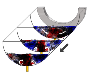
Although individual eigenmode cannot fully describe the energetic coherent structures, the structure of each eigenmode is of interest, nonetheless, as a fundamental building block of the complete structure (Liu, Adrian & Hanratty Reference Liu, Adrian and Hanratty2001). Figure 10 shows samples of the four most energetic POD eigenmodes in the cross-section at  $x/R = 0.2$ close to the orifice plate. The vectors represent the in-plane velocity components, and the background colour represents the streamwise velocity component. The red colour represents streamwise velocity larger than the local mean, and the blue colour represents streamwise velocity smaller than the local mean velocity. The broken white line represents the orifice lip's location to help identify different flow field regions. From the POD eigenmodes in figure 14, one can see a very stable potential-core region with no organized large-scale energetic motions. These POD eigenmodes demonstrate the momentum transfer between the recirculation and the shear layer regions. More specifically, the low-speed streamwise velocity (compared with the local mean velocity) is generally associated with the inward wall velocity, and the high-speed streamwise velocity (compared with the local mean velocity) is associated with outward wall velocity, which can be seen from figure 10(a–c). The noticeable azimuthal velocity will mix the high- and low-speed fluid in the recirculation region, which is probably responsible for the strong three-dimensional property of this flow field.

Figure 10. Samples of the four most energetic POD eigenmodes at  $\; x/R = 0.2$: (a) m = 1, n = 1; (b) m = 2, n = 1; (c) m = 3, n = 1; (d) m = 0, n = 1.
Figure 11 shows samples of the four most energetic POD eigenmodes in the cross-section at  $x/R = 2$. The four most energetic eigenmodes are all associated with one radial mode and 1 to 4 azimuthal modes. From these four energetic eigenmodes, we can observe that there is no longer a very stable potential-core region, especially from figure 11(d). The in-plane velocity components form counter-rotating vortex pairs, entraining low-speed velocity (compared with the local mean) fluid from the wall to the pipe centre or ejecting the high-speed velocity (compared with the local mean) fluid from the pipe centre towards the pipe wall. Note that the shape of the most energetic eigenmodes of the orifice flow at this location is similar to those of the pipe flow, as shown in Hellström et al. (Reference Hellström, Marusic and Smits2016), suggesting that the flow is beginning to recover to a pipe flow.

Figure 11. Samples of the four most energetic POD eigenmodes at  $\; x/R = 2$: (a) m = 2, n = 1; (b) m = 3, n = 1; (c) m = 4, n = 1; (d) m = 1, n = 1.
Figure 12 shows samples of the four most energetic POD eigenmodes in the cross-section at  $x/R = 4$. Figures 12(a)~12(c) show that the first three most energetic POD eigenmodes are associated with one radial mode and 1~ 3 Fourier-azimuthal modes. These basic POD eigenmodes are similar to these in the middle of the primary recirculation region at
  $x/R = 2$ as shown in figure 11(a,b,d) and those in a pipe flow. However, modal switching is very obvious, i.e. helical mode 1 becomes the most energetic eigenmode from the fourth most energetic eigenmode in the cross-section at
  $x/R = 2$. Also, the expansion of the POD eigenmodes in the radial direction can be easily seen if one compares the background contours shown in figures 11 and 12. Note that POD eigenmodes with two radial structures appear in the fourth most energetic flow patterns, probably caused by the flow redevelopment.

Figure 12. Samples of the four most energetic POD eigenmodes at  $\; x/R = 4$: (a) m = 1, n = 1; (b) m = 2, n = 1; (c) m = 3, n = 1; (d) m = 1, n = 2.
4.3. Instantaneous flow field and wall mass transfer rate
Before discussing the relationships between the large-scale energetic coherent structures and the wall mass transfer rate, we first study the variation of the instantaneous wall mass transfer rate and the velocity close to the wall mass transfer sensor. The flow field near the wall is very complicated at these three cross-sections. At this stage, it is not clear whether Taylor's hypothesis can be applied. Further, the instantaneous streamwise velocity could be either positive or negative in this reversing flow. Thus, it is difficult to determine the convection velocities of the flow structures and the wall mass transfer rate. Therefore, we directly compare the instantaneous temporal structures of the flow field and the wall mass transfer.
Figures 13–15 show the fluctuations of the wall mass transfer rate and the velocity near the wall mass transfer rate sensor at all three cross-sections for one simultaneous measurement loop. One in five points is shown to clarify the low-frequency fluctuations in these figures. Because the magnitudes of the wall mass transfer rate and velocity fluctuations are pretty different, the fluctuations are normalized by the corresponding standard deviations. Note that the velocity cannot be measured very close to the wall mass transfer rate sensor at the wall because of the resolution limit of PIV. More specifically, the closest point we can measure to the sensor locates at  $r/R = 0.96$, i.e. 0.04 R from the sensor at the wall. The wall mass transfer rate is a scalar, and its fluctuations were sampled by the circular electrode with a diameter of 1 mm. In principle, the fluctuations of all three velocity components associated with the flow structures passing by the sensor would cause the wall mass transfer rate fluctuation.
The time scales of the fluctuations of the wall mass transfer and velocity in the cross-section at  $x/R = 0.2$ (figure 13) are larger than those in the cross-sections at
  $x/R = 2$ (figure 14) and
  $x/R = 4$ (figure 15). One can observe that the low-frequency (large time scale) variation of the wall mass transfer rate could be easily related to one of the three velocity components except that there are time lags between the local peak fluctuations of the wall mass transfer rate and velocity. We believe that the concentration boundary layer develops in the electrode surface in the electrochemical method, which has a response time. Tong et al. (Reference Tong, Bhatt, Tsuneyoshi and Tsuji2020) previously discussed the time lag between the flow field and wall mass transfer rate in the electrochemical method. The time traces of the wall mass transfer rate and the velocity near the wall mass transfer rate sensor suggest that the large-scale (low-frequency) flow structures probably have footprints on the wall mass transfer rate at all three cross-sections by looking at both the time scales and the local peak values.

Figure 13. Time traces of the wall mass transfer and original velocity at the point r/R = 0.96 close to the wall mass transfer measurement sensor at  $x/R = 0.2$: all the time traces are normalized by the corresponding standard deviation, the solid black line is
  $k/\sigma (k)$; the broken green line is
  ${v_r}/\sigma ({v_r})$; the broken blue line is
  ${v_a}/\sigma ({v_a})$; and the broken red line is
  ${v_x}/\sigma ({v_x})$.

Figure 14. Time traces of the wall mass transfer and original velocity reconstructed at the point r/R = 0.96 close to the wall mass transfer measurement sensor at  $x/R = 2$: (legend is the same as that of figure 13).

Figure 15. Time traces of the wall mass transfer and original velocity reconstructed at the point r/R = 0.96 close to the wall mass transfer measurement sensor at  $x/R = 4$: (legend is the same as that of figure 13).
4.4. Spectra of the wall mass transfer rate and the velocity
To analyse the relationship between the velocity field and the wall mass transfer rate statistically, we calculate the velocity and wall mass transfer rate spectra. The spectra for both the original velocity and the velocity reconstructed by the most energetic POD eigenmodes are compared with the wall mass transfer rate spectrum. The velocity spectra for all three components are normalized by the corresponding variances and the typical time scales of the wall mass transfer rate, and the velocity spectra are averaged in the azimuthal direction. However, only the azimuthal velocity spectra are shown here for brevity because the azimuthal velocity component is the largest among the three components in the near-wall region, as shown in figures 5~7. Note that similar conclusions can be obtained for the other two velocity components, as shown in figures 23~25 in Appendix B.
Figure 16 shows the power spectra density of the wall mass transfer rate and the azimuthal velocities for different radial positions at the cross-section  $x/R = 0.2$. The original velocity spectra shown in figure 16(a) can be divided into three groups, i.e. the spectra in the core, shear layer and recirculation regions. The black and green solid lines representing the velocity spectra in the recirculation region have similar profiles. The cyan line represents the velocity in the shear layer region and has a small peak around non-dimensional frequency 20, probably the typical frequency of the vortex shedding in the shear layer region. Note that this peak is more evident in the spectra of the radial and the streamwise velocities (shown in figure 23 in Appendix B). The velocity spectra in the core and shear layer regions (the red and blue solid lines) are very different from the wall mass transfer rate spectrum (the black dashed line) since they are relatively far away from the wall mass transfer rate measurement sensor. However, velocity spectra in the recirculation region (the solid green and black lines) are similar to the wall mass transfer rate spectrum in the low-frequency region, suggesting that the low-frequency (large time scale) flow structures probably have a relationship to the wall mass transfer rate. However, the profile of the wall mass transfer spectra starts to differ from that of the velocity in the non-dimensional frequency region
  $f\Delta {t_0} > 2$.

Figure 16. Spectra of the wall mass transfer rate and azimuthal velocity for different radial positions (r/R = 1 is the pipe wall) at the streamwise position  $x/R = 0.2$: (a) wall mass transfer and original velocity; (b) wall mass transfer rate and reconstructed velocity using ten most important eigenmodes. The superscript ‘rec’ represents the reconstructed velocity.
Figure 16(b) shows the spectra of the wall mass transfer rate and the velocity reconstructed by the ten most energetic POD eigenmodes, accounting for approximately 33% of the turbulent kinetic energy. The reconstructed velocity spectra can still be divided into three groups similar to the original velocity spectra. However, noticeable differences between the original and reconstructed velocity spectra also appear. For instance, the reconstructed velocity spectra in the core and shear layer regions have small peaks around non-dimensional frequency 20, which can also be seen in the spectra for the other two velocity components shown in figure 23 in Appendix B. We assume that this frequency is related to the large-scale coherent structures in the secondary recirculation region. Although the original velocity spectra in the shear and core regions (the red, blue and cyan lines) do not agree with the wall mass transfer rate spectrum, all the spectra of the velocity reconstructed by the most energetic POD eigenmodes agree reasonably well with the wall mass transfer rate spectrum in the low-frequency region  $(f\Delta {t_0} < 2)$, especially the reconstructed velocity spectra in the recirculation region (the black and green solid lines). This result reveals that the low-frequency wall mass transfer rate fluctuation is probably related to the large-scale energetic coherent structures.
Figures 17 and 18 show the spectra of the wall mass transfer and the azimuthal velocity at the cross-sections  $x/R = 2$ and
  $x/R = 4$, respectively. The selection of different numbers of POD eigenmodes to reconstruct the velocity field is based on the energy profile of the POD eigenmodes shown in figure 9. The solid black line representing the original velocity spectrum in the near-wall region at the cross-section
  $x/R = 2$ has similar profiles to that of the wall mass transfer rate in the low-frequency region
  $(f\Delta {t_0} < 2)$ as shown in figure 17(a), which suggests that the dynamical properties of velocity field in the low-frequency region at the cross-section
  $x/R = 2$ are similar to those of the wall mass transfer rate. Additionally, the low-frequency region of the velocity spectra can be reconstructed by the large-scale energetic eigenmodes (80 modes in the present case), as shown in figure 17(b). The blue and red lines representing the original velocity spectra in the shear layer regions peak around
  $f\Delta {t_0} \approx 3$ in figure 17, which we assume is probably related to the vortex shedding property in the shear layer region. This property is more evident in the original and reconstructed velocity spectra for the radial and streamwise velocity components, as shown in figure 24 in Appendix B.

Figure 17. Spectra of the wall mass transfer rate and the azimuthal velocity at different radial positions (r/R = 1 is the pipe wall) at streamwise position x/R = 2: (a) wall mass transfer and original velocity; (b) wall mass transfer rate and reconstructed velocity using 80 most important eigenmodes. The superscript ‘rec’ represents the reconstructed velocity.

Figure 18. spectra of wall mass transfer rate and azimuthal velocity at different radial positions (r/R = 1 is the pipe wall) at streamwise position x/R = 4: (a) wall mass transfer and original velocity; (b) wall mass transfer rate and reconstructed velocity using 50 most important eigenmodes. The superscript ‘rec’ represents the reconstructed velocity.
One can also observe from figure 18(a) that the solid black line representing the original velocity spectrum in the near-wall region at the cross-section  $x/R = 4$ agrees with the wall mass transfer spectrum in the low-frequency region
  $(f\Delta {t_0} < 2)$. Moreover, this spectrum can be reconstructed by the large-scale energetic POD eigenmodes if one compares figures 18(a) and 18(b). Note that the red and blue lines in figure 18(a), representing the original azimuthal velocity spectra, show a small peak around
  $f\Delta {t_0} \approx 2$, which can also be seen in the original radial velocity spectra in figure 25 in Appendix B. However, the original streamwise velocity spectra do not have this peak. We assume that this peak is probably related to the shear layer reattachment process.
We find out from the above discussions that the wall mass transfer rate spectra agree reasonably well with the spectra of velocity reconstructed by the most energetic eigenmodes in the low-frequency region at all three specific cross-sections. We thus assume that the large-scale energetic coherent structures’ frequency properties are related to those of the wall mass rate. In other words, the energetic coherent structures are probably related to the low-frequency variation of the wall mass transfer rate in the near field of orifice flow.
4.5. Stochastic estimation of the flow field associated with large wall mass transfer rate
Figure 19 shows the quadratic stochastic estimation of the conditionally averaged flow field associated with the large wall mass transfer rate  $(k > 5 \; {k_{rms}})$ at all three cross-sections, where k is the wall mass transfer rate fluctuation and
  ${k_{rms}}$ is the root mean square of the fluctuation. One can observe from figure 19(a) that large-scale azimuthal velocity patterns with opposite directions appear in the conditionally averaged flow field. In addition, the background contour shows the high-speed fluid flanked by low-speed fluid. If we compare figure 19(a) with the samples of the several most energetic POD eigenmodes shown in figure 10, we can observe that the first three most energetic POD eigenmodes show similar velocity patterns. The difference is that the scale of the velocity patterns in the azimuthal direction may be different. Figures 19(b) and 19(c) show similar counter-rotating vortex pairs in the conditionally averaged velocity fields associated with large wall mass transfer rates. All the most energetic POD eigenmodes at the cross-sections
  $x/R = 2$ and
  $x/R = 4$ show counter-rotating vortex pairs of different radial and azimuthal scales. In addition, the distribution of the streamwise velocity shown as the background contour is also similar. More specifically, there are high-speed regions flanked by low-speed regions for both cross-sections. We believe that comparing the stochastic estimation results in figure 19 and the most energetic POD eigenmodes reveals evidence of the strong effects of the large-scale energetic coherent structures on the wall mass transfer rate at all three specific cross-sections in the near field orifice flow. Note that the counter-rotating vortex pairs enhancing the wall mass transfer rate here in figures 19(b) and 19(c) are very similar to the flow structures enhancing the wall shear stress (Tong et al. Reference Tong, Bhatt, Tsuneyoshi and Tsuji2020) in a pipe flow and the sketch of large-scale coherent flow motions in the boundary layer of wall-bounded flow (Marusic, Mathis & Hutchins Reference Marusic, Mathis and Hutchins2010).

Figure 19. Stochastic estimation of the conditionally averaged flow structures associated with large wall mass transfer rate at: (a) cross-section x/R = 0.2; (b) cross-section x/R = 2; (c) cross-section x/R = 4.
5. Conclusions
Although the flow fields away from the wall at three specific locations behind the orifice plate are quite different, the wall mass transfer rate spectra collapse in the low-frequency region, suggesting that the low-frequency wall mass transfer rate probably follows the same physics in orifice flow. The instantaneous traces of the wall mass transfer rate and velocity near the wall mass transfer sensor suggest that the instantaneous flow structures probably have footprints on the wall mass transfer rate, although time lags exist due to the response of the concentration boundary layer. Additionally, the collapse of the spectra of the velocity reconstructed by the most energetic eigenmodes and the wall mass transfer in the low-frequency region at all investigated three specific locations reveals that the large-scale energetic eigenmodes are related to the low-frequency wall mass transfer rate fluctuation. Furthermore, comparing the most energetic POD eigenmodes and the stochastic estimation results of conditionally averaged velocity fields associated with large wall mass transfer at all three specific locations suggests that the large-scale energetic coherent structures are strongly related to the wall mass transfer rate enhancement. This finding indicates that it is possible to control the large-scale coherent structures to reduce FAC and prevent pipe ruptures in the industry.
Funding
We acknowledge the National Natural Science Foundation of China (Grant No. 51606073, 51736004) and the Double first-class research funding of the China-EU Institute for Clean and Renewable Energy.
Declaration of interests
The authors report no conflict of interest
Appendix A. Validation of the experimental results
Figure 20 shows the instantaneous streamwise velocity measured by the CCD cameras under the original Cartesian and interpolated cylindrical coordinate systems, respectively. We can observe no apparent difference between the original velocity field and the interpolated original velocity field, excepting small flow structures in the lower right corner introduced by the interpolation. However, the present study focuses only on large flow structures. Therefore, it is reasonable to assume that the interpolation adopted in the present study is reliable.

Figure 20. Instantaneous streamwise velocity under the original Cartesian (a) and interpolated cylindrical (b) coordinate systems at the cross-section  $x/R = 2$.
Figure 21 compares statistical quantities obtained by low-speed and high-speed PIV systems using a different number of snapshots. We use the normalized streamwise velocity as an example of the statistical quantities, the solid lines represent data from the low-speed PIV system, and the broken lines represent data from the high-speed PIV system. We can see negligible discrepancies between the profiles using 1500 low-speed snapshots and all snapshots of low-speed PIV. Therefore, we conclude that we obtain converged statistics using the low-speed PIV data. However, we observe apparent discrepancies in the statistical quantities among different snapshots of high-speed PIV. Moreover, there are noticeable discrepancies among the profiles of low-speed and high-speed PIVs, suggesting that the high-speed PIV's first-order quantities are not convergent.

Figure 21. Comparison of mean streamwise velocity using a different number of snapshots from both low-speed and high-speed PIV systems at  $x/R = 4$.
Figure 22 shows the uncertainty of PIV in our measurement at the cross-section at  $x/R = 0.2$ as an example. We select this location because the turbulent intensity and the velocity gradient are significant in the shear layer region at this cross-section, which decreases the measurement accuracy. From figure 7, we can observe that significant uncertainties exist in the shear layer region for both the statistical and time-resolved PIV measurement. However, the results are still acceptable because the velocity itself is large (usually larger than 1 m s−1, as we can see from figure 8).

Figure 22. Root mean square of streamwise velocity's uncertainty at the cross-section  $x/R = 0.2$: (a) statistical PIV; (b) time-resolved PIV.
Appendix B. Comparison of the spectra of the velocity and wall mass transfer rate
Figures 23–25 show the power spectra density of the wall mass transfer rate and the velocity for different radial positions at all three cross-sections, respectively. The comparison of original and reconstructed velocity spectra for the azimuthal component is presented in § 4.4. The comparison of original and reconstructed velocity spectra for the radial and streamwise velocity components is shown in here.

Figure 23. Spectra of wall mass transfer rate and velocity at different radial positions (r/R = 1 is the pipe wall) at streamwise position x/R = 0.2.

Figure 24. Spectra of wall mass transfer rate and velocity at different radial positions (r/R = 1 is the pipe wall) at streamwise position x/R = 2.

Figure 25. Spectra of wall mass transfer rate and velocity at different radial positions (r/R = 1 is the pipe wall) at streamwise position x/R = 4.


