Methodology and data

In this study the Optimum Multiparameter (OMP) analysis was applied to quantify mixing between the major water masses present in the Weddell Sea intermediate and deep layers. Due to the high surface variability, only layers below 500 m were analysed. Thus, only the deepest WDW, which mixes with less dense WSDW, is analysed here. The OMP analysis is based on the supposition that water mass mixing is linear and affects all parameters equally (Tomczak & Large Reference Tomczak and Large1989). Below we briefly describe the fundamental concepts for the analysis.

A water mass is defined as a physical entity that occupies a finite volume in space (Tomczak & Large Reference Tomczak and Large1989) or as a body of water with a common formation history and source in a specific area of the ocean (Tomczak Reference Tomczak1999a). The water type is defined as a set of parameters which describe the water mass properties and is thus an artificial construction without any real volume in space (Tomczak & Large Reference Tomczak and Large1989). Although this study investigates one of the main AABW source regions (i.e. the Weddell Sea), it is out of our scope to identify source waters contributions (i.e. shelf waters). Therefore, our studies rely on definitions of local water masses (i.e. water types instead of source water types) as in Tomczak & Liefrink (Reference Tomczak and Liefrink2005) and Kerr et al. (Reference Kerr, Wainer and Mata2009). The aspects of water masses variability and changes that fulfil the Weddell deep water column following the Weddell Gyre circulation are also discussed here.

The available number of hydrographic parameters limits the number of water types that can be used with the OMP method. Only two physical restrictions are imposed in the OMP analysis: first, mass conservation, i.e. the contribution of all water types has to amount to 100%, and secondly, a particular water mass contribution cannot be negative. A detailed description of advantages and other applications of the method can be obtained from Tomczak & Large (Reference Tomczak and Large1989), Karstensen & Tomczak (Reference Karstensen and Tomczak1997), Poole & Tomczak (Reference Poole and Tomczak1999), and Kerr et al. (Reference Kerr, Wainer and Mata2009). OMP analysis has an advantage over the mixing triangle because it includes a non-negativity constraint, which gives another degree of freedom and allows an optimization process (M. Tomczak, personal communication 2006).

The following water masses were chosen to be quantified by OMP in the deep layers of the Weddell Gyre oceanic regime: WDW, WSDW, and WSBW. In order to calculate water type index for each water mass, the approach based on the choice of the most pure form of particular water mass was applied. Using the Weddell Sea data available at the US National Oceanographic Data Center (NODC/NOAA), hydrographic stations of specific areas (Fig. 2) and depths (Table I) were selected to represent regions where each of the chosen water masses appear to be unadulterated. The inflowing water type (i.e. WDW) is defined along the Weddell Gyre eastern limb at the transition between the ACC and the gyre, where its initial characteristics are set. Observations in the Weddell–Enderby basin represent recently formed WSDW and WSBW masses adequately. This approach presents a certain degree of subjectivity in the water masses definitions. However, both the year to year variability and the influence of other water masses are minimized. A typical θ/S diagram for the study area is shown in Fig. 3.

Fig. 2 NODC/NOAA stations selected to calculate the water type indices. The time period of sampling considered here is from 1963 to 1996. The years in parentheses are used for each water mass: WDW (▵ = 1977, 1981, 1985, 1988, 1993), WSDW (□ = 1968, 1969, 1985, 1989, 1990, 1992, 1996) and WSBW (● = 1963, 1964, 1966–69, 1973, 1975, 1977, 1981, 1984, 1985, 1987–90, 1992, 1993, 1996). The depths considered for each water mass are listed in Table I.

Table I Selected depth and θ range used to calculate the water type index.

Fig. 3 Typical θ/S diagram for the study area in Weddell Sea (WOCE SR4). The solid line, dashed lines, and dotted line show, respectively, the σ₀, σ₂, and σ₄ contours. The boxes indicate the thermohaline limits for each water mass considered.

The θ range (Table I) used in the linear regression to calculate the salinity and dissolved oxygen (DO) values are based on Robertson et al. (Reference Robertson, Visbeck, Gordon and Fahrbach2002). DO is widely used to delineate water mass distribution (Emery & Thomson Reference Emery and Thomson1998) and acts as a conservative chemical tracer in the Antarctic deep ocean because its consumption is below its detectable limit. The DO values were converted to μM (i.e. μmol L^-1), in accordance with the equation described by Weiss (Reference Weiss1981). Table II shows the water type index parameters (i.e. θ, salinity, and DO) considered in this work to represent the selected water masses and their respective weights used as model input.

Table II Water type definitions, parameter errors used for perturbed models, and parameter weight used for OMP model input. The parameters used are: Potential temperature (θ), Salinity, and Dissolved Oxygen (DO). The δ_max corresponds to each parameter maximum variance.

Resolving water masses within a small range of parameter values depends on correct weighting of the parameters (J. Karstensen, personal communication 2007). The weights applied here were calculated in accordance with the variance equation described by Tomczak & Large (Reference Tomczak and Large1989), which uses the variance of the water types and the highest variance (δ_max) found in the source area for each parameter. Thus, our analyses were restricted to the deep ocean below 500 m, a depth range where homogeneous weights might apply.

The majority of the datasets used in this study were obtained from the World Ocean Circulation Experiment (WOCE) programme database. WOCE SR4 and Greenwich Meridian repeat hydrographic sections (Fig. 1) were selected for their relatively high number of repetitions. The WOCE SR4 dataset covers the Weddell Sea central region from the Antarctic Peninsula (∼63°W) to Kapp Norvegia (∼13°W) with several repeats between 1989 and 1998 (i.e. October 1989, December 1990, December 1993, April 1996, April 1998, available at http://whpo.ucsd.edu/). The 1998 dataset consists only of the western portion of the WOCE SR4 section. The Greenwich data were obtained from NODC/NOAA historical dataset with repeats between 1984 and 1998 (i.e. February 1984, December 1986, June 1992, April 1996, May 1998; available at http://www.nodc.noaa.gov/). Some of them represent the southern portion of the section WOCE A12.

OMP output data (i.e. the water mass contributions) was optimally interpolated onto a regular longitude/latitude pressure grid (i.e. 0.1°-10 m). Differences between the water mass contribution of each year and the mean contribution for the same water mass from all cruises were computed at each grid point to calculate the water mass anomalies for the respective years. The water mass anomalies were standardized with respect to the standard deviation of the mean field. Anomalies were calculated only if the percentage of water mass contribution to the mixture was greater than 30%.

Sensitivity analysis

Sensitivity analyses were performed on the OMP outputs to assess the quantitative validity of the results. The OMP outputs are considered to be qualitatively valid due to the continuity of the water mass spatial distributions along the entire water column, in agreement with the expected distribution based on the observed fields. A more quantitative validation of the results is needed to verify the sensitivity of the water mass contributions to different error sources, such as instrumental and analytical precision, environmental variability, and variations associated with the water type definition. The latter is an important issue because variability identified by the analysis method in water mass contributions to the total mixture could also arise from temporal variability. It may not be possible to distinguish between the two. As noted in the methodology section, OMP analysis assumes that no temporal change in source waters. Thus, the variability of the water mass contributions could, in part, be artefacts of the method instead of real variations in water mass fractions.

To tackle this question and provide a more quantitative assessment of the results, we performed a sensitivity analysis by perturbing the defined water types by adding or subtracting standard errors on the parameters, estimated from local water type definitions (see Table II). Water mass composition is marginally modified by changes in the water type definitions (not shown). Since the deviation of the conservation of mass residuals is negligible in comparison to the uncertainties of water mass fractions, an increasing contribution of one water mass is accompanied by a drop of the others. In summary, the analysis has produced reasonable dense water mass distributions in the Weddell Sea that are supported by the low residuals of mass conservation, which do not exceed 5%, for all years considered. There is a good match between the water types applied and the historical dataset used for all cruises.

Several earlier studies addressed the temporal evolution of Weddell Sea water masses over a period that is covered by the dataset presented here. These works all identify a linear warming trend of 0.012°Cyr^-1 for WDW and 0.01°C yr^-1 for WSBW (Robertson et al. Reference Robertson, Visbeck, Gordon and Fahrbach2002, Fahrbach et al. Reference Fahrbach, Hoppema, Rohardt, Schröder and Wisotzki2004). Thus it is of interest to investigate how a non-static temperature history may affect the present work.

A sensitivity test is performed to show how the fractional water mass contributions might change if a time-dependent temperature is used. A linearly raising function (Eq. 1) is applied to correct the θ index of WDW and WSBW for each year (t_obs). Slightly different water types () are used in this calculation for each year because changes in the properties of the water types also emerge as variations of the fractional composition in the mixture (Leffanue & Tomczak Reference Leffanue and Tomczak2004). As no significant trend was determined for WSDW by Robertson et al. (Reference Robertson, Visbeck, Gordon and Fahrbach2002), we have maintained the WSDW index. In the same sense, as temporal salinity and DO variations are not clearly identified for the Weddell Sea, only the θ index for WDW and WSBW were changed in this test. In general, the typical water type variability does not impose significant errors in the overall results, thus temporal changes of source water properties are not the only cause of the observed water mass contributions variations. More details on deep water mass variability are explained in the following section.

(1)

Weddell Sea water masses structure

Water mass stratification obtained with our OMP analysis is in general agreement with the distribution based on hydrographic ranges as suggested by others (Carmack & Foster Reference Carmack and Foster1975, Fahrbach et al. Reference Fahrbach, Rohardt, Schröder and Strass1994, Reference Fahrbach, Hoppema, Rohardt, Schröder and Wisotzki1995, Reference Fahrbach, Rohardt, Scheele, Schröder, Strass and Wisotzki2004, Klatt et al. Reference Klatt, Fahrbach, Hoppema and Rohardt2005, Smedsrud Reference Smedsrud2005). Figures 4 & 5 show, respectively, the water mass mean distribution and contribution during the 1990s in the Weddell Sea and the associated standard deviation. At the WOCE SR4 section, WDW is present in an intermediate layer down to 1500 m, reaching a contribution of 30% (Fig. 4a). WSDW core is present at greater depths, with a highest contribution of> 70% between 1500–3500 m (Fig. 4c), whereas WSBW is restricted to the near-bottom, below 4000 m (Fig. 4e). The mean water mass distribution and contribution at the Greenwich Meridian shows that WDW reaches contributions around 30–50% in depths between 1500–2000 m (Fig. 4b). WSDW contributes with around 50–70% in depths between 1000–3500 m (Fig. 4d), while WSBW is constrained to the region north of Maud Rise (64–67°S) with a highest contribution of> 70% (Fig. 4f).

Fig. 4 Weddell Deep Water masses mean contribution (%) at the WOCE SR4 (left) and Greenwich Meridian (right) sections, respectively, a, b. WDW, c, d. WSDW, e, f. WSBW.

Fig. 5 Standard deviation of Weddell Deep Water masses mean contribution (%) at the WOCE SR4 (left) and Greenwich Meridian (right) sections, respectively, a, b. WDW, c, d. WSDW, e, f. WSBW.

Our analysis of the WOCE SR4 section shows WSDW and WSBW isolines tilted towards the western continental shelf (Fig. 6), which reflects the proximity to source waters. Furthermore, high levels (> 50%) of WSBW contribution are found along the north-western slope (Fig. 4e) identifying the western Weddell Sea as a source region for newly formed bottom water. However, noble gas observations taken along drift tracks parallel to the Antarctic Peninsula has showed that high WSBW fraction attached to the slope are fed by sources of the southern Weddell Sea (e.g. from the region near the Filchner–Ronne Ice Shelf) and also by local sources along the Antarctic Peninsula (Weppernig et al. Reference Weppernig, Schlosser, Khatiwala and Fairbanks1996, Huhn et al. Reference Huhn, Hellmer, Rhein, Rodehacke, Roether, Shodlock and Schröder2008). Although only the layers below 500 m were considered in this work, the WDW distribution exhibits a deepening next to the Antarctic coastline near to Kapp Norvegia in the WOCE SR4 section (Fig. 4a), which is possibly linked to the easterly winds causing surface Ekman flux to be southwards and hence driving coastal downwelling.

Fig. 6 Weddell Deep Water masses contribution (%) along the WOCE SR4 section during each repeat cruise. Columns indicate WDW (1st), WSDW (2nd), and WSBW (3rd) contributions. Each row corresponds to a particular year (or cruise) as indicated in the first box.

The water mass distribution and contribution (Figs 6 & 7) to the observed mixture shows high temporal variability at all levels (Kerr Reference Kerr2006). That is particularly true for WSBW layers when extreme years can be readily observed, like 1990 and 1996 for the WOCE SR04 section (Fig. 6l & n). The same layers in the Greenwich section exhibit a steady decrease of the contribution of WSBW between 1984 and 1998 (Fig. 7k–o). The WDW pattern is less variable, especially in WOCE SR04 section approximately along the centre of the Weddell Gyre. Lower variability would be expected at this location. Generally, the degree of variability is similar for both WSDW and WSBW but with opposite trends.

Fig. 7 Weddell Deep Water masses contribution (%) along the Greenwich Meridian section during each repeat cruise. Columns indicate WDW (1st), WSDW (2nd), and WSBW (3rd) contributions. Each row corresponds to a particular year (or cruise) as indicated in the first box.

The mean water mass contribution is calculated for defined depth intervals, which should embrace the water mass core, i.e. WDW between 500–700 m, WSDW between 1500–3000 m, and WSBW below 4000 m. An increasing (decreasing) trend in the WDW (WSBW) contribution is identified for both sections analysed (Fig. 8). In addition, the decrease of WSBW contribution along the Greenwich Meridian section would coincide with the decrease in the central Weddell Sea (i.e. WOCE SR4 section) starting roughly two years earlier. It is important to note, however, that sampling frequency can affect the apparent timing of the events. The earlier decrease of WSBW along the central Weddell Sea might be an artefact of sampling frequency. Although the WSDW contribution behaviour is slightly different for the two sections considered, the trends reported for both sections can also be associated with different sampling frequencies. While WSDW contribution remains relatively constant in the WOCE SR4 section, there is an increasing trend in the Greenwich Meridian section after 1984. A similar pattern was found by Fahrbach et al. (Reference Fahrbach, Hoppema, Rohardt, Schröder and Wisotzki2004) who estimated the variability of the area occupied by the Weddell Sea water masses along both transects. The main patterns of trends in fractional water mass contribution identified with the evolving temperature analysis do not change the main pattern for either section. However, only slight changes in water masses contribution are observed (Fig. 8c, d, f).

Fig. 8 Time series of the mean contribution to the total mixture (%) in the core of the water mass for a.–d. WOCE SR4, e. & f. Greenwich Meridian sections. When 1998 data is included only the western portion of the WOCE SR4 section is considered (b, d). The following depth intervals were used: WDW (500–700 m), WSDW (1500–3500 m), and WSBW (> 4000 m). The mean contributions were calculated using water types from Table II (a, b, e) and varying the water types (c, d, f) as indicated in the text.

The 1998 results, particularly for the WOCE SR4 section, stand apart from others reported here. The section was occupied far away from the inflow of WDW and close to sources of WSBW. So the results are probably biased towards the WSBW outflow, which may in turn bias the mean contributions identified in our analysis. To verify how all the fractions along this section evolve in time, restrict the analysis to cruises onto the western part only. During this specific year, all layers show a marked change in the trend for WOCE SR4 section (Fig. 8b) which is not observed in the Greenwich Meridian region.

The 1984 Greenwich Meridian section analysis yields an anomalous WSDW distribution evidenced by the related upward shift of the thin WSDW layer (Fig. 7f). The shift probably extends into 1986. Gordon (Reference Gordon1978) reported open-ocean convection during the 1970s in the vicinity of the Greenwich Meridian section. However, although Klatt et al. (Reference Klatt, Roether, Hoppema, Bulsiewicz, Fleischmann, Rodehacke, Fahrbach, Weiss and Bullister2002) do not identify any signature attributed to convective events through the analyses of CFC data, those authors show a mid-depth CFC minimum layer for that particular year. The anomalous distribution of WSDW showed through OMP results occupies the same ocean layer where Klatt et al. (Reference Klatt, Roether, Hoppema, Bulsiewicz, Fleischmann, Rodehacke, Fahrbach, Weiss and Bullister2002) identified the lower CFC values. The anomaly may indicate that source waters properties resulted in denser waters, as evidenced by the high contribution of WSBW for this specific year (Fig. 7k).

Warm deep water variability

Variations in WDW distribution are relatively subtle between 1984 and 1998 (Figs 6a–e & 7a–e). However, with the exception of 1998, the WDW contribution anomalies increase overall during this period (Figs 9a–e & 10a–e) as can be observed also for the contribution of the water mass core (Fig. 8). Because only the water column below 500 m was considered, part of the intermediate water column was not analysed. The increase of WDW contribution is consistent with the water temperature increase reported for the same period (Fahrbach et al. Reference Fahrbach, Hoppema, Rohardt, Schröder and Wisotzki2004). Hence, the observed increase may result from both the intensification of WDW inflow into the Weddell Sea and warming of the intermediate layer (i.e. WDW itself is getting warmer). Warming is consistent with observations that globally the largest oceanic heat variability during the last fifty years occurred in the upper 700 m of the ocean (Levitus et al. Reference Levitus, Antonov and Boyer2005). Gille (Reference Gille2002) showed a warming trend of ∼0.01°C yr^-1 of southern waters for the 700–1100 m depth range between 1950 and 1980, while Aoki et al. (Reference Aoki, Yoritaka and Masuyama2003) indicated a similar sub-surface warming for the southern ACC region. Robertson et al. (Reference Robertson, Visbeck, Gordon and Fahrbach2002) and Smedsrud (Reference Smedsrud2005) also reported a WDW heating of ∼0.012°C between 1975 and 2001. The increase of the intermediate water temperatures for the Southern Ocean is associated with the rising temperature trend of the global ocean (Levitus et al. Reference Levitus, Antonov, Boyer and Stephens2000). However, Fahrbach et al. (Reference Fahrbach, Hoppema, Rohardt, Schröder and Wisotzki2004) suggest that this period of warming is finished, therefore, their observations point to a reduction of the average temperature after the 1990s, indicating the beginning of a cooling period for this layer. In fact, the decreasing of WDW core contribution for 1998 (Fig. 8) may be associated with those changes in temperature. Gordon (Reference Gordon1982) showed WDW temperatures slightly cooler for the period from 1973 to 1977 west of the Greenwich Meridian related to the occurrence of the Weddell polynya. Thus, the current changes in ocean temperature may indicate natural variability on decadal time scales. The details of such variations are still a matter of intense debate (e.g. Aoki et al. Reference Aoki, Rintoul, Ushio, Watanab and Bindoff2005). Long-term studies within a sensitive area like the Weddell Sea are required to address this subject, in particular, to separate the anthropogenic induced changes from the natural variability.

Fig. 9 Weddell Deep Water masses contribution anomalies along the WOCE SR4 section for a.–e. WDW, f.–j. WSDW, k.–o. WSBW. Each row corresponds to a particular year (or cruise) as indicated in the first box. The units are point-wise normalized and represent the number of standard deviations from the overall mean.

Fig. 10 Weddell Deep Water mass contribution anomalies along the Greenwich Meridian section for a.–e. WDW, f.–j. WSDW, k.–o. WSBW. Each row corresponds to a particular year (or cruise) as indicated in the first box. The units are point-wise normalized and represent the number of standard deviations from the overall mean.

Fahrbach et al. (Reference Fahrbach, Hoppema, Rohardt, Schröder and Wisotzki2004) pointed to remote and local processes that could be involved in the observed WDW warming. Those authors believe that the main forcing on WDW variability is large-scale processes originating outside the Weddell Gyre. These changes together might cause the WDW variability quantified here (Figs 9a–e & 10a–e). The main external mechanisms which could explain the WDW warming and, consequently, the variability of WDW distribution and contribution relate to changes in CDW transport to the Weddell Sea. A greater injection of CDW could be due to ACC instabilities near the Weddell Front and the northern limb of the Weddell Gyre (the Southern Boundary of the ACC is sketched in Fig. 1; see Orsi et al. Reference Orsi, Whitworth and Nowlin1995) or to ACC intensification at the eastern limb of the gyre (20–30°E). A westward displacement of the atmospheric mean low sea-level pressure provides more favourable conditions for a CDW inflow (Fahrbach et al. Reference Fahrbach, Hoppema, Rohardt, Schröder and Wisotzki2004). Thus, the increase of the WDW contribution to the Weddell Sea reported in this work (Fig. 8) is probably related to the atmospheric and oceanic processes described above.

A better understanding of the causes of WDW variability is also essential to understanding bottom water variability. As WDW is one of the source water masses for deep and bottom water in this region, alterations in intermediate layer properties are likely to propagate and to be linked to changes in WSBW characteristics. Aoki et al. (Reference Aoki, Rintoul, Ushio, Watanab and Bindoff2005) showed that Antarctic–Australian Basin bottom water cooled (∼0.2°C) and freshened (∼0.03) over the last 10 years. However, determining the time scales of water mass formation processes (i.e. atmospheric and oceanic processes) and the fraction of WDW that finally enters in recently formed WSBW is difficult.

Coupled oceanic-atmospheric variability in the Weddell Sea

In order to understand the internal variability of the Weddell Sea, the complex links between atmospheric processes and changes with the ocean - such as sea ice variations, brine release, and source water masses involved in dense water formation - must be tackled. The different temporal scales of sea ice cycles, oceanic and atmospheric responses add challenges to reaching that goal. To gain insight into the variability observed in the water masses described in this study, correlations between bottom water mass temporal anomalies and modes of atmospheric and oceanic variability are explored in the following subsections.

Southern Annular Mode (SAM)

The Southern Hemisphere atmospheric circulation is characterized by a circumpolar vortex that extends from the surface to the stratosphere. The variability of the vortex is dominated by what is known as Antarctic Oscillation, High Latitude Mode, or Southern Annular Mode (SAM; Thompson & Wallace Reference Thompson and Wallace2000). The SAM index defined by Gong & Wang (Reference Gong and Wang1999) is used throughout this study. Those authors define the SAM index as the difference of the zonal mean sea level pressure between 40°S and 65°S. Visbeck & Hall (Reference Visbeck and Hall2004) shown that the SAM is represented by the first empirical orthogonal function in the 850 hPa pressure surface, accounting for ∼20% of the total variance. Several studies highlight the importance of the SAM for the ocean variability and sea ice fluctuations over distinct time scales (e.g. Hall & Visbeck Reference Hall and Visbeck2002, Liu et al. Reference Liu, Curry and Martinson2004, Simmonds & King Reference Simmonds and King2004). Recently, a positive trend in the SAM index has been observed (Fig. 11a), which tends to enhance the circumpolar vortex and intensify westerlies around the Antarctic continent (Marshall Reference Marshall2003).

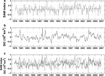
Fig. 11 Southern Annular Mode (SAM) and Sea Ice Concentration anomaly (SIC) indices. a. SAM index (grey line) between 1979–2006, black line indicates the SAM index trend. b. Monthly SIC index for the Weddell Sea sector during 1979–2006. Data from the US National Snow and Ice Data Centre (http://www.nsidc.org). c. Overlay of the SAM (grey line) and SIC indices (black line) spanning from 1979–2006.

SAM and the WSBW anomalies

A good correlation has been intensified between the SAM and ACC transport variability (e.g. Meredith et al. Reference Meredith, Woodworth, Hughes and Stepanov2004) and between the SAM and the sea ice variability (e.g. Kwok & Comiso Reference Kwok and Comiso2002, Liu et al. Reference Liu, Curry and Martinson2004). Both ACC and sea ice play an important role in the processes responsible for dense water formation within the Weddell Sea, thus a correlation between WSBW anomalies and a positive SAM index should be expected because WSBW has been recently ventilated. Hence, we expect to find a correlation between the SAM and WSBW formation trends identified by our analysis.

During positive SAM index phase, open water conditions in the Weddell Sea should facilitate new sea ice formation and thus intensify the production of dense shelf waters (Timmermann et al. Reference Timmermann, Hellmer and Beckmann2002). The intensified ACC will also cause instabilities in the Weddell Front, enhancing the injection of CDW/WDW into the Weddell Gyre (Fahrbach et al. Reference Fahrbach, Hoppema, Rohardt, Schröder and Wisotzki2004). Furthermore, modelling studies indicate that during a positive SAM index WDW upwelling is enhanced, destabilizing the water column due to an increase in the surface density (Lefebvre & Goosse Reference Lefebvre and Goosse2005). As a result, denser source waters become available and the process involved in WSBW formation is intensified. The mechanisms which link the SAM and WSBW variability are summarized in Fig. 12.

Fig. 12 Relationship scheme between the Southern Annular Mode (SAM) and WSBW contribution and/or production.

Time lag between oceanic and atmospheric processes

Antarctic sea ice variations depend strongly on the seasonal variability of atmospheric temperatures. The sea ice concentration anomalies (SIC) for the Weddell Sea sector (i.e. the same sector defined by Cavalieri & Parkinson Reference Cavalieri and Parkinson2008) may result from successive openings and closings of the sea ice cover. This is due to the gradients generated during the sea ice movement induced by advective processes and sea ice formation and melting. Thus, negative and positive SIC indicate, respectively, low and high sea ice concentration or thin and thick sea ice covers (Kwok & Comiso Reference Kwok and Comiso2002). Figure 11b shows the SIC index used in the present work for the Weddell Sea sector (extracted from the National Snow and Ice Data Center database).

Sea ice extent and drift speed are sensitive to the main Southern Hemisphere modes of variability, including the SAM (Yuan Reference Yuan2005). Both seasonal and interannual variability in sea ice cover impact surface water masses (Comiso & Gordon Reference Comiso and Gordon1998) and thus formation and export of dense waters from Antarctic seas. With the expected correlation in mind, we compute a coherence function for the SAM and SIC that may be used as a proxy in further analysis of links between atmospheric variability and WSBW formation.

High coherence values between the SAM and the SIC time series occur at several time scales (Fig. 13). The SAM influences the sea ice cover on intra-seasonal (5–7 months), annual (10–15 months), and longer (3–6 years) scales. In addition, a nearly immediate response (∼2 months) of the sea ice conditions to SAM forcing is also observed. The latter agrees with the results of Yuan (Reference Yuan2005). Cross-correlation between the SAM and the SIC indices yields decadal time scales which are particularly important to this study (∼10 yr; Fig. 14).

Fig. 13 Coherence functions between the SAM and the SIC indices. Annotations indicate periods in months corresponding to each peak. Dashed line indicates significance level above 95%.

Fig. 14 Lagged cross-correlation function between the SAM and the SIC indices (SIC lags SAM; grey line). Dashed line indicates significance level above 40%. Annotations indicate the periods in years.

The SIC may be used as an index to determine the temporal lag that exists between atmosphere forcing and the ocean surface response. If the age of the WSBW could be estimated, one could correlate the WSBW characteristics during the formation period with ocean surface conditions during that time, represented here by the SIC index. Newly ventilated WSBW is linked to sea ice processes and its variability should thus reflect SAM time scales to a certain degree.

Weddell Sea Bottom Water formation periods

Bottom water masses used in this study are not restricted to source areas only. Thus, it is necessary to estimate the SAM index during appropriate WSBW formation periods. This, in turn, requires knowledge of when the waters present at the bottom of the Weddell Sea in a given cruise were last at the surface. Water mass age can be estimated using the advanced OMP analysis tools (Karstensen & Tomczak Reference Karstensen and Tomczak1997). Unfortunately, parameters needed for those tools, such as dissolved nutrients and potential vorticity are not considered as good tracers for Antarctic waters (Thompson & Edwards Reference Thompson and Edwards1981, Tomczak Reference Tomczak1999b). Additionally, nutrient and other chemical data is not widely available for the Southern Ocean.

Several studies using transients (i.e. CFC) and radioactive (i.e. tritium) tracers indicate that during the period analysed the WSBW age varied from 10 to 15 years (see Schlosser et al. Reference Schlosser, Bullister and Bayer1991, Mensch et al. Reference Mensch, Simom and Bayer1998, Klatt et al. Reference Klatt, Roether, Hoppema, Bulsiewicz, Fleischmann, Rodehacke, Fahrbach, Weiss and Bullister2002, Huhn et al. Reference Huhn, Hellmer, Rhein, Rodehacke, Roether, Shodlock and Schröder2008). It is known that bottom waters near the continental shelves are younger than those in the interior of the gyre. Thus, we consider two time windows, 1975–80 and 1981–86, which are related with the WSBW observed in the 1990 and 1996 cruises, respectively (Fig. 15). One can expect that the water observed in the bottom of the Weddell Sea during those cruises was located very near its formation area in the time windows considered.

Fig. 15 The SAM index (black line) and time-windows (grey rectangles) from 1975–80 and 1981–86, related to WSBW formation periods of the waters observed during the WOCE cruises of 1990 and 1996, respectively.

The 10 to 15 year period estimated from the tracer analysis is in agreement with decadal time lag linking atmospheric (by the SAM index) and ocean surface processes (by the SIC index) (Fig. 14). Conversely, high correlation between the SAM and the SIC with time-lag periods of 4.3, 5.3, and 6.6 years should be more related with the residence time of approximately five years for dense water masses on the western Weddell continental shelf (Schlosser et al. Reference Schlosser, Bullister and Bayer1991, Mensch et al. Reference Mensch, Simom and Bayer1998). Thus, the WSBW variability in the Weddell deep basin seems to be correlated with close to decadal periods discussed above.

Another indication for this relationship is found between the SAM index gradient (i.e. changes from negative to positive indices) and the WSBW positive anomalies (Fig. 15). From the available data, strong positive SAM gradient is associated with the positive WSBW contribution anomaly observed in 1990, which corresponds to the 1975–80 formation periods. Times of WSBW retreat (like 1996) are preceded by periods without such trends in the SAM index (1981–86 formation periods).

Summary and conclusions

Based on the deduced temporal variability of the water column’s fractional composition, we reveal for the first time the temporal evolution of Weddell Sea Deep Water mass composition along both WOCE SR4 and Greenwich Meridian sections confirming the analysis of the general layering of the water column. Mean and annual distributions derived using OMP analysis is in agreement with several hydrographic observations in this area of the Southern Ocean. The application of OMP method reveals that WDW occupies the intermediate layer down to ∼1000 m with contribution higher than 70% of the total mixture. At the deep layer between 1500–3000 m, the analysis finds WSDW with contributions higher than 70%, except at the prime meridian where that depth interval spans 1500 to 2500 m. As for the densest water mass present in the Weddell Sea, WSBW fills the ocean basin below 4000 m with contributions higher than 70%. In addition, the waters that form WSBW hug the western continental slope as they flow downward towards the abyss.

Taking advantage of repeat hydrographic sections in the Weddell Sea during the WOCE period, we investigated the deep water mass structure and variability which showed significant changes in the water mass contribution and distribution between 1984 and 1998. In both WOCE SR4 and Greenwich Meridian sections, the WDW contribution displays an increasing trend with no apparent changes in its spatial distribution, while the WSBW contribution follows a decreasing trend and a pronounced interannual variability in its distribution. In contrast, the WSDW contribution shows slightly different behaviour for each section. With the exception of the incomplete section occupied in 1998, the WSDW layer of the WOCE SR4 transect demonstrates no significant change in its total contribution with time. However, a displacement of the WSDW core in the water column is observed, which seems to be correlated with an intensification of the WSBW total contribution to the bottom layer. At the prime meridian, the WSDW contribution increases steadily which may be a result of both the additional injection of alien waters with similar characteristics to the Weddell Sea (Meredith et al. Reference Meredith, Locarnini, Van Scoy, Watson, Heywood and King2000, Hoppema et al. Reference Hoppema, Klatt, Roether, Fahrbach, Bulsiewicz, Rodehacke and Rohardt2001, Schodlok et al. Reference Schodlok, Rodehacke, Hellmer and Beckmann2001, Klatt et al. Reference Klatt, Roether, Hoppema, Bulsiewicz, Fleischmann, Rodehacke, Fahrbach, Weiss and Bullister2002) or a variable inflow of circumpolar waters at the eastern margin of the Weddell Gyre (M. Schröder, personal communication 2006).

Evidence of direct formation of water masses less dense than WSBW is also of interest. The water mass time anomalies reveal pronounced interannual variability in the contribution of WSBW to the bottom layers, supporting the idea that WSBW is produced in pulses (Schröder et al. Reference Schröder, Hellmer and Absy2002). In turn, these pulses probably respond to source water interannual variability on the continental shelf. For example, in years when the major forcings (like wind regime, precipitation, and sea ice formation) that drive shelf water formation yield less dense waters, the relatively lighter waters weaken the deep convection process, leading to a direct ventilation of the WSDW layer on the expanses of WSBW production.

The present study provides some evidence of a correlation between the SAM index gradient and WSBW contribution/production in the Weddell Sea. The schematic Fig. 12 shows that a positive SAM index influences many oceanic processes directly related to bottom water production. Changes in the ocean circulation influence the advection and the outflow of sea ice. In addition, changes in the position and instabilities generated at the Weddell Front modulate the injection of relatively warm and salty waters into the Weddell Gyre (i.e. CDW). More open water promotes more sea ice formation and, consequently, intensifies the production of dense waters on the continental shelves. Furthermore, model results indicate that a positive SAM index enhances a general WDW upwelling near the Antarctic continent (e.g. along the western Weddell Sea shelf) that should facilitate the availability of WDW on the shelf, which in turn destabilizes the water column by increasing the surface density. Thus, the main conditions to produce bottom waters are intensified during a positive SAM index.

Our correlation analysis also indicates that the coupled processes between atmosphere, ocean, and sea ice responsible for deep water formation are correlated on different time scales. However, further studies have to be carried out to provide firm evidence. Several ocean and climate models are alternatives to test this hypothesis, especially in the case of a coupled ocean-atmosphere-sea ice model forced with a strong SAM index positive gradient. Long-term monitoring programs designed to observe the oceanographic conditions in key areas of the Weddell Sea for WSBW formation are essential for a comprehensive understanding of the complex interactions and variability in the Southern Ocean environment.