INTRODUCTION
The number of currency crises that took place in the past decade—crises that often came with devastating consequences—has fostered important developments in the literature concerning attacks on pegs. The analysis provided by many important contributions is grounded on the idea that different beliefs may motivate different actions, which, in turn, tend to validate the state of the world postulated in the belief.1
For example, Eichengreen and Wyplosz (1993) advocate that the European Exchange Rate Mechanism could have experienced an attack two years before September 1992. Dornbusch and Werner (1994) make a similar point about the 1994–5 Mexican peso crisis. Most of the contributors who focused on the devastating 1997–8 “Asian” crisis—see, for example, Radelet and Sachs (1998), Masson (1999), or Irwin and Vines (1999), to name only a few—share a similar view. Corsetti et al. (1999) represent probably the most notable exception. Also, the Argentinean crisis, which exploded when the fundamentals were rather weak, can be interpreted as an episode of panic (see, e.g., Fronti et al., 2002). A number of empirical results provide some support for the “multiple equilibria” interpretation of those episodes. Jeanne (1997) finds some evidence that, for the French franc, the devaluation expectations appeared too suddenly in August 1992 to be satisfactorily explained only by fundamentals. A similar result has been more recently obtained by Bratsiotis and Robinson (2004), who analyze the Mexican crisis using Jeanne's approach. Sutherland (1997) suggests that the term structure of interest rates can provide valuable insights to discriminate between self-fulfilling and fundamental-driven currency crises.
An element shared by many “currency crisis” models is that they are based on a coordination problem: it is usually more attractive to attack a peg if (most of) the other agents do the same. When the fundamentals fail to be common knowledge, the coordination problems that underlie a financial crisis can be described as a “global game” (Carlsson and van Damme, 1993), as the stream of literature initiated by Morris and Shin (1998, 1999) actually does. These contributions suggest that, when an agent receives a noisy signal on the fundamental, the equilibrium is unique. This result hinges upon the fact that in such cases agents are unsure not only about the state of the economic system but also about the other agents' perceptions. A speculative episode takes place only when the fundamental is weak enough; in this case, agents rationally compute that the other individuals' perceptions are sufficiently bad so that they have an incentive to attack, too.
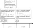
In this paper we reestablish, in a setup characterized by noisy signals on fundamentals, many of the “indeterminacy” results typical of the standard Obstfeld (1996)-type currency attack models. We use a simple two-period framework in which private agents not only need to choose whether to attack the peg or not, but also have to decide upon their future wage level. Therefore, wage-setters need to formulate expectations concerning the probability of the future devaluation. The subjective devaluation probabilities influence the inflation expectations, which, in turn, affect the following-period (average) wage level and hence unemployment. In this way, first-period expectations affect the second-period fundamental and thus the policymaker's future ability to resist an attack. We consider an extreme form of “decentralized” wage determination in order to stylize a situation in which the informational asymmetries among agents can play a role at the wage determination stage. We show by means of numerical simulations that, with realistic parameterizations of our economy, the equilibrium expectations may be either optimistic or pessimistic. Optimistic (pessimistic) expectations involve a second-period equilibrium characterized by a low (high) probability of devaluation, which then validates the expectations. We ascribe our results to the fact that agents decide upon the next-period wage having perceived whether the policymaker has resisted the current-period attack or not. This publicly available information reduces agents' uncertainty about the state of the economic system and about the other agents' perceptions, allowing for equilibrium multiplicity.
In our model, when the wage-setters are “optimistic,” and tend to coordinate with a low probability on the high wages equilibrium, the multiple equilibria region is larger than the one computed when they are “pessimistic” (and choose with a high probability a high wage). In the first case, the policy maker is more willing to resist a first-period attack because low wages imply a stronger second-period fundamental. Hence, the benefits of having kept the peg in the first period are higher. In this way, the coordinating device used by wage-setters influences the strategies adopted by the other players.
We also analyze an alternative setting in which wage-setters (imperfectly) observe the share of speculators who decide to attack the peg. This additional information raises the level for the fundamental involving a defense of the peg, while shifting upward the fundamental level compatible with a pessimistic equilibrium. These results bear interesting implications for a policymaker designing an (ex-ante) transparency policy: a transparent line of conduct is beneficial because it may prevent the possibility that agents coordinate on the “attack” equilibrium.
A small but growing literature has recently reconsidered the issue of equilibrium uniqueness in models of currency crisis grounded on private information.
Morris and Shin (1999), Rey (2001), and Metz (2002) emphasize that, in models in which agents receive a public signal in addition to their private ones, equilibria are multiple when the public signal is precise enough in comparison with private signals. When this is the case, the public signal's “coordination effect” becomes large and induces equilibrium multiplicity.2
Hellwig (2002) generalizes this result in a game-theoretical framework.
Although Tarashev's paper has the important merit of discussing the assets price informational role in the global games context, we provide a framework in which multiple equilibria can be obtained without introducing, as Tarashev does, the assumption that agents' demand incorporates the information provided by the current-period equilibrium interest rate. Also, in Tarashev (2001), equilibrium uniqueness is preserved when the stochastic disturbance to home asset supply is relatively large, a situation that may be considered “realistic.”
We assume, as do Morris and Shin (1999) and Metz (2002), that private signals are sufficiently precise to preserve equilibrium uniqueness during the currency attack.
Chan and Chiu (2002), in a static currency-crisis model, consider an exogenous (and publicly known) limitation for the support of the fundamental and verify that the equilibrium uniqueness result does not survive the introduction of this assumption. What is lacking in these situations is the presence of “extreme agents”—that is, of agents whose beliefs about the fundamental are so bad (good) that any other speculator is sure that they are (are not) going to attack the peg. The absence of such agents limits the uncertainty perceived by each speculator about other agents' beliefs, thereby making indeterminate the speculators' inference problem and hence restoring the multiplicity of equilibria. The results we obtain are deeply related to the ones achieved by Chan and Chiu. In fact, as already remarked, our agents decide upon the next-period wage having perceived whether the policymaker has resisted the currency attack. This publicly available information induces the agents to consider impossible a subset of the “states of the world.” This plays a role analogous to the one performed by the limitation on the support for the fundamental in Chan and Chiu. However, in our settings, such “limitation” arises endogenously, rather than exogenously, being conveyed by the rational exploitation of the information released by the currency attack itself.
According to Chamley (2003), the issue of the extension of the support can become decisive in a multiperiod setting. If, during any period, the speculators may restrict the support for the fundamental—for example, by exploiting their observations regarding other agents' actions—uniqueness is preserved only if, at the beginning of the following period, a new shock regenerates the original width for the fundamental's range. In our model, we will assume a stochastic structure that restores the original range for the fundamental at the beginning of each period.
Finally, in Angeletos et al. (2003), the central bank moves first by choosing the level of the interest rate, thereby providing a signal about its perception of the fundamental. Even if agents observe the fundamental with idiosyncratic noise, the informational content of the interest rate decision leads to a multiplicity of equilibria characterized by different policies and by different levels of speculator's “ferocity.” In contrast to this contribution, our policymaker's choice set is limited to the (ex-post) decision as to whether or not to abandon the peg, and this decision does not deliver any signal to individual speculators.
The organization of the paper is standard. Section 2 outlines the model and specifies the timing and the information available to agents, whereas Section 3 analyzes the second- (and final-) period equilibrium. Moving backward, we then focus on the behaviour of wage-setters and on the first- (and initial-) period currency attack equilibrium. In Section 5, we allow wage-setters to (imperfectly) observe the share of speculators who decide to attack the peg. Section 6 concludes.
AGENTS, INFORMATION SETS, AND TIMING OF DECISIONS
Structure of the Economy
We consider a two-period version of a standard model of monetary policy in a small, open economy of the type adopted, for example, by Obstfeld (1996, 1997), Jeanne (1997), and others. Our country is pegging its currency at a fixed rate against a foreign currency. We maintain that the purchasing power parity rule holds, so that, in the case of devaluation, the time t (for t=1, 2) depreciation rate is identical to inflation (πt). We also assume that the unemployment rate (ut) is described by
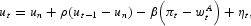
where un is the “natural” rate of unemployment4
The assumption of a constant natural rate is not essential, and it is introduced simply for expository purposes.
The persistence in unemployment embedded in equation (1) will play an important role in our model. In fact, it implies that the information about the period t realization of the disturbance is relevant in forecasting time t+1 unemployment. Hence, any asymmetry concerning the information about the period t fundamental implies the presence of heterogeneous forecasts for time t+1 unemployment.
Many theoretical and empirical papers provide support for the inclusion of some unemployment persistence in a macroeconomic model. Blanchard and Wolfers (2000) suggest that the high and persistent level of unemployment that characterized many European countries in the eighties and in the nineties can be at least partly explained by the interplay of shocks with rigid market institutions. Lindbeck and Snower, in their 2001 survey, point at labor turnover costs as the main determinant of employment (and hence unemployment) persistence both at the firm and at the aggregate level. Whereas the above explanations mainly focus on labor demand factors, Ljungqvist and Sargent (1998) study the effects of the welfare state on the supply of labor. In their model, unemployment benefits depend on the workers' past earnings and induce jobless workers, whose skills depreciate during the unemployment spell, to significantly reduce their search effort for new jobs. In this framework, transient shocks can easily generate persistent unemployment because jobless workers—whose ability is shrinking over time—have difficulty in finding jobs that they prefer to their unemployment compensation. At the empirical level, the structural VAR analysis conducted by Balmaseda et al. (2000) supports, for almost all the OECD countries, an identification scheme based on unemployment being persistent but stationary. More recently, Fève et al. (2003) estimate, again for the OECD countries, a model including equation (1) and find strong evidence of a persistence parameter that assumes values close (but not equal) to unity.
In our model, when the peg is defended, and hence inflation is set to zero, the unemployment rate—denoted by the superscript p—is as follows:

Agents
There are three types of agents: wage-setters, speculators, and a policymaker.
There are an infinite number of wage-setters, who are indexed by the superscript z and are referred to as if they were all female. As we specify below, wage-setters need to decide their period 2 wages at time 1. Wage bargaining is completely decentralized: each worker determines her own wage on the basis of her private information about the state of the economic system. In particular, each wage-setter chooses the growth rate for her nominal wage (w2z) by targeting her expectations about period 2 inflation,

where E[·] denotes the conditional expectation operator. The relevant information set will be specified below. What we have in mind is an economic system in which the workers are concerned about their wage purchasing power, which they want to preserve. Moreover, they are aware that—if the increase in their wage is below (above) the inflation rate—they will be forced to supply an excessive (too low) amount of working hours, because they are substitutes for firms, which retain the “right to manage.”
With no loss of generality, we assume that the total mass of wage-setters is one.
Speculators, indexed by the superscript i, are risk-neutral, their measure is h, and they are assumed to be male. Each investor holds liquid wealth (inclusive of his borrowing potential) equal to unity, and he decides in both time periods whether to speculate against the domestic currency or not. If he speculates, he buys the foreign currency on the forward market,5
Basically, we are assuming that the supply of foreign currency on the forward market is infinitely elastic. This modelling strategy implies the presence in the backstage of “uninformed” or “passive” agents who buy the currency from speculators. This is an (unpleasant) feature that we share with the existing literature (see Morris and Shin, 1998, 1999; Chan and Chiu, 2002; Metz, 2002; and Heinemann and Illing, 2002). Tarashev (2001) provides a more sophisticated way of modelling demand and supply functions, which could be embedded in our framework. However, this would obfuscate our result because a second source of multiplicity would be added to the model.
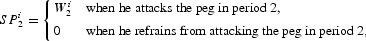
where W2i is the expected profit yielded in period 2 by speculation, conditional on the time 2 information set; the payoff of not attacking is normalized to zero. The speculator's payoff in period 1 is

where W1i is the expected profit yielded at time 1 by speculation, conditional on that time information, whereas p1i is the subjective probability that the speculative attack is successful and the peg is abandoned in period 1. The discount factor, which plays no substantial role in our model, is unity.
Provided that the peg has not been abandoned in the past, the domestic policymaker decides, in each period, whether or not to abandon the peg in order to minimize her or his intertemporal loss function,

where Lt(·) is the period t loss. We assume that when the policymaker decides to abandon the peg, the devaluation is of the fixed size
.6
Although it would be possible to defend such an assumption (
could, for example, be the devaluation needed to obtain the current account equilibrium), we admit that this hypothesis has been introduced because it significantly reduces the computation time for the numerical solution of our model. In the working paper version of this work, we allowed the policymaker to determine the optimal πt, but at the price of considering single-period loss functions. We deemed this price to be too high.
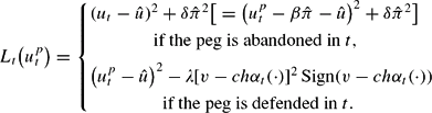
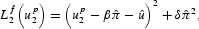
The first line is a standard quadratic loss function that applies when the peg is abandoned:
is the optimal unemployment level for the policymaker, and δ>0 is a parameter capturing the policymaker's “aversion” to inflation. This quadratic loss function applies also when the peg has been abandoned in a previous period. In this case, the time t inflation rate,
, is incorporated into the average wage and thus—via equation (1)—influences the period t unemployment.
The second line becomes relevant when the policymaker defends the peg. Its second addendum reflects the additional costs and benefits generated by keeping the peg. The benefit, v, is expressed as a share of GDP. This benefit captures a number of factors, such as increased investment and foreign trade generated by the reduction in exchange rate uncertainty or the political and economic advantages arising from the possibility of joining a monetary union (as might be the case for some central European countries).7
The establishment of anti-inflation credibility also plays a role, which should be modeled explicitly.
Although the availability of reserves need not be an issue of paramount concern for a government or a central bank that has access to the world capital market (as emphasized, for example, by Obstfeld, 1994), borrowing foreign currency on the market is expensive (and may involve political costs).
The net benefit of the defence is weighted by λ>1.
We now introduce the following:
Assumption 1. v<ch.
Assumption 1 implies that for sufficiently high values of αt(·) the cost of the defense of the peg outweighs the per-period benefits (equation (3)). Hence, we shall consider both the case of a positive per-period benefit and the case of a negative one, making the discussion more general.
Timing of Events and Informational Structure
Every agent enters the first period having observed the past realizations of all the relevant variables. In line with the existing literature, we assume that he or she also knows the natural unemployment rate, the policymaker's preferences, the parameters characterizing eq. (1), and the structure of the stochastic disturbances. This knowledge is taken as understood: hence, we denote the time 1 common information set by
.
At the beginning of time 1, both speculators and wage-setters receive signals, denoted by s1i and s1z, respectively, concerning the shock currently affecting the economic system. (More details about the structure of the signal will be provided shortly.) At this stage, speculators—whose private information set is
—decide whether to attack the peg, and the policymaker decides whether to resist or to devalue. Having observed whether the peg has been abandoned or not, the workers fix their next-period wage, contracting for it directly with their employers. Notice that the wage-setters' information set is
.
At this point, two comments are in order. First, we consider a “decentralized” bargaining environment because even the most casual observation suggests that agents' forecasts are different; thus, we found it of interest to analyze a framework in which agents' actions are driven by their diversified beliefs. Notice, moreover, that the polar case, based on the assumption of a single union determining wages, is equivalent to the hypothesis of common information at the wage-setting stage. Not surprisingly, such an assumption easily leads to multiple equilibria (as shown in the working paper version of this contribution) because it eradicates any coordination problem from the wage decision taken during period 1 and affecting period 2.9
Both the assumption of completely decentralized wage bargaining and that one of a single union may seem extreme. Admittedly, they represent useful starting points because they simplify the analysis. However, we have verified by means of numerical techniques that, as intuition suggests, when the number of unions contracting wages is finite, equilibria are multiple if they are so for an infinite number of wage-setters.
Second, as already remarked, at the wage-setting stage any private information set incorporates the knowledge about the effectiveness of the defence of the peg. Hence, the one-period-ahead wage is decided upon by exploiting the informational content of the observation concerning the successfulness of the currency attack, a fact that is of remarkable importance in what follows. However, we assume that each agent must conclude her wage contract without knowing the wage agreed upon by other agents. If these data were available, each individual worker could extract information about the signals received by the others: this scenario would become more similar to a “centralized” wage-bargaining scenario (and the model would become analytically intractable).
In period 2, the realization of the time 1 disturbance and of the time 1 (average) contracted wage become common knowledge, so that
. Investors receive a signal about the time 2 disturbance (hence,
and decide again whether to attack the currency in the light of the new information; the policymaker decides whether to resist the attack or not. (Figure 1 summarizes the timing of events).

The timing of events.
The signal received by an agent on any particular date is private and potentially different from the signals received by others. The signal received by each agent—who knows only imperfectly the fundamental—concerns the realization of the stochastic disturbance ηt. To save on notation, we assume that the signals received by speculators and wage-setters are characterized by the same structure and by the same parameter values. Focusing, to save space, only on speculators, we specify the signal as
, where εti is a normal random variable with zero conditional mean and variance σε. We assume that every εti is independent from ηt and over time (these hypotheses can be relaxed).
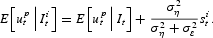
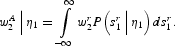
Notice that receiving a signal about the disturbance is equivalent to obtaining a signal about the level of unemployment that would prevail in the economy when the peg is defended. The normality of the disturbances εti, in conjunction with the normality of ηt, allows the exploitation of the Bayesian learning model to obtain
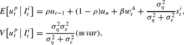
where
denotes the variance of
conditional on the information set
.
These expressions summarize the belief each agent i develops about the realization of the fundamental at the beginning of time t. When calculating
, the weight attributed to the private signal is positively linked to its precision and to the variance of the disturbances. Notice that the conditional expectation for the fundamental can be expressed as
We assume, following the existing literature, that the policymaker perfectly knows the state of the economy and hence the realization for ηt;10
Alternatively, one could build the model specifying that what matters in (3) is the policymaker's perception of unemployment.
which sum up the knowledge the policymaker has about individuals' signals.
SECOND-PERIOD EQUILIBRIUM
We start by analyzing the period 2 equilibrium, and we then move backward to period 1. In what follows, we first clarify the government's optimal policy, we then describe the speculators' behavior, and finally we characterize the second-period equilibrium.
Policy Analysis
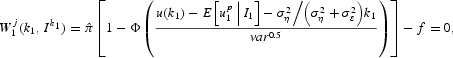
When the policymaker opts to leave the peg, its loss (
is
while, if the fixed exchange rate is maintained, its loss becomes

For any given
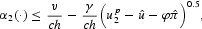
(and hence for any given η2), the policymaker's optimal decision is to defend the peg if
, an inequality that boils down to

Assume that
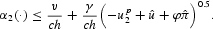
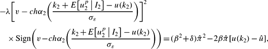
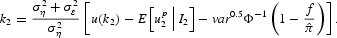
, where φ=(β2+δ)/2β. In this case, the left-hand side of the inequality above is negative. Thus, inequality (6) can be fulfilled only if Sign(v−chα2(·)) is positive and therefore α2(·)<v/ch. In this case, the above inequality is satisfied—and hence the peg is defended—when
where
. The obvious restriction α2(·) ≥ 0 implies
. When
, the policymaker opts out of the fixed exchange regime even if nobody speculates against the currency.
Now consider the case
, so that the left-hand side of inequality (6) is nonnegative. In this case, (6) not only is satisfied when α2(·)<v/ch but also can be fulfilled if α2(·)≥v/ch. When α2(·)≥v/ch, the defense of the peg requires the following further restriction:
Because α2(·)≤1,
; when
the peg is defended even if every agent attacks.
Notice that equation (6) generates the tripartite classification for the fundamental that characterizes a large part of the literature.
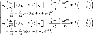
The Share of Attackers
Morris and Shin analyzed in various contexts (e.g., 1998, 1999) the optimal behaviour of risk-neutral attackers in a global game framework. They propose a monotone-strategies equilibrium, where two key elements characterize the speculators' optimal behavior: all the agents who obtain a signal larger than a trigger k2 attack the currency, whereas no speculator observing a signal lower than the trigger participates in the attack.
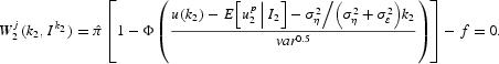
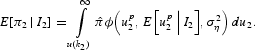
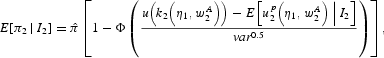
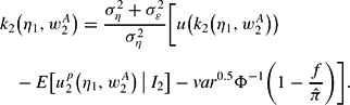
The policymaker is aware of this behavior, and so—given k2—he or she exploits his knowledge about the individuals' signals [equation (5)] to compute the share of attackers for any given realization for η2 (i.e., for any given level for the fundamental),
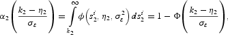
where ϕ(a, b, c) is the probability density function at a for a normal random variable with conditional mean b and conditional variance c; Φ(a) is the value of the cumulative density function for a standard normal computed at a. We will denote by ϕ(a) the probability density function at a for a standard normal distribution.
We now prove
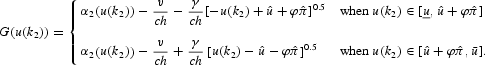
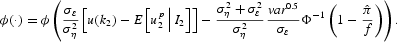
PROPOSITION 1. For any given k2, a unique threshold u(k2) exists, such that the policymaker decides to opt out of the peg for u
and to defend the peg otherwise.
Proof. Refer to Appendix A.
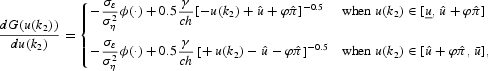
Figure 2 shows how the share of attackers (equation 8) and the resistance curve (given by equations (7a) and (7b)) determine the resistance threshold u(k2) as a function of the trigger signal k2.

Determination of the resistance threshold u(k2).
The fact that u(k2) can be uniquely determined as a function of k2 helps to build some intuition for the equilibrium we are considering. In fact, because any speculator can figure out the threshold level u(k2), he can compute his subjective probability that the peg is abandoned (which is, the probability that
). Because a speculator makes money only when the attack succeeds, his expected utility depends positively upon his assessment about the probability of a successful speculative episode, which is increasing in the speculator's private signal. Hence, the expected profit for any speculator is increasing in the signal he receives. Therefore, when an agent observing
finds it profitable to attack, he can be sure that all the speculators with larger signals will do the same. Similarly, when an agent receiving the signal
prefers not to attack, he can be sure that all the speculators observing a smaller signal will refrain from attacking.
Attackers' Payoffs
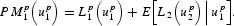
The expected profit for an attacker is given by the expected capital gain minus the cost that he must incur when speculating; in turn, the expected capital gain is given by inflation (
) multiplied by the subjective probability of a successful attack (which is the expression in the big square brackets is the equation below).
When speculators follow the equilibrium strategies we have described in the previous section, the expected profit for an agent i who decides to participate in the speculative attack—believing that the currency is attacked only by the agents who receive a signal larger than the threshold k2—depends on his own signal and on the resistance threshold, which in its turn depends on k2.
Hence, the period 2 expected profit for an attacker is
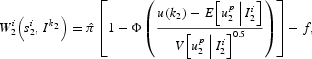
where Ik2 is a function indicating that—at time 2—the attack is run by all the agents observing a signal larger than or equal to k2 (and only by them) and f is the cost that one must incur when speculating against a currency. Exploiting equation (4), we manipulate the above expression to write
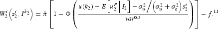
Some algebra allows verification that ∂W
(s
, I
/∂s
is positive, as intuition suggests.
Second-Period Currency Attack
We now analyze the equilibrium outcome of the speculative attack taking place in period 2. Because we need to determine simultaneously the resistance threshold u(k2) and the trigger signal k2, we need two equilibrium relations. The first one is equation (6), in which the share of attackers is given by (8),
where, for convenience, we have exploited the fact that
.
The second equation simply states that the “marginal speculator” (i.e., the one receiving the lowest signal allowing for participation in the attack (k2)) makes zero expected profits:
Adapting the argument provided in Morris and Shin (1999) and Metz (2002), we now prove
PROPOSITION 2. If
, the period 2 equilibrium is unique.
Proof. Refer to Appendix A.
Thus, to guarantee the uniqueness of the “currency attack” equilibrium, we introduce the following:

So far, we have simply confirmed Morris and Shin's main result: provided that the variance of the private signals is sufficiently small in comparison to the variance of the true process, there is a unique period 2 equilibrium. It is the presence of agents receiving very high (larger than
or very low (smaller than
signals that induces the uniqueness of the equilibrium. In fact, for a speculator obtaining a very high (low) signal, it is a dominant strategy (not) to attack the peg, because he believes that the peg is (not) abandoned even if nobody (everybody) attacks. The knowledge that agents with “extreme” beliefs have a dominant strategy makes the same strategy dominant also for the speculators receiving “almost extreme” signals, because they are “almost sure” that a sufficient share of speculators will (not) attack the peg. Iterating this reasoning leads speculators to select the strategy prescribing to attack only upon receiving a signal larger than k2.
The fact that equilibrium uniqueness is granted only if private signals are sufficiently precise can be understood by considering that the period 1 realization for the fundamental—being known by everybody at time 2—plays the role of a public signal. Therefore, it helps any speculator to make some inference about other speculators' beliefs, and therefore about their actions. If the public information is sufficiently precise relative to private signals, its coordinating effect becomes so large that it induces multiple equilibria.
However, the uniqueness result holds conditionally on the wage, which was determined during period 1 and—up to now—taken as given. Hence, to fully characterize the equilibrium, we need to connect the determination of the wage rate with the outcome of the currency attack.
Before we undertake this task, notice that the observation of the period 2 currency attack equilibrium implies the obtaining of some information about the realization of the stochastic disturbance η2. When the attack fails, every agent understands that
, which means that
; moreover, notice that such information is common knowledge. As we shall argue below, the information revealed by the currency attack plays an important role.
Finally, notice that the two thresholds characterizing the equilibrium, k2 and u(k2), are computed without referring to any particular information set. Private signals, in addition to providing the rational basis for the adoption of monotone strategies, determine the identities of the attackers.
FIRST-PERIOD EQUILIBRIA
The purpose of the next two subsections is to show that, even when Assumption 2 is satisfied, the equilibrium uniqueness does not survive to the endogenous determination of inflation expectation and wages. Working backward, we first determine the average wage contracted during period 1 for period 2, conditional upon the survival of the peg, and then analyze the first-period currency attack (see Figure 1).
Wage Determination
As already mentioned, we assume that every wage-setter contracts her own wage on the basis of her private information about the state of the economy because this is a simple way to allow for an active role of time 1 informational differences. Notice that wage-setters know whether the peg has been abandoned or not; we focus our attention on the case where the peg has been defended and wage-setters are aware that, as suggested by our previous analysis,
, where
is determined during the currency attack phase and it is—for now—taken as given.
Because every wage-setter picks her wage by targeting her expectations about period 2 inflation (equation (2)), the wage she chooses in period 1 is

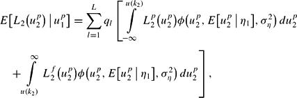
The determination of the time 2 individual wage for agent z is not trivial because, from the perspective of the first period, her time 2 expected inflation depends upon the average wage, which in turn is determined by the integral sum of individual wages. In addition, the average wage influences unemployment, via equation (1), and hence the likelihood of a successful period 2 defence, which in turn affects expected inflation.
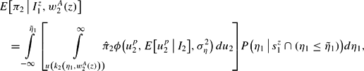
We analyze the formation of individual inflation expectations in three steps. First, we investigate the inflation expectation, as it would be determined at the beginning of the second period on the basis of the common information set I2 (which includes wA2). We then use this result to show how the wage-setters' subjective period 1 inflation expectations are formed, given the average wage. Finally, we determine the average wage.
At the beginning of the second period, wage-setters know the realization for η1 and the average wage contracted during period 1, w2A. Hence, the expected inflation is
Solving the integral, we write
where we highlight the dependence of the fundamental
and of the resistance threshold
on the realized values for η1 and
.
At time 2, any wage-setter can compute the threshold
as part of the unique solution for the system:

In period 1, each wage-setter—for any given average wage—can compute the one-period-ahead inflation expectation conditional upon her imperfect information about η1. What any wage-setter does for a given average wage is to weight the inflation expectations conditional on η1 by her subjective realization probabilities for η1,
where
is the probability that agent z, receiving signal
and observing that
, assigns to the event that the true realization for the process affecting the fundamental is η1.12
Some details about
are provided in Appendix B.
: what a wage-setter actually knows is her subjective estimate for the average wage. For a given
, the individual wage [equation (11)] becomes
At this stage, we must take into account the fact that any wage-setter z is aware that the other agents receive different signals and, hence, that using their information sets, they compute different wages. Any agent z can calculate, from the standpoint of her information set, the average wage,
where
is the probability that agent r receives signal
given that agent z has received signal
and that
.13
For details about
refer again to Appendix B.
We define as a wage-setting equilibrium a situation in which (a) every wage-setter z computes her subjective inflation expectations, using equation (14), on the basis of the average wage w2A(z) obtained from equation (14), and (b) every private wage increase, being determined through equation (13), is consistent with the subjective inflation expectation and average wage.
Notice that the wage-setting equilibrium is conditional upon the true state of the economy (which affects the private signals) and upon the first-period resistance trigger,
, which, as we shall discuss in what follows, can be seen as the difference between the first-period resistance trigger, u(k1), and the first-period expectation about the fundamental,
.
Finally, notice that with knowledge of the realization for η1 the policymaker can compute the average wage as determined on the market:
First-Period Currency Attack
In the first period, speculators must decide whether to attack the peg, whereas the policymaker chooses whether to resist on the basis of his or her intertemporal loss function. As we did for the second period, we need to determine a trigger signal (which determines the speculators' behavior) and a resistance threshold for the policymaker. Notice that the policymaker's decision depends on his or her computations about
, because the second-period average wage affects his or her second-period loss.
Now, we encompass the possibility that there are multiple equilibrium distributions for wages. Following a relevant portion of the literature, we assume that, when equilibria are multiple, wage-setters coordinate using a “sunspot” variable. We denote by L the number of equilibria and by ql the probability that wage-setters coordinate on a specific equilibrium (that is, that the sunspot variable takes the values related to a specific equilibrium). Obviously,
Now, notice that the speculators' first-period behavior can be characterized in the same way that we portrayed their time 2 conduct. In fact, because speculators are atomistic, they do not take into account the (actually negligible) impact of their first-period action on the probability of survival for the peg. Hence, their continuation value,
, is independent of their first-period decision with regard to the position they take. Because the continuation value is identical whatever action they take, speculators only care about their first-period expected payoff.
Thus, all those who receive a signal higher than the one obtained by the marginal speculator attack the peg:
where u(k1) is the peg abandonment threshold for the policymaker.
When the policymaker decides to defend the peg against the first-period attack, he or she obtains in that period the following loss:

Defending the peg, the policymaker grants himself or herself the possibility of opting out of the fixed-exchange-rate regime during the second period. Because the policymaker can compute the average wage(s) that is (are) going to be established on the labour market given up1 (which implies the knowledge of η1), the expected time 2 loss is
where, to save on notation, the dependence of
and of u(k2) on the average wage,
, and hence on the realization for the sunspot variable, is taken as understood.
Accordingly, the total loss involved by keeping the peg during the first period is
When the policymaker decides to float the currency at time 1 he or she obtains the following first-period loss:
The second-period expected loss is computed taking into account the fact that the second-period wages will be set equal to the second-period inflation,
:
As before, the total loss involved when the peg is abandoned during the first period is given by the sum of the losses in the two periods:

Because the peg is defended at time 1 whenever
, the resistance threshold is defined by the equality
which is the intertemporal counterpart of equation (9).
Numerical Results
The system composed of equations (9), (10), and (12) to (17) determines k1, k2, the resistance triggers u(k1) and u(k2), the individual wages
, the subjectively computed average wage
, the inflation expectations, and the true average wage
. This system cannot be solved analytically, and thus we need to rely on numerical techniques.14
Our routine, written in Gauss, relies on several simplifications. In particular, we have discretized the support for the signal
, and we have considered a set of 1001 agents receiving signals distributed in the range [−0.01, 0.19]. In addition, we have truncated any normal random variables, considering the support [μ − 6σ, μ + 6 σ], where μ and σ are the mean and standard deviation for the variable. We have provided each agent with an initial guess for the aggregate wage, and we have let the routine calculate a vector of aggregate wages (
, which has been used iteratively as a set of initial guesses. We considered that the routine successfully converged when the sum across agents of the difference (in absolute value) between the initial guess and the computed
was lower than 10−8. We regard the relatively small number of agents as the main limitation of our numerical exercises; however, we decided to restrict our experiment to that number because our routine takes about 3 hours to converge on a Pentium IV/2400 personal computer. Also, when we increased the number of agents from 601 to 1001 our results were not significantly affected.
We now provide numerical values for the parameters (β, δ, λ, ρ, f, σε, and ση). In addition, we offer a quantitative assessment of the benefit obtained by maintaining the exchange rate (v) for the cost of the defence against speculation (determined by the product of c by h), for the natural rate, un, for the target level of unemployment,
, and for the inflation rate prevailing in case of free floating,
. A probability distribution for the sunspot variable must also be provided. Because in all of our calculations we have been able to identify at most two equilibria, what is actually needed is a value for the probability q of an equilibrium where wages are high (i.e., of a “pessimistic equilibrium”).
For some of our parameters a convincing value is easily provided. Some empirical studies suggest that, in the United States, the sensitivity of unemployment to wage growth and inflation is high; accordingly, the most frequently used value for β is one, when the calibration is based on annual data. We fix β to 0.5 to accommodate the fact that the relationship between inflation and unemployment seems to be looser in many countries—such as those in the Euro area—than in the United States. The standard deviation ση has been assigned the value 0.01, which implies that in two cases out of three, absent monetary policy surprises, the annual change in the unemployment rate is below 1%. The speculation cost f has been set to 0.03 to take account of transaction costs and of a small differential between the domestic interest rate and the “world” one.15
Reasonable perturbations of this value do not significantly affect our result.
The parameter summarizing the policymaker aversion to inflation is clearly a more difficult choice. We opted to fix δ=0.5, which implies a policymaker rather averse to accommodation (compared with the one in the exercises proposed by Obstfeld, 1997).
We chose λ equal to 3, attributing a relatively high weight to the net benefits obtained by defending the peg, and ρ=0.9, which is in line with many empirical estimates. As we shall comment below, a high ρ tends to shrink the “multiple equilibria” area.
Further problems are posed by
, v, c, and h. Here we assume that
% because this value corresponds to the inflation rate that is optimal for a policymaker characterized by the proposed loss function, when unemployment is in the middle of the interval
. Then we take a shortcut: we assume that v=0.03 and ch =0.08 because this choice implies that
and
.16
Notice that ch = 0.08 implies a ratio equal to 2 between the “hot money” that can potentially attack the country and its GDP when the financing cost is 0.04%.
, we obtain reasonable dimensions for the region in which the country is “ripe for attack”; we also set
.17
The “target unemployment” usually plays an important role in currency attacks models because the difference un–
may be considered an indicator for the extent of the time inconsistency problem affecting the policymaker. However, different choices for
and un would only shift the “attack region” (and the “multiple equilibria region”); because we do not tackle the important issues involved by the ex-ante policy evaluation, these effects are not significant.
We now choose q=0.5, we add σε=0.10% to the constellation of values described above, and we assume that the time 1 disturbance, η1, takes its most likely value (zero) (hence u1=E[u1[mid ]I1]). Having provided a baseline value for every parameter, we set to zero the first-period average wage (w1A) and we obtain model simulations conditioned on the initial unemployment value. The first column in Table 1 shows the initial condition, ranging from 7% to 9%; the second highlights the policy maker's strategy, providing the unemployment threshold,
. Notice that the peg is defended in all the cases we have considered except for u1=9%, where u(k1)<u1. The third column describes the trigger signal characterizing the speculators' behavior (u′1). This has been reported in terms of the fundamental—instead of the disturbance η1—to help the reader's intuition (bear in mind that u′1≡k1(u1)+u1). The fourth column shows the first-period share of attackers implied by u′1, which is α1((u′1−u1)/σε)≡α1(k1(u1)/σε), because η1 = 0. As the fundamental increases, the attack trigger diminishes and the share of attackers increases, because the speculators—perceiving that the abandonment is more likely—are more inclined to attack. The fifth and sixth columns are crucial: they show the policymaker's computations of the two possible average wages, as determined on the market. The actual realization for
causes the economic system to move to the second or to the third section of Table 1.

The first column in the second section of Table 1 shows the second-period expected unemployment, determined by equation (1), when the average wage is low. The resistance threshold u(k2) is presented in the second column, whereas the third shows the second-period trigger signal. These are both decreasing in the second-period unemployment, because a weaker fundamental reduces the resistance payoffs and makes the speculators more willing to attack, because they (subjectively) perceive that the abandonment probability increases. Column four provides the time 1 expected share of second-period attackers, which increases as the trigger signal decreases. The last column in the second section of Table 1 shows the expected probability of a second-period default, as computed by the government at time 1. The fact that the second-period resistance threshold and trigger signal are much higher than those characterizing the first period is due to the fact that an early abandonment of the peg is more appealing for the policy maker, because the reduction in unemployment it conveys exerts positive effects on the second period. The last line describes what happens when u1=9% and hence the peg is abandoned at time 1. In this case, the surprise inflation reduces unemployment in period 1 (by
; because the first-period unemployment drops to 4%, which is the “natural level,” its expected value for the second period does not move (refer again to equation (1)).
The third section of Table 1 shows what happens when the wage-setters select—during the first period—the “pessimistic equilibrium.” In this case, when the peg survives the attack at the beginning of time 1, the expected second-period fundamental is higher due to the negative effect of higher wages on employment. Accordingly, the resistance threshold for the policymaker and the trigger signal for speculators are lower, whereas the expected share of attackers and the expected probability of default are higher.
Having established that multiple equilibria can emerge, we characterize the “indeterminacy area” for σε∈{0.05%, 0.10%, 0.15%, 0.20%}, considering three alternatives for the probability of a pessimistic equilibrium at the wage-setting stage. In the first scenario, wage-setters are (and are known to be) “optimistic,” so that q=0.1; in the intermediate case q=0.5; in the third one pessimism prevails (q=0.9). As before, we consider the case η1=0; we define as “multiple equilibria” a situation in which our routine—starting from different initial conditions—computes two equilibrium average wages the difference of which is larger than or equal to one percentage point.
The “multiple equilibria” range is summarized in Table 2, where we denote by
and by
, respectively, the lowest and the highest value for unemployment such that our routine computes two equilibria.

When
, the peg is maintained in period 1, and the equilibrium wage distribution is unique, being characterized by wages low enough to guarantee probabilities of a successful second-period defence close to unity.
For
, the policymaker keeps the peg, but there are two equilibrium wage distributions, implying respectively high and low probabilities of a time 2 defence of the peg.
Finally, when
, the peg is abandoned in the first period.
Table 2 provides also the “trigger signals” that correspond to
and
, that is,
and
, therefore characterizing the speculators' behavior. Not surprisingly, as the threshold decreases, the corresponding trigger signal gets larger, because the speculators—perceiving that the fundamental is sounder–are less inclined to attack.
Several remarks are in order. First, the range for the fundamental for which we have found multiple equilibria is relevant, going from 1.26% to 2.33%.
Second, the comparison of the results obtained for q=0.1 and for q=0.9 shows that, when the wage-setters coordinate with a low probability on the “high-wages” equilibrium, the threshold
is higher than in case of a high probability for the pessimistic outcome. The intuition for this result is clear: the policy maker is more willing to resist a first-period attack when she or he knows that the probability of a second-period low-wages equilibrium is high. In fact, when wages are low, the second-period currency attack is characterized by a lower share of attackers because—ceteris paribus—the fundamental is stronger; hence, the benefit of having kept the peg in the first period is higher. The policymaker's willingness to resist also influences the first-period behavior of the speculators, who become less inclined to attack. Therefore, in the case under scrutiny, the coordinating device used by the wage-setters influences the strategies adopted by the other players during the first-period attack, so that
, and hence the resistance areas are significantly affected.
It may be surprising to notice that the results for q = 0.1 and for q = 0.5 are identical. This is due to the fact that, for q = 0.5, the benefits obtained by the policy maker thanks to the first-period defence are already high enough to imply resistance for any u1 such that the “low-wages” equilibrium exists. Hence, a reduction in q is ineffective in increasing the resistance area: for the policy maker it is pointless to enhance her or his resistance threshold. In fact, to defend the peg with a higher fundamental is tantamount to resisting in a situation where the low-wage equilibrium does not exist. This policy cannot be optimal because a high-wage growth implies an almost sure abandonment of the peg in the second period, undermining the advantages of a first-period resistance.18
A lower value for λ—which is for the weight attributed to the benefits obtained by the government defending the peg (net of the cost of the intervention)—reduces the range for q so that the resistance area does not change.
Third, we notice that—in most cases—the upper bound for the interval (
is increasing with the standard deviation for the private signal. This contrasts with the effect emphasized by Metz (2002). In her paper, when—as is the case—the fundamental is perceived ex ante as unsound, an increase in the variance for private signals tends to make speculators more aggressive. In fact, if private signals get less precise, speculators tend to give more prominence to the public information (that is, to the ex ante expected value for the fundamental), which tells them that the fundamental situation is gloomy. Hence, for a given expected fundamental, the unemployment rate and the signal trigger get lower. In our model, when u1 is close to
, information is relatively homogeneous among wage-setters; thus, they can coordinate on low wages. To appreciate this point, consider the case in which
. When those agents who have been induced by their signal to believe that
observe that the peg has survived, they must significantly revise downward their belief about u1. Hence, wage-setters' information becomes more homogeneous, allowing coordination on the “low-wage” equilibrium, which enhances the benefits of keeping the peg and therefore raises the defense trigger. This effect is more important the larger the standard deviation for private signals: the higher the signals' precision, the lower is the effect of further information. In most cases, this positive relationship between the standard deviation and the resistance trigger outweighs the negative effect highlighted by Metz, hence the link between the upper bound of the multiple equilibria interval and the variance for private signals is positive.
Fourth, the lower bound for the multiple equilibria interval (
is mildly decreasing with σε. An increase in the variance in private signals implies that a greater proportion of agents receive a high signal. This tends to make it easier to coordinate on a pessimistic equilibrium, which increases the “multiple equilibria” range, reducing
.19
Notice that this result partly contrasts with those obtained in a very different context by Herrendorf et al. (2000), where the heterogeneity among agents tends to reduce the scope for multiple equilibria.
Notice that the reduction in the pessimistic expectation area does not necessarily imply that the policymakers should try ex ante (i.e., before observing u1) to let individual agents receive precise signals (i.e., that a transparent policy should be pursued). In fact, a decrease in σε, although reducing the area where the economic system finds itself in the multiple equlibria region, increases the area where the peg is abandoned in period 1.
We have found that the error autocorrelation parameter, ρ, is relevant in determining the interval where multiple equilibria are possible, as documented in Table 3. More specifically, the lower is ρ, the wider that interval. The intuition for this result is simple: when ρ is low, the policymaker is aware that unemployment, ceteris paribus, is going to decrease more quickly in the future (equation (1)). Hence, he or she is more willing to resist the attack and keep the peg during the first period. This remarkably increases the upper bound for the “multiple equilibria” region,
.

To verify that the information released by the failure of the period 1 currency attack actually plays a crucial role, we have modified our routines to check what happens when wage-setters disregard this piece of information. We have found that, in this case, the multiplicity in the equilibrium wage distributions never arises. In this case, in fact, every wage-setter thinks that there are some agents obtaining an extremely high (low) signal on u1; these wage-setters are thought to fix a percentage wage increase equal to
(to 0). The wage setters receiving an in-between signal determine their average wage, taking into account the existence of all the other agents and hence also of those asking for a wage increase as high as
(as low as 0). This ties both the ends of the wage distribution, which turns out to be unique. In contrast, when agents exploit the information that
, there are no agents that consider sure an inflation rate as high as
and one end of the wage distribution is “loose.” Intuitively, when the agents receiving a signal slightly lower than
are pessimistic, they coordinate around a high-wage equilibrium, which can prove consistent with the fundamental and with the other agents' expectations. If, on the contrary, these wage setters are optimistic, they choose low wages, which are as well part of an equilibrium.
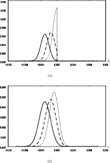
The “narrowing down” of the subjective distributions for η1 characterizing the agents who receive a signal close to
is portrayed in Figure 3a. There, the probability distribution
is drawn for three different signals, the difference between the lowest one (continuous line) and the intermediate one (dashed line)—0.0015—being the same as that between the intermediate and the highest one (dotted line). Figure 3b depicts the probability distributions
, given the values for
used to draw Figure 3a. Again, the presence of the threshold
induces the agents receiving high signals to tighten the distributions for the other agents' signals. These effects induce wage-setters receiving high signals to compute “relatively homogeneous”
.

(a) Probability distribution functions $P(\eta _1\,|\,{s_1^{z} \cap (\eta _1 \le \tilde {\eta} _1 = 0))}$ for $s_1^{z} = \{-0.0030, - 0.0015,0\}$. (b) Corresponding probability distribution functions $P(s_1^{r}\,|\,{s_1^{z}\; \cap}$ ${(\eta _1 \le\tilde {\eta} _1 = 0))}$.
Hence, the informational content of
makes agents, and especially agents receiving high signals, less uncertain about the fundamental and about the other agents' perceptions. Moreover, as already remarked, every agent knows that the fundamental is not in the “opt out” region. Therefore, they can coordinate their expectations.
INFORMATION DISCLOSURE DURING THE “CRISIS”
Up to now, we have assumed that the successful defense against the speculative attack involves the disclosure of a minimal amount of information: agents just perceive that unemployment is below the level involving speculators' success. However, an attack may reveal further information to any private agent. If agents observe the position taken by the speculators or—to consider a more realistic situation—if data about the reduction in official reserves are promptly made public, the agents obtain relevant additional information. In what follows, we assume that agents receive an additional private signal, which is, again, affected by an idiosyncratic shock. Hence, agents interpret these data in (slightly) different ways—an implication that we find realistic.
We assume that the new information concerning the ferocity of the attack is boiled down by any wage-setter z to a signal about the current-period disturbance taking the form

where v1z is a normal random variable with zero conditional mean and variance σv. We assume for simplicity that every v1z is independent from η1, from
, and over time. Thus, at the period 1 wage determination stage, any private information set is
. The normality assumption enables us to aggregate the two idiosyncratic signals,
and
, into a single composite signal,
which is normally distributed with
and
. Obviously, the composite signal is always more precise than the original one.
By adding the value σv=0.001 to the parameter set described in the previous section and by properly modifying our numerical routine we obtained the “indeterminacy area” that is presented in Table 4.

Comparing Table 4 with Table 2, we notice that, when σε>0.1%, the upper bound for the interval (
is (slightly) increased. To understand this point, bear in mind that the additional signal
is perceived by the wage-setters only. Hence, speculators' behavior is unaffected whereas wage-setters, when u1 is high, find it easier to coordinate on low wages, because their information is more homogeneous. This enhances the benefits of keeping the peg and therefore raises the defense trigger. This effect becomes quantitatively significant only when σε is relatively large: in this case, in fact, the presence of an additional signal has an important impact on
. The lower bound for the multiple equilibria interval (
is (again, moderately) increased by the presence of an additional signal. As we noticed in the previous section, a reduction in the variance for private signals makes coordination on the high-wages equilibrium more difficult for those agents who receive a low signal because their information is more homogeneous.
Notice that a transparent policy is always beneficial, because it increases the peg abandonment trigger
while shifting upward the multiple equilibria area (
.
CONCLUDING REMARKS
We have considered a currency crisis model in which agents' expectations influence the policymaker's future ability to resist an attack. In our framework, as in several Obstfeld-type models, the link connecting the future fundamental with current expectations is provided by the wage determination mechanism.
In the presence of heterogeneity in inflation forecasts, we find, for a relevant range in the initial level of unemployment, that equilibrium expectations are multiple. Optimistic (pessimistic) expectations involve a second-period equilibrium characterized by a low (high) probability of devaluation, which in turn validates the expectations. Moreover, because the benefits of keeping the peg in the first period are higher when the wage-setters are optimistic rather than pessimistic, the coordinating device used by wage-setters influences the policy maker's strategies (and hence also the speculators' behavior and the equilibrium multiplicity region).
A line of reasoning similar to the one developed in our paper could be applied in situations in which the role of the fundamental is played by external debt, as in Velasco (1996), and the policymaker may decide to devalue when interest payments become too burdensome. In general, the possibility of self-fulfilling sovereign debt crises, originally highlighted by Calvo (1988), could be reestablished.
Our analysis can be extended in various directions.
The period 2 information set contains the time 1 determined average wage (w2A). This can be viewed as the (publicly known) expected devaluation rate, which may well influence the short-term nominal interest rate. Hence, it would be sensible to investigate the consequences of the introduction of an “expected inflation” term into the period 2 cost of buying the foreign currency on the forward market. To take this possibility into account, we have run a modified version of our routine, finding that our multiplicity result is unaffected.
Building on Dasgupta (2002) and on Corsetti et al. (2004), one can analyze a situation in which imperfectly informed investors may decide to delay (within the same period) taking a position against the currency in order to (imperfectly) observe the other speculators' behavior and to refine their belief based on this observation. In this setting, if wages are set once the policymaker has decided whether to abandon the peg or not, our results are confirmed: the observation of the outcome of the attack provides a public signal, which induces the possibility of multiple equilibria.
In conclusion, our numerical exercises are effective in showing that in a model in which expectations affect future fundamentals and hence the policymaker's future willingness to resist to an attack, the problem posed by the “multiple equilibria” approach—both as a basis for forecasting and as a framework within which to ground policy analysis—cannot be solved by the presence of asymmetric information alone.
I thank Lorenzo Cappellari, Marcus Miller, Marco Lossani, Neil Rankin, Nikola Tarashev, and the anonymous referees for extremely helpful comments and suggestions. Financial support from M.U.R.S.T. is gratefully acknowledged. Preliminary versions of this paper have been presented at the X “Tor Vergata” Financial Conference, at the 7th LACEA Annual Congress, at the Warwick Summer Research Workshop 2003 on “Financial Crises: Theory and Policy,” at the 18th EEA Annual Congress, and in various universities. The usual disclaimers apply.
APPENDIX A
Proof of Proposition 1
Because
,
. Therefore,
. Moreover, from equation (8), for any given k2,
and
.
Notice that the “resistance line” defined by the r.h.s. of equations (7a)–(7b) is decreasing in
. When
, then l.h.s. (7b) = 1; and l.h.s. (7a) =0 when
. Therefore, as depicted in Figure 2, the “resistance curve” and equation (8) uniquely determine, for a given “trigger signal” k2, the unemployment rate threshold—that is, the value u(k2) such that, for
, a speculative attack fails.
Proof of Proposition 2
Notice, first, that equation (10) can be solved for k2:
We substitute the above expression into (9), and we distinguish again the case α2(·)∈[v/ch, 1] from the case α2(·)∈[0, v/ch], obtaining
The first equation applies when
, whereas the second applies if
.
Define
Notice that
and
; hence what we need to prove uniqueness for u(k2) is simply that
Consider
where, from equation (8) and from the expression for k2,
We now choose the maximum possible value for ϕ(·), which is 1/(2π)0.5, the highest possible value for a normal density function. Moreover, we notice that the minimum value for
when
is
—that is, γ/(ch−v). Finally, notice that the minimum value for
in the interval
is
, which is γ/v.
Hence,
Therefore, the condition stated in Proposition 1 is sufficient to guarantee the uniqueness for u(k2) and hence for the monotone strategies equilibrium. At this stage, following, e.g., Morris and Shin (2003), one can show that the iterated deletion of strictly dominated strategies implies that the uniqueness of the monotone equilibrium is a sufficient condition for equilibrium uniqueness.
APPENDIX B
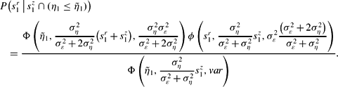
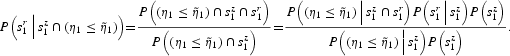
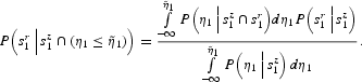
We first compute
. By repeatedly applying the definition of conditional probability, we obtain
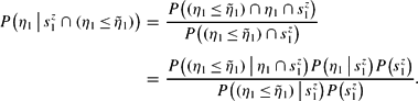
Exploiting the fundamental lemma on conditional probability (see, e.g., Grimmet and Stirzaker, 1992), we obtain
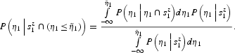
Hence,

We now compute
, which is the probability that agent r receives a specific signal (
given that agent z has received signal
and that
. As before, we apply the definition of conditional probability, obtaining
Hence, exploiting the fundamental lemma on conditional probability (see, e.g., Grimmet and Stirzaker, 1992), we get
The joint normality of
, and
allows us to conclude that