Introduction and historical context

This paper describes a system, moth imaging system (MIS), developed in 1982, to image and automatically analyze the trajectories of moths in flight around artificial sources of illumination under field conditions (Gaydecki, Reference Gaydecki1984). The work was conducted as part of a research programme at the Ecological Physics Research Group, Cranfield Institute of Technology, UK (now Cranfield University). The investigation was never published and as far as is known, the analysis that resulted from the fieldwork data remains unique. The technique, based on computerized analysis of an individual moth's digitized track data in combination with simultaneously acquired wind speed and direction data, enabled a detailed picture of flight patterns to be constructed; further, a numerical model was developed using an ensemble of a large number of tracks, which accurately predicted the flight density profiles around light sources typically used in light traps. The research sought to address questions concerning light trap influence on moth flight behaviour, about which, at that time, very little was known with certainty. These included trap efficiency, the range of influence, close-range flight behaviour, phototaxis and the effects of meteorological conditions on the trajectories. Neurobiological explanations for phototaxis were deliberately avoided; rather, quantified descriptions of behavioural change (i.e. trajectories and deviations), in addition to patterns in ensemble distributions, formed the focus of much of the analysis.

The MIS research was founded on earlier work conducted in the 1980s, in which a system known as IRADIT (Infra-red Active Determination of Insect Flight Trajectories) was developed to image remotely small insects flying above a crop canopy during daylight hours (Schaefer & Bent, Reference Schaefer and Bent1984). It is important to emphasize that MIS, which was deployed for nocturnal insect imaging, is distinct from IRADIT (although they were developed in the same department); however, both used an active form of illumination as the source.

Passive observation involving a detector (either the human eye or an imaging system) relies upon sufficient contrast between the insect and the background. In most cases, the signal-to-background ratio (SBR) will be inadequate for distances greater than a couple of metres, since reflections from insect wings will generally be no greater, or even weaker, than the visible energy reflected from the crop, or the ambient illumination from the daytime sky. Under certain situations, the contrast is, however, favourable – for example, when observing hoverflies in a shaft of sunlight within a woodland setting. In this case, specular reflections (reflections from optically smooth surfaces) from the wings enhance the contrast. If the insect is positioned between the source and the detector, forward scattering (scattering towards the detector and away from the source) further enhances the SBR through diffraction and refraction. This effect is most noticeable, for example, when observing fine rain droplets at night, caught in the beam of a vehicle's headlights located in front of the observer.

Calculations confirmed that neither for IRADIT nor MIS, passive detection would yield an acceptable SBR, so active solutions were sought. We do not describe in any detail here the technical aspects of IRADIT (which, in any case, are provided elsewhere) since it is not the subject of this paper. Suffice it to state that IRADIT employed a powerful, pulsed infrared beam at a wavelength in which the sun is deficient. When shone over a crop, any insects present within the intersection volume of the beam and field-of-view of an image intensifier/video camera tuned to this wavelength were revealed as bright points of light on an otherwise dark background.

In contrast, MIS used a mercury vapour light as both the attractant and the active source for the image intensifier/video camera, which generated 50 images, termed fields, per second. The light was mounted on a mast at heights of either 5 or 7.1 m (depending on the experiment), with the camera and associated optics positioned at the base of the mast, looking upwards. Over several nights in early September 1982, hundreds of moth flight tracks, together with meteorological data, were transferred to a computer and analyzed automatically by software. Accumulated density profiles of the track data revealed that at low wind speeds, moths spend most of their time at a radius between 40 and 50 cm from the source, and rarely fly directly above it, from close range. This profile skews as the wind speed increases but does not fundamentally alter until the wind speed exceeds the maximum flight speed, in still air, of the moth. The proportion of insects caught by the trap in comparison with the number within the field of view of the camera was very low; of 1600 individual tracks recorded over five nights, a total of only 12 moths were caught. Although trap efficiency is strongly influenced by environmental factors, the analysis confirmed that moths do not exhibit straightforward positive phototaxis. In general, trajectory patterns become more complex with reduced distance from the illumination, with speed, acceleration, deceleration and angular velocity inversely related to distance from the light. The highest accelerations also tended to occur when the insect was at close range but moving away from the source. Rather than manifesting a simple positive phototaxis, the trajectories were suggestive of disorientation. Arising from the density profile analysis, mathematical models based on the concept of competing negative and positive phototaxis were developed. These described ideal density distributions in calm air and light wind speed conditions. The models did not offer a physiological hypothesis regarding the behavioural changes, but rather were tools for quantification and prediction. The qualification offered by this latter point is significant. The model was pragmatic rather than explanatory, and whilst under certain limited meteorological conditions it was a useful statistical tool for predicting moth densities in the region around artificial light under field conditions, it did not provide a deeper understanding of insect behaviour, based on physiological responses, in any rigorous manner; neither was it intended for this purpose.

Since that time, the tools available for both imaging and analyzing insect flight patterns have become more powerful, smaller and of course cheaper (El-Sayed et al., Reference El-Sayed, Gödde and Arn2000; Reynolds & Riley, Reference Reynolds and Riley2002; Sokolowski et al., Reference Sokolowski, Moine and Naassila2012; Whitehorn et al., Reference Whitehorn, Hawkes and Dublon2013). A revised system is now undergoing development, employing the latest infrared laser technology and automated tracking software, but based on the same principles established in the original 1982 study, to analyze a range of insects, including bees and pestiferous species, during daytime flight.

Fieldwork design and equipment

The fieldwork equipment for the moth imaging study was located on a secluded perimeter path of the main aircraft runway operated by Cranfield University; this path runs adjacent to a field which had been used to cultivate a wheat crop. All field work was conducted between 20.45 and 22.00 BST on the evenings between 6 and 11 September 1982. By this time in the year, the crop had been harvested and the stubble burned.

Illumination and imaging

The imaging of moths at night flying in the vicinity of an artificial source – a mercury vapour light bulb – represented a straightforward challenge for the detection and imaging system, since a good contrast between the illuminated wings and the dark sky was assured. The mercury vapour bulb hence acted as both the phototactic agent and the source of illumination for the camera. However, because of the fieldwork configuration (described below), the moths reflected the light through side scattering rather than forward scattering, which is necessarily less efficient. In addition, the reflection from moth wings is diffused rather than specular (since their surfaces are textured rather than membranous and reflective), further reducing the energy arriving at the lens. For these reasons, it was necessary to use an electronic image intensifier located between the lens and the camera.

The field work equipment is shown in fig. 1 and is now described in detail. The only part of a Robinson light trap of significance to this work was the conical centre section bearing the 125 W mercury vapour bulb and the horizontal baffles. This part of the trap, which included a modified base to accept a collecting bottle, was secured by means of a horizontal metal arm 0.5 m in length to a Clark pneumatic mast, in such a manner that no light was cast upon the mast or surrounding equipment. The topside of the trap was silvered to reflect the light from the bulb, but the underside was painted matt black to ensure that no stray light was detected by the imaging system. Once the trap was raised off the ground, the angle through which light was cast was 2.3 steradians. The camera and intensifier were mounted on a solid aluminium base plate and positioned horizontally at the foot of the mast, with a mirror angled at 45°, enabling the camera to receive an image of the light-trap in plan view. As the night-time temperature fell, condensation formed on the mirror; this problem was solved by constructing a low-voltage heating element and attaching it to its back face. Two sample heights were used: 5 m (6 and 8 September) and 7.1 m (9, 10 and 11 September). To obtain as wide a field of view as possible, a 17 mm focal length wide angle lens was coupled to the intensifier. On the rectangular monitor screen, this gave a view angle of 37° from left to right and 28° from top to bottom. At a height of 5 m, the visible area was 3.8 × 2.6 m² and for 7.1 m it was 5.3 × 3.6 m². To facilitate data interpretation, the camera and mast were aligned so that the top of the screen always pointed towards magnetic North.

Fig. 1. Fieldwork configuration of moth tracking study, September 1982. The system comprised: (a) the pneumatic telescopic mast; (b) two vane anemometers mounted orthogonally (facing N/S and E/W); (c) 125 W mercury vapour lamp, including baffles and a collection bottle; (d) electrically heated mirror angled at 45°; (e) wide-angle lens; (f) electronic image intensifier; (g) video camera.

Computation and instrumentation summary

Information collected in the field, i.e. video of moth light tracks and wind vectors, were ultimately converted into digital form and transferred to a computer for storage and analysis. In 1982, the processing power available to many small university departments conducting ecological research was rather limited. In this case, the entire data analysis was performed by an Apple II personal computer that featured 64 kb of memory and an 8-bit processor with a clock speed of 1 MHz. No programs of any kind were available for data acquisition, storage, processing, display or interpretation. A major aspect of the research required the development of software for these purposes; because of the limited power and capacity of the computer, much of this was written using a combination of both BASIC and pure assembly code. Since the operating system consumed approximately 16 kb, only 48 kb were available to hold the programs written for the project. Assembly was used when necessary since it resulted in very compact code; although it is tedious to write and difficult to maintain, the constraints of the hardware dictated this approach. Additionally, the acquisition, display and processing programs were written as separate executables and loaded as required – capacity did not permit a single unified package. Full details are available from the thesis (Gaydecki, Reference Gaydecki1984).

Track data transfer: the light pen

Extraction of the track data into coordinate pairs was rather more challenging. The video was generated at 50 fields per second (following the PAL standard) and stored on analogue video tape. Within each field, the only information of significance was the moving points of light that represented the flight tracks of each moth. A novel solution for coordinate extraction was developed in the form of a light pen interface, which performed the direct transfer of tracks on the video recorder monitor to a computer for storage and processing. Using freeze-frame mode, the video was advanced field-by-field; with each new field, the operator positioned the light pen at the head of the selected track and pressed a key. The circuitry would then extract the coordinates of the light pen's current position and transfer this to the computer.

The operating principle of the light pen exploited the manner in which video images are produced and in particular, the synchronization signals of the video monitor; in the PAL standard, each TV frame comprises 625 horizontal lines, generated at 25 Hz. A frame is further subdivided into two fields, each of 312.5 horizontal lines. The lines of the second field are offset to lie between the lines of the first in a scheme known as interlacing. Lines are produced by an electron beam that scans across and down the face of the cathode ray tube (CRT); this beam is controlled in its movement by the CRT's X and Y deflection plates, which pull the beam from left to right in 64 microseconds and from top to bottom in 20 ms. The light pen circuitry sampled the deflection plates’ X and Y synchronization signals and used them to generate linear X and Y voltage ramps. When the light-pen was placed over a bright region of the screen, the photodiode at its tip produced a pulse that instructed the circuitry to sample the instantaneous voltage of the ramps at that moment in time. Because the ramps of the light-pen were synchronized to the monitor, the sampled voltages corresponded to the coordinate position of the pen. These were then digitized and fed to the computer. Not all tracks were digitized; some were out of focus, too faint or short and contained insufficient information (<0.2 s). Of 1600 tracks imaged, 419 were usable. This represented 536.88 s of track data, i.e. 26,844 fields of video (pairs of flight coordinates). A practised operator could process one frame approximately every 3 s, requiring a total of 22.37 h of effort. The procedure, conducted in a darkened room, was rather fatiguing and necessitated frequent rest breaks to ensure consistency. The acquisition process was therefore spread over a period of approximately 10 days. A photograph of the light pen equipment is shown in fig. 2, and the complete instrumentation system in fig. 3.

Fig. 2. The light pen instrumentation, comprising light pen electronics (bottom left), video recorder, video monitor and Apple II computer.

Fig. 3. The complete laboratory system, comprising the meteorological processor, FM tape recorder, digital interface, video tape recorder, monitor and light pen unit. All digitized data were ultimately transferred to the computer.

Trajectory analysis and density profiling software

Once the flight tracks had been acquired, they were converted to represent actual distances using a conversion factor based on the field of view of the video monitor and its distance to the source. Similarly, the binary wind data were expressed as wind speeds. Following this stage, a control system was written that provided synchronization between the wind and track data. Four analysis programs were written to process the digitized insect video data. The first performed trajectory analysis for each individual track; the other three programs accumulated density profiles, and mapped them according to the area, distance or angle subtended from the light. They are described as follows.

1. 1. Trajectory analysis: The program averaged the position of each insect over five readings (taken at 50 Hz) to produce a temporal resolution of 0.1 s. This reduced the scatter associated with the acquisition process and gave greater reliability to the movement statistics. It generated the following statistics for each track: mean, minimum and maximum ground speed, maximum acceleration and deceleration and maximum angular velocity. Next, it divided the visual field into a grid of 10 × 10 cells. This arrangement is shown in fig. 4, which also includes the digitized trajectory of a moth. At a height of 5 m (measured from the light to the mirror), the area of the visual field was 3.8 × 2.6 m². Hence each cell area was 0.38 × 0.26 m². At a height of 7.1 m, each cell area was 0.53 × 0.36 m². It then matched each velocity measurement with its corresponding grid reference, distance from the light, flight heading, wind speed and direction (except for the mean velocity). The program then subtracted the wind vectors to calculate the airspeeds of each insect. The program next divided the visual field into a series of concentric annuli centred around the light, 0.25 m in width, and calculated how much time the insect spent within each annulus. Finally, it computed the history of each trajectory, mapping speed and distance as functions of time. These statistics were useful because they lent circumstantial support to the disorientation hypothesis, described below. A typical output table from the trajectory analysis program is shown in table 1, which tabulates trajectory statistics for a single moth track.

2. 2. Density profile vs. area: This program divided the field of view into a more highly resolved grid comprising 28 × 19 cells. Each cell was square, with sides of 0.14 or 0.19 m depending on whether the elevation was 5 or 7.1 m respectively. This allowed a track density profile to be generated of the area within the field of view of the camera.

3. 3. Radial density profile: This program divided the visual field into a series of concentric annuli centred around the light, each of 0.05 m width, and produced a histogram for accumulated time spent in each annular area.

4. 4. Angular density profile: This program divided the visual field into sectors in 6° increments and produced a histogram for accumulated time spent in each sector. This information was used to inform the model with respect to cosine dependency of the density in relation to wind speed and direction.

Fig. 4. Typical digitized moth track (camera view), with the light source denoted by the solid black circle.

Table 1. Output generated by FLITRAP for a single moth track.

The statistical measures of the movement were subject to two principal sources of error. The first arose due to the depth of field of the lens. Although the optical system was designed to have a depth of field of 0.5 m, located at the horizontal plane of the light, moths could nevertheless be imaged above and below this exact distance. At a camera distance of 5 m, this resulted in an irreducible velocity measurement uncertainty of approximately ±5%. As far as possible, the further error was minimized by rejecting out-of-focus tracks. The second source of error arose from the digitization process. Ideally, the light pen should have been located at the very head of the track, but the nature of the manual process limited the accuracy; For this reason, track data points were averaged.

Qualitative interpretations and statistical summary

Figure 5 is a freeze-frame photograph taken from the original video data. It shows a moth veering sharply away from the trap, the position of which is indicated by the red circle (drawn to correct scale). In this image, the camera is looking vertically upwards, with the light at an elevation of 5 m. Examination of the moth track reveals a regular pattern of modulation produced by the beating of the wings. The impression given by visual inspection of such data was one of apparent disorientation (the definition of disorientation is used without prejudice and it is not intended to imply anything concerning the insects’ internal state). One commonly encountered pattern involved sinusoidal flight towards the source, often becoming more exaggerated and with greater speed changes, until at some point the moth was caught, or more usually, flew rapidly away. Helical spiralling flight along the axis of movement was also observed. Although this pattern was the most often encountered, most tracks usually incorporated a variety of movements, for example, helical flight switching to sinusoidal weaving. Circling of the lamp was also observed but it was not common, accounting for 2% of all tracks analyzed. This behaviour is often said to occur with moths flying around domestic light bulbs, so the patterns of flight may have been influenced by the condition of the environment.

Fig. 5. Video freeze-frame, showing a moth turning sharply away from the light trap, indicated by the circle.

Table 2 summarizes the trajectory statistics generated by the software for all nights, with standard deviations given in parentheses (except for the final column, where the figures in parentheses denote significance). These include mean, minimum and maximum ground speeds and maximum accelerations, decelerations and angular velocities averaged over each night, together with the distances from the trap at which the maxima and minima occurred. Maxima and minima tend to occur at close range, rather than when the moths entered the field of view. It is reasonable to hypothesize, therefore that the flight behaviour is, ostensibly at least, characterized by disorientation at close range. As a caveat, it should be stated that no neurobiological studies have been conducted to support this description.

Table 2. Averaged nightly ground speeds, accelerations and angular velocities.

SI units throughout.

The variations in flight dynamics in the vicinity of the light relate specifically to rapid fluctuations in flight vectors (measured accelerations, decelerations and angular velocities). These were in general inversely related to the distance from the light source. This was established by the trajectory analysis software in the following manner. For each moth track, it calculated the maximum acceleration, deceleration and angular velocity, and the distances at which each of those values occurred. It then performed regression analysis for the three parameters as a function of distance. In all three cases, the slope was negative. For the night of 6 September for example, the relationship between maximum speed v and distance r was calculated to be:

(1)$$v = 3.71 - 0.54r$$

This relationship only held true within the field of view of the system. Although some maximum ground speeds occurred inside a radius of 0.2 m, as well as some of the highest accelerations, no deceleration was recorded at a distance <0.3 m – at such close range, it might be concluded that negative phototaxis was dominating the flight behaviour.

To explore the complexity of the phototactic response, the program also computed approach data, shown in the final column of table 2. It revealed that for approximately 70% of the moths, the lowest speeds were recorded as they flew towards the light, i.e. a positive approach. All of the approach data statistics were statistically significant below 0.05, as indicated by the figures in parentheses. At the very least, this suggests that positive phototaxis is not the sole factor in influencing dynamic flight strategy.

A question naturally arises as to whether all of the insects imaged and tracked were moths. This is difficult to answer with certainty, but circumstantial evidence suggests that this was the case for the sizeable majority. As stated above, over the course of five nights only 12 insects were caught in the collection bottle, and these were all Lepidoptera. The previous year, trapping had been conducted in the same vicinity, but at ground level, over 19 nights, between the hours of 20.30 and 03.30 BST, with the catch counted every 30 min. The results are not reported in detail here, but again the significant majority were moths. Perhaps most important, the form and brightness of the tracks were consistent with the signatures that would be expected from these insects.

The area density profiles for 6 and 8 September are shown in figs 6 and 7. The profiles were obtained in the following manner: the program scanned each cell in the grid and summed all of the track points that occurred within it. The height of any given cell in the profiles plotted on the z-axis, corresponds to its accumulated total. This was a compute-intensive task, but entirely automated. These profiles suggest that the density rises from the periphery of the field of view, reaches a maximum at some distance from the trap, and then falls almost to zero directly over the region of the light source. Further, the distribution is skewed by the wind speed and direction, which averaged 0.85 ms⁻¹ over the two nights. This skew corresponds to the prevailing wind direction, with moths aggregating downwind of the light. The radial density profiling program (described above) then accumulated the track points in each annulus and divided the total by the area to obtain density. Figure 8 shows the normalized radial density profile for 6 September. Normalization was performed by dividing the absolute value of each reading in the radial density profile by the largest value (which, for fig. 8, occurred at a distance of 0.4 m). Normalization allowed meaningful comparisons of profiles taken on different days to be made and simplified the development of the model, given below. It confirms clearly that the density rises sharply to a peak at a distance between 0.4 and 0.5 m from the trap and decays nearly to at a distance of 2 m.

Fig. 6. Area density profile for 6 September. Solid black circle denotes light source. Grid is 3.8 × 2.6 m². The profile was obtained by summing of the track points within each cell (see text).

Fig. 7. Area density profile for 8 September. Solid black circle denotes light source. Grid is 3.8 × 2.6 m².

Fig. 8. Radial density profile for 6 September.

Data interpretation and modelling

A model was developed to predict relative density profiles based upon the hypothesis that moths manifest positive phototaxis, i.e. they are attracted to light in addition to an escape response, manifesting as negative phototaxis, which observations suggested dominated flight behaviour at close range to the source. This model did not attempt to explain the nature or provenance of moth flight behaviour; neither did it hypothesis about the neurological basis of the phototactic mechanism. Rather, it was an empirical tool employing a number of arbitrary coefficients, the values of which were found through data fitting. It did not calculate absolute estimates; neither did it account for the elevation of the light nor its luminosity. These factors could, in principle, have been incorporated into the model but data collection was constrained by the season and equipment limitations. Despite its ad hoc nature, it provided an accurate quantitative description of distributions around the light source in both calm and moving air. Its key assumptions were: the strength of both of the attraction response (positive phototaxis), R _a, and the escape response (negative phototaxis), R _e, diminished exponentially with distance, as the apparent luminosity weakened (a caveat to this assumption is that relative angular change subtended at the moth's eye respecting the light will also diminish, a factor not accommodated by the model); further, the responses reach a finite maximum, at zero range, since the absolute luminosity is finite. Finally, the response must satisfy the inverse relationship between light intensity and distance, i.e.

(2)$$R_a = {\rm e}^{ - (r^{\rm \lambda} /a)};\,\,\,R_e = {\rm e}^{ - (r^{\rm \lambda} /b)}$$

It is important to emphasize that this is not a behavioural model and cannot be applied to individual insects; rather, it predicts the density profile of a large number of moths within the immediate vicinity of the light used in these experiments.

In the past it was hypothesized that migratory moths misinterpret the artificial light as the moon (which they employ as an orientation cue), and react by attempting to maintain a constant angle with respect to its image. At a large distance from the source, the angles of elevation and azimuth that the light subtends at the eye of the moth changes little as the moth moves, and the energy flux is low (Baker & Sadovy, Reference Baker and Sadovy1978; Sotthibandhu & Baker, Reference Sotthibandhu and Baker1979). At 500 m for example, the energy flux from a 125 W MV bulb in the 500–600 nm band is equivalent to that from the full moon. In recent years this transverse orientation theory has rather fallen out of favour, but still has its proponents (see Commentary below). Whether or not it is a valid explanation, as a moth nears the source, other factors start to dominate that confirm the light is not the moon: the angle subtended at the eye alters quickly as the animal moves, the elevation is variable and most importantly, the energy flux increases. Hence R _e. begins also to increase; unlike R _a, it appears later but when it does it grows more rapidly. Since R _e is antagonistic with respect to R _a the combined response is R _a–R _e. As a moth nears the source under the predominant influence initially of R _a there a should be little to indicate any disorientation in the flight path. Thereafter as R _e increases with shortening distance from the light, the moth begins to reduce its speed, i.e. minimum speeds should take place during the approach phase. At a certain radius from the trap the combined response reaches a peak, representing the point of dynamic equilibrium. Movement either towards or away from the light causes a reduction in the strength of combined response, such that the moth seeks to maintain this optimum radius. Because of the instabilities induced by local wind vectors and the moth's own inertia, as well as the energy required for hovering flight, its movements will oscillate about this point of stability. Further, the rapid fluctuation of the responses will cause the moth to fly in an erratic manner, quite atypical to its normal flight strategy.

Figure 9 shows the combined radial density profiles of 6 and 8 September overlaid with the density prediction d _r (dotted line), obtained using the model in calm air:

(3)$$d_r = k[{\rm e}^{ - (r^{\rm \lambda} /a)} - {\rm e}^{ - (r^{\rm \lambda} /b)}]$$

In which λ = 1.62, a = 1600, b = 320 and k is the constant of proportionality depending on the absolute number of track points. The figure suggests the model yields an accurate estimate of the density profile, with R = 0.97 (P < 0.001). By rotating the model about the z-axis, it is possible to generate the area density profile for moth flight tracks under calm conditions (fig. 10).

Fig. 9. Combined radial density profiles for 6 and 8 September, overlaid with model fit.

Fig. 10. Ideal moth density profile in calm conditions. Area is 2 × 2 m².

The direction and strength of the wind strongly influence the density profile; data analysis revealed that in light wind, the angular density profile is cosine dependent, as indicated by fig. 11, which plots distribution as a function of angle in 6° increments, for 6 September. The inclusion of a cosine term in Equation (3) allows the area density profile to account for this parameter, i.e.

(4)$$d_r = k\,(1 + v\cos {\rm \theta} )\,[{\rm e}^{ - (r^{\rm \lambda} /a)} - {\rm e}^{ - (r^{\rm \lambda} /b)}]$$

In which wind speed and direction are denoted by v and θ, respectively. Figure 12 shows an output from the revised model, in which the wind speed is 0.8 ms⁻¹ with a compass bearing of 180°. The model is only valid for wind speeds less than the maximum ground speed of a moth – above this value, the moth cannot delay in the vicinity of the trap but will be dragged by the flow of the wind.

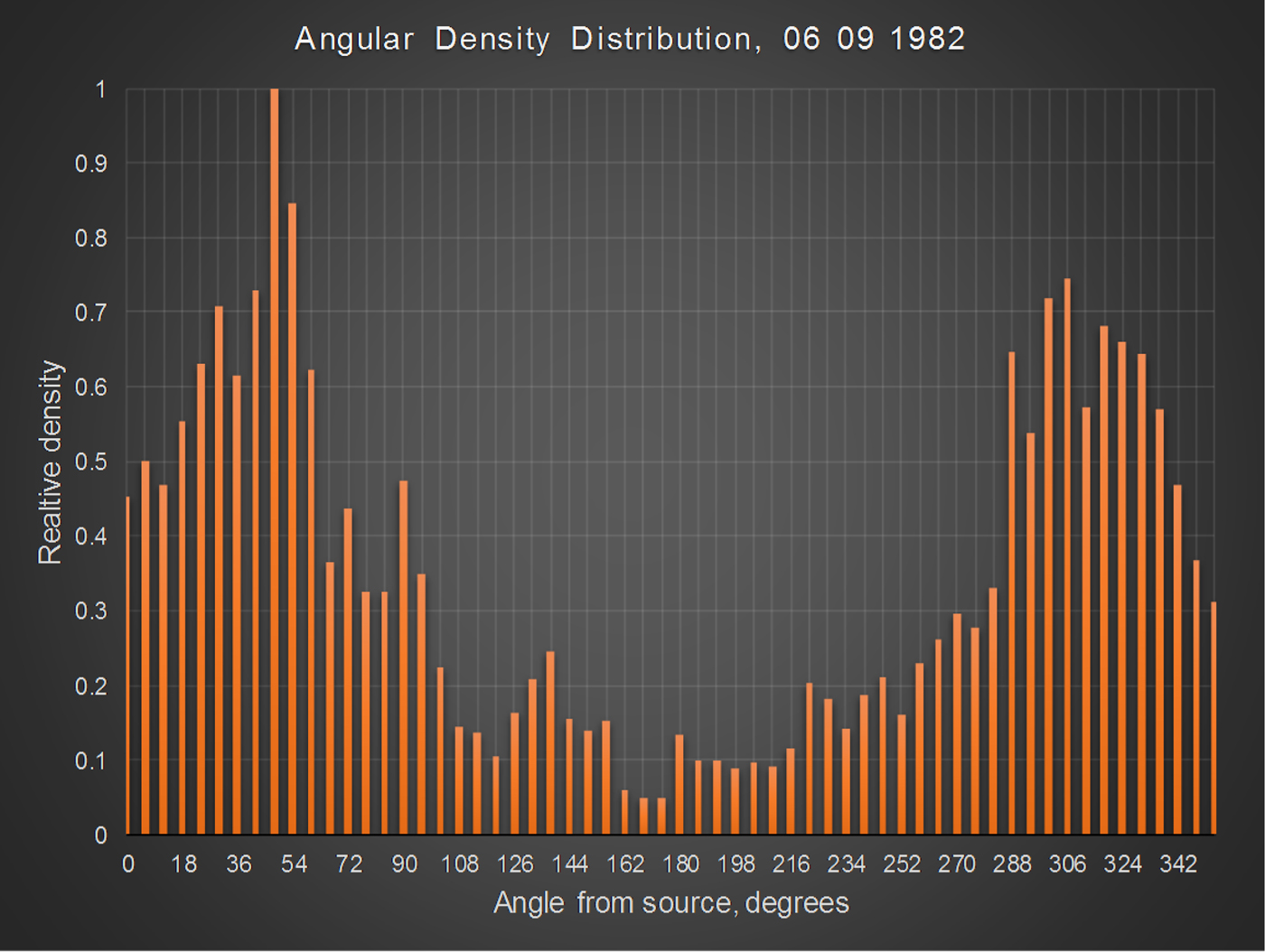
Fig. 11. Moth density profile as a function of angle subtended at the source for 6 September.

Fig. 12. Ideal moth density profile in light wind conditions. Area is 2 × 2 m².

As an example of this limitation, an attempt was made to fit the revised model to the radial density profile for 9 September, for which the mean wind speed over the course of the experiment was 1.7 ms⁻¹. The angular density profile and model fit is shown in fig. 13. Although the curve follows the general trend, the error is greater with R = 0.93 (the data also suggest the possibility of overlapping populations, but this is impossible to verify retrospectively). No attempt was made to apply the model to the data collected on the 10 and 11 of September, for which the mean wind speeds were in excess of 2 ms⁻¹.

Fig. 13. Radial density profile for 9 September, overlaid with model fit.

System evolution and new applications

The technology for tracking the migration patterns of insects has evolved since the 1980s and is now of central importance to understanding spatial population dynamics and in analyzing the impact of insecticides (such as the newer neonicotinoids) on honeybee and bumblebee populations, crop pollination activity and optimization of hedgerows and set-aside field margins as feeding and breeding sites for pollinators.

At the macro-scale, this need is addressed with entomological radar (Mueller & Larkin, Reference Mueller and Larkin1985), which is a mature and well-established technology. However, conventional radar of this kind (typically vertical-looking radar, or VLR) cannot image targets closer than 150 m (the dead zone) and certainly cannot track or image individuals within a swarm. Radar is an excellent tool for tracking large migrating swarms of insects (Smith et al., Reference Smith, Riley and Gregory1993) but is less suitable for recording and analyzing the movements of insects over a crop or orchard, which would, in any case, contribute to an intolerable level of radar clutter artefact through microwave backscatter.

A variant of this technique termed harmonic radar (Psychoudakis et al., Reference Psychoudakis, Moulder, Chen, Zhu and Volakis2008), may be used to track individual insects and has been intensively explored by Rothamsted Research UK (Riley et al., Reference Riley, Smith, Reynolds and Edwards1996). A small passive transponder, weighing a few milligrams, comprising a Schottky barrier diode with a wire antenna, is attached to the thorax of the insect. A conventional radar transmitter fires a tone burst, typically in the frequency range of 1 GHz. When this interacts with the transponder, the diode performs a full wave rectification of the signal and re-radiates a waveform at double the frequency. This is then received and amplified, allowing the insect to be ranged and tracked. Harmonic radar is useful for studying selected, individual migratory behaviour but cannot be used to track field populations of bees; further, it is limited to the larger insects.

Video imaging and trajectory analysis of insects is now a widely investigated area; however, in many cases, it is confined to close range observations with restricted fields of view. Wilkinson et al. (Reference Wilkinson, Lebon, Wood, Rosser and Gouagna2014) describe a sophisticated camera and forward-scattering illumination system that can track and separate multiple mosquito targets, but the experiments were conducted indoors using a flight chamber considerably smaller than 1 m². Angarita-Jaimes et al. (Reference Angarita-Jaimes, Parker, Abe, Mashauri, Martine, Towers, McCall and Towers2016) have similarly developed a mosquito tracking system that employs a flight chamber and forward scattering configuration, but the inclusion of a Fresnel lens in the optics enabled a clearly defined object volume to be illuminated. Mullen et al. (Reference Mullen, Rutschman, Pegram, Patt and Adamczyk2016) extend this concept, incorporating a laser system not only to image mosquitos at close range but also to eradicate targets with a lethal pulse of infrared laser energy. Laboratory-based video insect tracking systems are indeed relatively common, in particular for characterizing bee behaviour (Ingram et al., Reference Ingram, Augustin, Ellis and Siegfried2015), but in the field, in uncontrolled conditions, there is far less research reported in the literature. In contrast, very sophisticated systems have been developed for tracking larger animals including bats and bids. A notable example is the work conducted by Evangelista et al. (Reference Evangelista, Ray, Raja and Hedrick2017), in which three high-speed DSLR cameras, mounted along a 9 m baseline and at different heights, were used to characterize 3D trajectories of chimney swift flocks within a target volume of 833,000 m³.

Due perhaps to their size, there is a paucity of methods for tracking insects at the mesoscale, in which the field of view is typically <100 m² and located no more than 100 m to the target zone. This is now being addressed with a proof-of-principle system that has been developed to image and analyze remotely the flight trajectories of bees under field daylight conditions, based on the original moth work; this will be described in a future publication. It comprises a compact infra-red laser source mounted in a steerable frame and a high-speed video camera incorporating a low-pass 780 nm infra-red filter, operating at 350 frames per second. The camera downloads the video in real time to a computer via a high-speed USB 3 link, where the data are automatically analyzed by software in real time; crucially, the software is capable of identifying tracks automatically without the need for operator intervention. The system weighs less than a tenth of the original IRADIT and MIS systems, the processing system is orders of magnitude more powerful and the cost is a small fraction of the original.