


NOMENCLATURE
- ϕ
-
velocity potential function
- ∇2
-
laplace operator
- n
-
normal vector of the body's surface
- dS
-
elemental surface area
- μ
-
doublet strength
- σ
-
source strength
- B
-
influence coefficient of a unit source strength
- C
-
influence coefficient of a unit doublet strength
- CL
-
lift coefficient
- CD
-
drag coefficient
- CM
-
moment coefficient
- CT
-
propeller thrust coefficient T/ρπΩ2 R 4
- L/D
-
lift to drag ratio of the wing
- Cp
-
pressure coefficient
- N
-
number of vortex particle
-
 ${N_{\bm B}}$
-
number of body surface panel
- Nw
-
number of wake surface panel
- SB
-
body surface
- Sw
-
wake surface
- R
-
propeller or rotor radius
- Rn
-
dimensionless distance
-
${{\bm V}_0}$
-
free-stream velocity
-
${\bm u}$
-
local fluid velocity
-
${{\bm u}_{{\rm{ind}}}}$
-
induced velocity of a vortex particle
- vref
-
kinematic velocity
- ΔSk
-
body panel area
- ΔFk
-
aerodynamic force on the kth panel
- ρ
-
density of air
- Ω
-
the rotational speed of the body's frame of reference
- ςε
-
gaussian distribution function
- Δt
-
time step
- ω
-
vector vorticity
- ν
-
kinematic viscosity coefficient
-
${\bm a}$
-
vorticity of particle
- ε
-
smoothing parameter
- V q
-
induced velocity of particle
- γ
-
surface vorticity


1.0 INTRODUCTION
The research on distributed electric propulsion (DEP) aircraft, such as solar-powered aircraft, has been motivated in recent years because of the beneficial increase in reliability, safety and total efficiency, and significant reductions in noise as well as system-level emissions. However, the distributed propellers’ rotation will make a large part of an aircraft's wing immerged in the propeller slipstream, such as the Helios prototype solar-powered aircraft(Reference Noll, Ishmael, Henwood, Perez-Davis, Tiffany, Madura, Gaier, Brown and Wierzbanowski1), whose propeller slipstreams cover more than 50% of the wing area. Distributed propeller slipstreams will cause mutual aerodynamic interactions between propellers and the wing, which can significantly affect the DEP aircraft's performance, stability and so on. Therefore, accurate and fast analysis is required to perform conceptual design for the DEP configuration and critical for avoiding the expensive modification at a later stage.
In recent years, the Computational Fluid Dynamics (CFD) technology has been successfully applied to numerically simulate the complicated flow for the propeller-driven aircraft or the rotorcraft. There are mainly three kinds of methods that have been developed, including the actuator disc method(Reference Thouault, Breitsamter, Gologan and Adams2 - Reference Thouault, Breitsamter, Gologan and Adams4), the Multiple Reference Frame method(Reference Hu, Ouyang and Du5) and the unsteady sliding mesh method(Reference Liu and Pan6,Reference Nicolas, Breitsamter and Adams7) . Although the CFD method has a high fidelity in predicting the propeller-wing interference behaviour, its computational cost limits its own applications at conceptual and preliminary design stages of an aircraft. In addition, using only an experimental method to address the effect of the interaction is also not a viable option because of its high cost. In order to overcome the above issues, methods and tools capable of rapidly and accurately predicting propeller slipstream effects are required.
Panel methods(Reference Richason, Katz and Ashby8 - Reference Degennaro10) have been widely used to predict aerodynamic forces of aircraft during initial design studies because of their computational efficiency. Although easy to use, most modern panel methods still have severe drawbacks. The main drawbacks are the inviscid assumption and the singularity problem which occurs when wake panels are close to each other(Reference Wie, Lee and Lee11). In addition, most panel-method implementations require the user's expertise and effort to specify wake positions. The unreasonable wake panel positions will result in unavoidable wrong calculation results. Therefore, the traditional panel method should be improved by combining another wake dynamic method to simulate complex wakes.
The free-wake method(Reference Leishman, Bhagwat and Bagai12) is often coupled with the panel method to simulate the complex wakes of the rotor or the propeller by replacing the wake panels with vortex lattices; however, its result depends on empirical formulations such as the vortex decay factor or vortex core size and therefore its applications are also limited.
Compared with the free-wake method, the vortex particle method is a powerful numerical tool to solve the flow around the complex geometries. The wake of the lifting surface is modelled with vortex particles(Reference Huberson, Rivoalen and Voutsinas13) and there are fewer empirical parameters. This approach has been combined with a panel method to predict the aircraft's aerodynamic forces(Reference Huberson, Rivoalen and Voutsinas13 - Reference Willis, Jaime and Jacob16). However, the flow viscosity effect is neglected in these studies.
In this paper, a panel/viscous vortex particle hybrid method, considering the flow viscosity, is developed. The aerodynamic force on the body's surface is determined by the panel method while the wake surface shed by the trailing edge of the wing is described using the viscous vortex particle method. In order to establish the relationship between the panel and the vortex particle method, the procedure of converting a wake panel doublet to a vortex particle vorticity is necessary and important. In addition, the influence of the wake vortex particle on a body panel is also implemented according to the Neumann boundary condition.
The present study analyses the wing aerodynamic behaviour under the influence of the propeller slipstream. As a first step, the panel/viscous vortex particle hybrid method is presented and the method validation is conducted by comparing with experimental results. As a further step, the propeller installed position, the propeller number and its rotational direction are discussed for two kinds of propeller-wing configurations, i.e. a tractor propeller configuration and an over-the-wing propeller configuration, to investigate the aerodynamic behaviour of the wing influenced by the propeller.
2. COMPUTATION METHOD
In this section, the panel method (Section 2.1), the viscous vortex particle method (Section 2.2) are described respectively. In order to establish the relationship between these two approaches, a Hess's demonstration is used to convert a doublet wake into a vortex wake (Section 2.3). In addition, the influence of the wake vortex particle on the body panel is considered and implemented by using the Neumann boundary condition (Section 2.4). Lastly, two wind tunnel models with experimental data are used to perform the method validation in Section 2.5.
2.1 Panel method
Consider a body with known boundaries moving in a potential flow which is irrotational, inviscid and incompressible, the continuity equation can be simplified to Laplace's equation( Reference Katz and Plotkin 17 ):
 $$\begin{equation}
{\nabla ^2}\phi = 0
\end{equation}$$
$$\begin{equation}
{\nabla ^2}\phi = 0
\end{equation}$$
where ∇2 is the Laplace operator, ϕ is a velocity potential function. According to Green's identity, the solution to Equation (1) can be constructed by a sum of source σ and doublet μ distributions on the known body boundary SB and the wake boundary Sw :
 $$\begin{equation}
\frac{1}{{4\pi }}\int_{{S_B}} {\mu {\bm n}} \cdot \nabla \left( {\frac{1}{r}} \right)dS - \frac{1}{{4\pi }}\int_{{S_B}} {\sigma \left( {\frac{1}{r}} \right)} dS + \frac{1}{{4\pi }}\int_{{S_w}} {\mu {\bm n}} \cdot \nabla \left( {\frac{1}{r}} \right)dS = 0
\end{equation}$$
$$\begin{equation}
\frac{1}{{4\pi }}\int_{{S_B}} {\mu {\bm n}} \cdot \nabla \left( {\frac{1}{r}} \right)dS - \frac{1}{{4\pi }}\int_{{S_B}} {\sigma \left( {\frac{1}{r}} \right)} dS + \frac{1}{{4\pi }}\int_{{S_w}} {\mu {\bm n}} \cdot \nabla \left( {\frac{1}{r}} \right)dS = 0
\end{equation}$$
where
 ${\bm n}$
is the normal vector of the body's surface and r is a distance between an arbitrary point in the flow field and its coordinate system's origin, and dS is the elemental surface area.
${\bm n}$
is the normal vector of the body's surface and r is a distance between an arbitrary point in the flow field and its coordinate system's origin, and dS is the elemental surface area.
2.1.1 Boundary condition
For a solid surface, there should be no flow flux penetrating it along its normal vector direction, which means a zero normal velocity on the boundaries should be specified. This direct formulation is called the Neumann boundary condition. According to this boundary condition, the source strength σ can be solved by
 $$\begin{equation}
\sigma = - {\bm n} \cdot {{\bm V}_0}
\end{equation}$$
$$\begin{equation}
\sigma = - {\bm n} \cdot {{\bm V}_0}
\end{equation}$$
where
 ${{\bm V}_0}$
is the free-stream velocity.
${{\bm V}_0}$
is the free-stream velocity.
In this paper, a constant strength rectilinear panel is assumed. After dividing the body and wake surfaces into
 ${N_{\bm B}}$
quadrilateral body panels and Nw
quadrilateral wake panels, Equation (2) can be transformed into the following form:
${N_{\bm B}}$
quadrilateral body panels and Nw
quadrilateral wake panels, Equation (2) can be transformed into the following form:
 $$\begin{equation}
\sum\limits_{k = 1}^{{N_B}} {{C_k}{\mu _k} + } \sum\limits_{w = 1}^{{N_w}} {{C_w}{\mu _w} + } \sum\limits_{k = 1}^{{N_B}} {{B_k}{\sigma _k} = 0}
\end{equation}$$
$$\begin{equation}
\sum\limits_{k = 1}^{{N_B}} {{C_k}{\mu _k} + } \sum\limits_{w = 1}^{{N_w}} {{C_w}{\mu _w} + } \sum\limits_{k = 1}^{{N_B}} {{B_k}{\sigma _k} = 0}
\end{equation}$$
where Ck , Bk are the influence coefficients of the panel k on an arbitrary point induced by a unit doublet strength and a unit source strength, respectively.
By using the Kutta condition, the unknown wake doublets μ w can be replaced by two corresponding unknown trailing-edge doublets μ u , μ l (“u” indicates the upper surface, while “l” the lower surface) of the wing:
 $$\begin{equation}
{\mu _w} = {\mu _u} - {\mu _l}
\end{equation}$$
$$\begin{equation}
{\mu _w} = {\mu _u} - {\mu _l}
\end{equation}$$
Substitute Equation (5) into Equation (4), Equation (4) can be rewritten as
 $$\begin{equation}
\sum\limits_{k = 1}^N {{A_k}{\mu _k} = - } \sum\limits_{k = 1}^N {{B_k}{\sigma _k}}
\end{equation}$$
$$\begin{equation}
\sum\limits_{k = 1}^N {{A_k}{\mu _k} = - } \sum\limits_{k = 1}^N {{B_k}{\sigma _k}}
\end{equation}$$
where Ak = Ck if the panel is not at the trailing edge of the wing; if it is, then Ak = Ck ± Cw .
2.1.2 Aerodynamic loads
When Equation (6) is solved, the source and doublet strengths of each panel can be obtained. Now, the pressure coefficient for each body panel can be computed as:
 $$\begin{equation}
{C_p} = \frac{{p - {p_{ref}}}}{{(1/2)\rho v_{ref}^2}} = 1 - \frac{{{u^2}}}{{v_{ref}^2}} - \frac{2}{{v_{ref}^2}}\frac{{\partial \phi }}{{\partial t}}
\end{equation}$$
$$\begin{equation}
{C_p} = \frac{{p - {p_{ref}}}}{{(1/2)\rho v_{ref}^2}} = 1 - \frac{{{u^2}}}{{v_{ref}^2}} - \frac{2}{{v_{ref}^2}}\frac{{\partial \phi }}{{\partial t}}
\end{equation}$$
where p and pref are the local pressure and far field reference pressure, u is the local fluid velocity, vref is the reference velocity and ρ is the density of the air.
In terms of the pressure coefficient the aerodynamic force ΔFk contributed by the kth body panel with an area of ΔSk is
 $$\begin{equation}
\Delta {F_k} = - {C_{pk}}{\left( {\frac{1}{2}\rho v_{ref}^2} \right)_k}\Delta {S_k}{{\bm n}_k}
\end{equation}$$
$$\begin{equation}
\Delta {F_k} = - {C_{pk}}{\left( {\frac{1}{2}\rho v_{ref}^2} \right)_k}\Delta {S_k}{{\bm n}_k}
\end{equation}$$
2.2 Viscous vortex particle method
2.2.1 Vorticity dynamics equation
In order to avoid the singularity problem mainly caused by wake panels, the vortex particle method(Reference Willis, Jaime and Jacob16,Reference Tan and Wang18 , Reference He and Zhao19) is used to model the vorticity in the wake domain. For an incompressible flow, the Navier-Stokes equation can be expressed in the velocity-vorticity form as follows:
 $$\begin{equation}
\frac{{\partial {\bm \omega }}}{{\partial t}} + {\bm u} \cdot \nabla {\bm \omega } = \nabla {\bm u} \cdot {\bm \omega } + \nu {\nabla ^2}{\bm \omega }
\end{equation}$$
$$\begin{equation}
\frac{{\partial {\bm \omega }}}{{\partial t}} + {\bm u} \cdot \nabla {\bm \omega } = \nabla {\bm u} \cdot {\bm \omega } + \nu {\nabla ^2}{\bm \omega }
\end{equation}$$
where ω is vector vorticity, ν is kinematic viscosity coefficient and
 ${\bm u}$
is the local fluid velocity.
${\bm u}$
is the local fluid velocity.
To solve Equation (9), the continuity vorticity field can be represented by the sum over all of the discrete vortex particles as:
 $$\begin{equation}
{\bm \omega }_\varepsilon ^h(x,t) = \sum\limits_{q = 1}^N {{{\bm a}_q}(t){\varsigma _\varepsilon }} [{\bm x} - {{\bm x}_q}(t)]
\end{equation}$$
$$\begin{equation}
{\bm \omega }_\varepsilon ^h(x,t) = \sum\limits_{q = 1}^N {{{\bm a}_q}(t){\varsigma _\varepsilon }} [{\bm x} - {{\bm x}_q}(t)]
\end{equation}$$
where N represents the number of vortex particle,
 ${{\bm a}_q}(t)$
and
${{\bm a}_q}(t)$
and
 ${{\bm x}_q}$
are the vector-valued vorticity and the position of the particle q, respectively, ςε is the Gaussian distribution function
${{\bm x}_q}$
are the vector-valued vorticity and the position of the particle q, respectively, ςε is the Gaussian distribution function
 $$\begin{equation}
{\varsigma _\varepsilon }({R_n}) = \frac{1}{{{{(2\pi )}^{3/2}}{\varepsilon ^3}}}{e^{ - R_n^2/2}}
\end{equation}$$
$$\begin{equation}
{\varsigma _\varepsilon }({R_n}) = \frac{1}{{{{(2\pi )}^{3/2}}{\varepsilon ^3}}}{e^{ - R_n^2/2}}
\end{equation}$$
where
 ${R_n} = | {{\bm x} - {{\bm x}_q}} |/\varepsilon $
is the dimensionless distance between an arbitrary point in the fluid field and the particle q and ε is the smoothing parameter.
${R_n} = | {{\bm x} - {{\bm x}_q}} |/\varepsilon $
is the dimensionless distance between an arbitrary point in the fluid field and the particle q and ε is the smoothing parameter.
When the continuity vorticity field is discretised by N vortex particles, the governing Equation (9) can be divided into two equations as follows:
 $$\begin{equation}
\frac{{\partial {\bm x}}}{{\partial t}} = {{\bm V}_0} + {{\bm u}_{{\rm{ind}}}}
\end{equation}$$
$$\begin{equation}
\frac{{\partial {\bm x}}}{{\partial t}} = {{\bm V}_0} + {{\bm u}_{{\rm{ind}}}}
\end{equation}$$
 $$\begin{equation}
\frac{{d{{\bm a}_p}}}{{dt}} = {{\bm a}_p} \cdot \nabla {\bm u}({x_p},t) + \nu {\nabla ^2}{{\bm a}_p}
\end{equation}$$
$$\begin{equation}
\frac{{d{{\bm a}_p}}}{{dt}} = {{\bm a}_p} \cdot \nabla {\bm u}({x_p},t) + \nu {\nabla ^2}{{\bm a}_p}
\end{equation}$$
2.2.2 Vortex stretching effect
In Equation (13), the first term in the right-hand side is called the stretching effect, which describes the vortex stretching and rotation due to the velocity gradient. In this paper, the so-called direct scheme method(Reference He and Zhao19,Reference Cottet and Koumoutsakos20) is used to solve this term:
 $$\begin{equation}
{\left. {\frac{{d{{\bm a}_p}}}{{dt}}} \right|_{ST}} = {{\bm a}_p} \cdot \nabla {\bm u}\left( {{x_p},t} \right) = \left[ {\nabla {\bm u}\left( {{{\bm x}_p},t} \right)} \right]\left[ {{{\bm a}_p}} \right]
\end{equation}$$
$$\begin{equation}
{\left. {\frac{{d{{\bm a}_p}}}{{dt}}} \right|_{ST}} = {{\bm a}_p} \cdot \nabla {\bm u}\left( {{x_p},t} \right) = \left[ {\nabla {\bm u}\left( {{{\bm x}_p},t} \right)} \right]\left[ {{{\bm a}_p}} \right]
\end{equation}$$
where
 $\nabla {\bm u}( {{x_p},t} )$
is the velocity gradient and its expression form is described in Reference He and ZhaoRef. 19.
$\nabla {\bm u}( {{x_p},t} )$
is the velocity gradient and its expression form is described in Reference He and ZhaoRef. 19.
2.2.3 Viscous diffusion effect
The second term in the right-hand side of Equation (13) represents the viscous diffusion effect, which describes the air viscosity through the vorticity transportation. This term, neglected in Refs (13–16), is considered in this paper and its solution can be derived using the particle strength exchange (PSE) method(Reference Eldredge, Leonard and Colonius21). The basis of this approach is using an integral operator to approximate the Laplacian operator, and the expression form can be written as
 $$\begin{equation}
{\left. {\frac{{d{{\bm a}_p}}}{{dt}}} \right|_{VDT}} = \nu {\nabla ^2}{{\bm a}_p} = \frac{{2\nu }}{{{{\hat{\varepsilon }}^2}}}\sum {{\varsigma _\varepsilon }\left( {{V_p}{{\bm a}_q} - {V_q}{{\bm a}_p}} \right)} \left( {{{\bm x}_p} - {{\bm x}_q}} \right)
\end{equation}$$
$$\begin{equation}
{\left. {\frac{{d{{\bm a}_p}}}{{dt}}} \right|_{VDT}} = \nu {\nabla ^2}{{\bm a}_p} = \frac{{2\nu }}{{{{\hat{\varepsilon }}^2}}}\sum {{\varsigma _\varepsilon }\left( {{V_p}{{\bm a}_q} - {V_q}{{\bm a}_p}} \right)} \left( {{{\bm x}_p} - {{\bm x}_q}} \right)
\end{equation}$$
where Vp and Vq are the volumes of particles p and q.
2.3 Conversion of doublet wakes to vortex wakes
The vortex-particle method is used to determine the wake domain vorticity after the potential flow on the body has been solved using the panel method. In order to establish the relationship between these two approaches, a procedure of converting double wakes to vortex-particle wakes is indispensable.
The wake model shed by the body trailing edge is composed of two parts: a doublet buffer wake sheet and a vortex-particle vortex(Reference Tan and Wang18) (see Fig. 1). The doublet buffer wake sheet is shed from the trailing edge of a lifting surface, and it has the same amount of panels as the trailing edge along the wing spanwise direction. In the streamwise direction, there are two rows of panels in the buffer wake sheet. The first row, which has a length of 0.3UΔt (Reference Willis, Jaime and Jacob16), is adjacent to the lifting-surface trailing edge and its doublet strength is determined by the Kutta condition. It is assumed that wake panels in the first row have constant doublet strength when they travel to the downstream positions. The second row has a length of UΔt and its doublet strength is equal to that at the previous time-step. In this row, the known doublet wake panels are converted into the equivalent vortex particles.
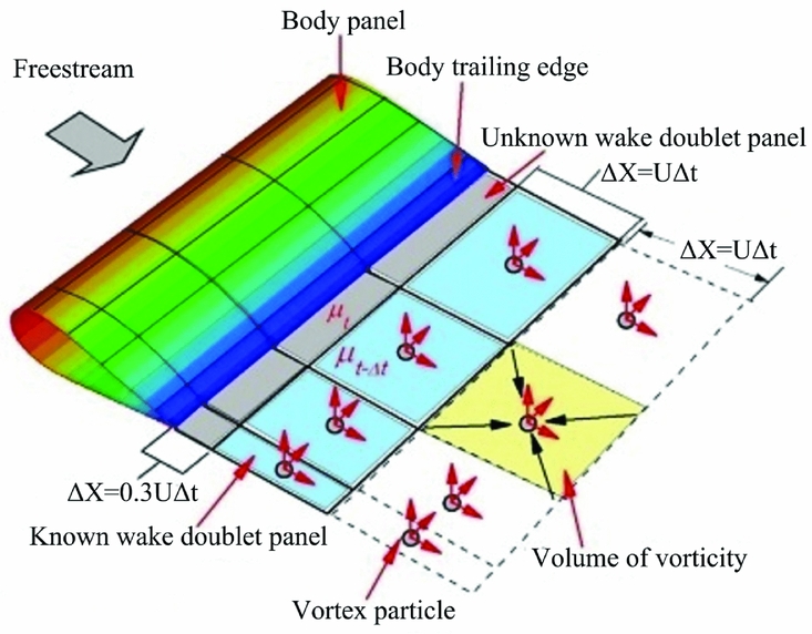
Figure 1. Conversion of constant strength wake doublet panels to vortex particles.
The relationship between doublet wake panels and vortex particles can be established by Hess's demonstration(Reference Hess22) as depicted in Equation (16), which indicates that the velocity at an arbitrary point in the flow domain caused by a doublet surface is equal to the sum of the velocities induced by both a vortex sheet of strength γ = n × ∇μ on Sw and a vortex filament of strength μ around the perimeter of the given panel Cw .
 $$\begin{equation}
{u_\mu }(x) = \frac{1}{{4\pi }}\int_{{C_W}} {\mu \frac{{d{\bm l} \times {\bm r}}}{{{r^3}}}} ds - \frac{1}{{4\pi }}\int_{{s_w}} {{\bm \gamma } \times \frac{{\bm r}}{{{r^3}}}} ds
\end{equation}$$
$$\begin{equation}
{u_\mu }(x) = \frac{1}{{4\pi }}\int_{{C_W}} {\mu \frac{{d{\bm l} \times {\bm r}}}{{{r^3}}}} ds - \frac{1}{{4\pi }}\int_{{s_w}} {{\bm \gamma } \times \frac{{\bm r}}{{{r^3}}}} ds
\end{equation}$$
2.4 Particle influence on panels
It is obvious that the vortex-particle wake has important influence on the body panel. When the vortex particles are included, their influences can be accounted for by adding the induced velocities of all wake particles into the Neumann boundary condition. Therefore, the new source strength(Reference Calabretta23) of each panel can be rewritten as
 $$\begin{equation}
\sigma = - {\bm n} \cdot \left( {{{\bm V}_0} + \sum\limits_{q = 1}^N {{\bm u}_{{\rm{ind}}}^q} } \right)
\end{equation}$$
$$\begin{equation}
\sigma = - {\bm n} \cdot \left( {{{\bm V}_0} + \sum\limits_{q = 1}^N {{\bm u}_{{\rm{ind}}}^q} } \right)
\end{equation}$$
where
 ${\bm u}_{{\rm{ind}}}^q$
is the induced velocity of the particle q, it can be obtained through the Biot-Savart law.
${\bm u}_{{\rm{ind}}}^q$
is the induced velocity of the particle q, it can be obtained through the Biot-Savart law.
2.5 Validation
In order to validate the proposed panel/viscous vortex particle hybrid method, two wind tunnel models with experimental data are used to make comparisons with our calculation results. The first model, i.e. a low Reynolds number aerofoil Eppler 387, is used to validate the accuracy of the wing drag because the viscosity effect of the air is considered in the hybrid method. The second one is a two-blade rotor, which is utilised for the purpose of demonstrating the accuracy of the hybrid method for the rotating machinery. For the panel method, panel density has an important effect on the calculated results, and the sensitivity of this method to panel density has been investigated by many researchers(Reference Richason, Katz and Ashby24-Reference Smith and Ross27). In this section, the Eppler 387 aerofoil is modelled by 40 chordwise panels and the rotor is panelled with 30 chordwise panel rows and 20 spanwise panel columns.
2.5.1 Example 1: E387 aerofoil
Computational results for the E387 aerofoil are described in Fig. 2 and compared with experimental data(Reference Robert, Walker and Milard28) and CFD results. The Reynolds number based on the aerofoil chord is Re = 4.6 × 10⁵ and the Mach number is 0.13. CFD simulations are conducted using the commercial software ANSYS Fluent. The RANS solver is used for all computations. The first grid node near the wall is placed at y+< 1. Considering the important effect of the turbulence model on the numerical simulation result, the Spalart-Allmaras(Reference Rahman, Agarwal and Lampinen29) (SA) and Menter's k-ω SST(Reference Menter30) turbulence models as well as the k-kL -ω transition model(Reference Walters and Leylek31) are selected to analyse the turbulence model sensitivity.
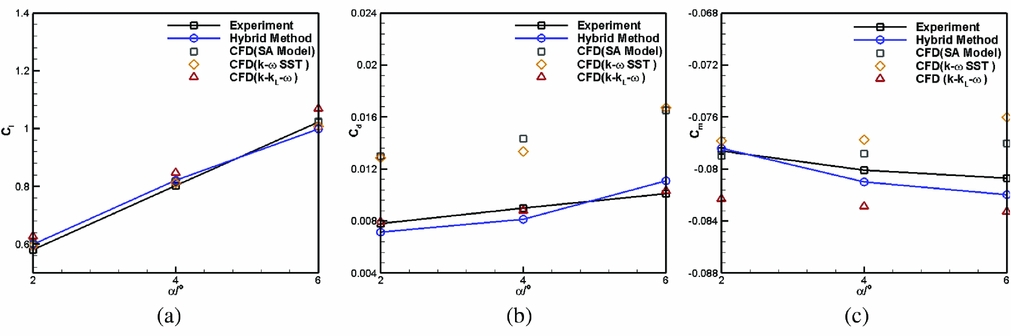
Figure 2. Aerodynamic forces comparison of E387 aerofoil. (a) Lift coefficient. (b) Drag coefficient. (c) Moment coefficient.
The results presented in Fig. 2 indicate that the lift coefficients obtained with both the turbulence model and the transition model show good agreements with experimental data. However, the k-kL -ω transition model is more accurate than the turbulence models in predicting the drag and pitching moment of the wing for a low Reynolds number flow. The difference between the turbulence model and the transition model is that the transition model has the ability of correctly describing the transition from a laminar flow to a turbulent flow which often occurs in the practical situation. Owing to the difference above, the lift of the aerofoil solved by the turbulence model is a little smaller than that for the transition model but the drag, especially the skin-friction drag, is overestimated. Because of these discrepancies in lift and drag of the aerofoil, the pitching moment calculated by the turbulence model is less accurate than that for the transition mode, especially when the free-stream angle is increased. For all these reasons, the k-kL -ω transition model will be used for all the subsequent CFD calculations in this paper.
2.5.2 Example 2: helicopter rotor
In this example, we demonstrate the accuracy of the hybrid method by rotating a pair of high aspect ratio and untwisted wings (see Fig. 3) in hovering condition. This two-blade rotor(Reference Caradonna and Tung32) uses a NACA0012 profile and has a collective pitch angle of a = 8°. The aspect ratio of a single blade is 6 and the rotational speed in this experiment is 1250 r/min.

Figure 3. Panel model of a two-blade rotor.
In Table 1, the rotor thrust coefficient obtained from the current method is also compared with the experimental data and CFD results. There is only a small difference between them, showing a good accuracy of this hybrid method.
Table 1 Force measurements comparison

The chordwise pressure distribution for two blade sections is given in Fig. 4. It can be seen that the calculation results of the panel/vortex-particle hybrid method are close to the CFD results and the experimental data(Reference Caradonna and Tung32), which were measured in the U.S. Army Aeromechanics Laboratory. The accuracy of the hybrid method is desirable for the purpose of fast prediction of the overall aerodynamic force.

Figure 4. Chordwise pressure distribution at different radial sections on one rotor blade. (a) r/R = 0.5. (b) r/R = 0.8.
3. RESULTS AND DISCUSSIONS
3.1 The tractor propeller configuration
In this section, the wing's aerodynamic behaviours affected by the propeller for a tractor propeller configuration (Fig. 5) are investigated using the panel/vortex-particle hybrid method. The rectangular wing has an aspect ratio of 2 and is modelled by 40 chordwise and 20 spanwise panels totaling 800 panels. The Reynolds number based on the root chord of the wing is Re = 4.88 × 10⁵ at the flight altitude of 20 km. The free-stream velocity direction points in the positive x axis and the angle-of-attack is selected as 2°. The propeller we designed has a rotational speed of 1500 r/min and a clockwise rotational direction observed from the downstream position. It is panelled with 30 chordwise panel rows and 20 spanwise panel columns.
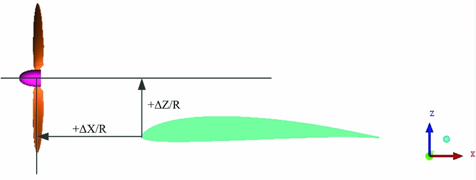
Figure 5. Single tractor propeller-wing configuration.
A comparison of aerodynamic coefficients between the CFD method and the hybrid method is presented in Table 2. For the CFD method, two different mesh densities, i.e. a coarse grid of 5.2 million cells and a fine grid of 9.5 million cells, have been tested to see their influence on the calculation results. As can be seen, there is small difference in the wing's lift, pitching moment and the propeller thrust between these two methods. Considering the results solved by two different mesh densities for the CFD method are very close to each other, all the subsequent calculations for the CFD method are conducted with the 5.2 million cells grid.
Table 2 Comparison of aerodynamic coefficients

Compared with the drag coefficient provided by the CFD method, there is a relatively larger drag error for the hybrid method even if the drag error can be reduced to be 6.25% with a fine mesh grid. In future work, it is necessary for us to study some relevant calculation parameters’ effect (such as the panelling density) in detail and update the unreasonable parameter used in the hybrid method for the purpose of further reducing the calculation error, especially the drag error, between the hybrid method and the experiment or the CFD method.
3.1.1 Effects of the streamwise position
Figure 6 presents the effects of propeller chordwise and vertical installed positions on the wing's aerodynamic performance. In this figure, R is the propeller radius, ΔX/R and ΔZ/R are the dimensionless horizontal and vertical distances between the propeller rotation centre and the leading edge of the wing, respectively. A positive value of ΔZ/R means the propeller is installed at a high vertical position relative to the wing.

Figure 6. Effect of propeller chordwise position on lift and drag coefficients of the wing. (a) Lift coefficient. (b) Drag coefficient.
It is clearly shown that the propeller slipstream leads to the increases of the lift and the drag on the wing. For example, when the propeller is installed at the position (ΔX/R = 0.5, ΔZ/R = 0.5), there is only a 2.01% increment in the lift coefficient but a 13.3% augmentation in the drag coefficient, as a result, the lift-to-drag ratio is decreased by 10%. In addition, it is apparent that a far horizontal position and a high vertical installed position of the propeller relative to the wing's leading edge are favourable for increasing the wing's lift and decreasing the drag.
The main reason of the augmentations of the wing's lift and drag can be attributed to the increased total and dynamic pressures of the propeller slipstream because of the propeller rotation. The increased dynamic pressure causes an acceleration of the axial velocity after the propeller, as a result, the propeller slipstream contracts its stream tube according to the principle of mass conservation. When the slipstream encounters the wing located at the downstream position, the contraction of the stream tube is strengthened and a more lift augmentation is obtained.
Besides the acceleration of the axial velocity, a tangential velocity component is also produced by the propeller rotation. The tangential velocities distributed at two sides of the propeller axis have equal magnitudes but opposite directions. For a traditional tractor propeller configuration, this tangential velocity distribution induces both upwash and downwash regions on the wing surface. In the upwash region, the effective local angle-of-attack is increased, which generates an augmentation of the section lift of the wing. In the downwash region, however, the down-going propeller blade leads to the decrease of the effective local angle-of-attack, so the section lift of the corresponding wing area is reduced.
Because of the upwash and downwash regions generated by the propeller, the distribution of the spanwise load of the wing has phenomena of peak and trough at two sides of the propeller axis as illustrated in Fig. 7. It can be clearly seen that the range of the wing affected by the propeller slipstream is almost equal to the propeller diameter. The rotational direction and installed position of the propeller will determine the locations of the load peak as well as trough and dominate the final shape of the spanwise load distribution of the wing.
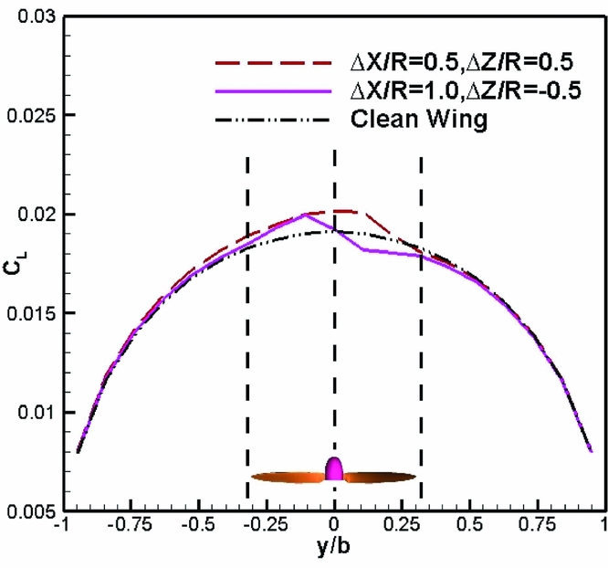
Figure 7. Spanwise lift distribution of the wing with the influence of a single propeller.
For a subsonic flow, there is a mutual interaction between the propeller and the wing. The propeller slipstream, significantly affecting the wing's aerodynamic behaviour, also conversely affects its own performance. Figure 8 shows the changes of propeller thrust coefficient versus five chordwise positions and three vertical positions of the propeller. CFD simulation results are also given for the purpose of comparisons. The maximum difference between the current approach and the CFD method is only 3.5%, which shows a good accuracy of the hybrid method used in this paper.
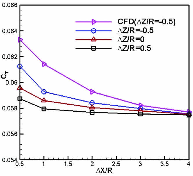
Figure 8. Effect of streamwise locations of the single propeller on propeller thrust coefficient.
It indicates that an increased chordwise distance leads to a decreasing propeller thrust coefficient and the propeller thrust falls slowly when ΔX/R > 2. Because the wing is located downstream from the propeller, it decreases the velocity of the propeller slipstream but increases the slipstream's static pressure behind the propeller disk. This is so-called the wing’s aerodynamic interference on the propeller and it is helpful to augment the propeller thrust. However, this beneficial interference will be quickly weakened as the chordwise distance is enlarged, as a result, the propeller thrust at a larger ΔX/R is smaller than that at a smaller ΔX/R. In addition, Fig. 8 also indicates that a lower vertical propeller position is favourable for the propeller thrust.
3.1.2 Effects of the spanwise position
The influence of the propeller spanwise position on the wing is investigated in this section. In Fig. 9, the results are depicted corresponding to a propeller chordwise position ΔX/R = 1.0 and a vertical position ΔZ/R = −0.5.
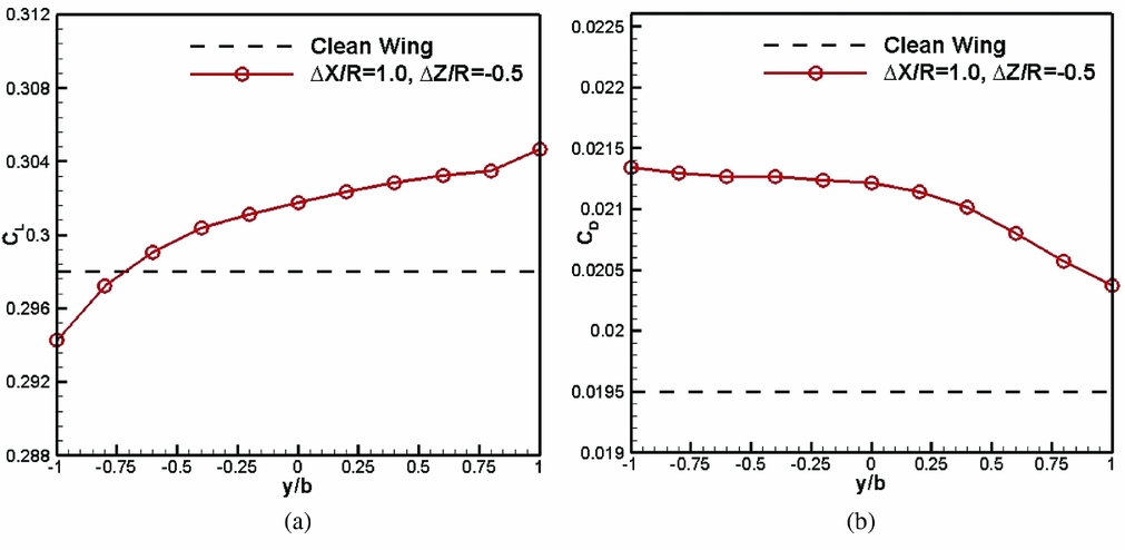
Figure 9. Effect of propeller spanwise positions on the wing. (a) Lift coefficient. (b) Drag coefficient.
Compared with the clean wing, the benefits, i.e., a lift increase and a drag decrease, can be obtained apparently when the propeller is moved from the left tip (y/b = –1) to the right tip (y/b = 1) of the wing. The main reason for this result is the coaction of the upwash and downwash effects of the propeller on the wing. As described above, the propeller rotates clockwise observed from a downstream position. When it is mounted at the left tip of the wing, only the propeller downwash directly washes the wing. This downwash effect leads to the decreased effective angle-of-attack, as a result, less lift but more induced drag are generated in this case. On the contrary, when the propeller is installed at the right wing tip, it is the propeller upwash that directly influences the wing. The increased effective angle-of-attack creates a bigger lift and a smaller induced drag.
3.2 The over-the-wing propeller configuration with a single propeller effect
The calculation results described in Fig. 6 indicates that the lift increment and the drag decrement can be obtained when the propeller is moved upward. This is because the high vertical installed propeller position makes the propeller slipstream mainly affect the upper surface of the wing and the velocity of the flow around the wing's upper surface is accelerated by the propeller rotation.
Inspired by this result, a new propeller-wing configuration (see Fig. 10), i.e. an over-the-wing propeller (OTWP) configuration is investigated in this section. In this configuration, the propeller is located over the wing in order to make the entire propeller slipstream beneficially influence the wing's upper surface.
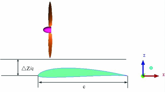
Figure 10. Over-the-wing propeller (OTWP) configuration.
In Fig. 11, the aerodynamic behaviour of the wing versus the propeller chordwise position is depicted for three clearance values of ΔZ/c = 0.187, 0.287, 0.387.
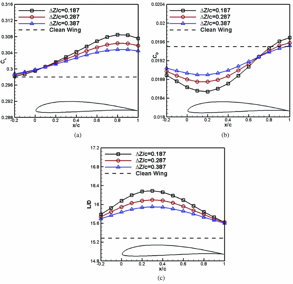
Figure 11. Effect of propeller chordwise positions on the OTWP configuration with a single propeller. (a) Lift coefficient. (b) Drag coefficient. (c) Lift-to-drag ratio.
Compared with the results presented in Fig. 6, the OTWP arrangement has favourable effects on both the lift and the drag of the wing, i.e. significant lift increment and drag reduction can be obtained. The maximum of the lift gain corresponds to the propeller chordwise position of x/c = 0.8, the maximal drag reduction occurs at x/c = 0.2, but the maximum lift-to-drag ratio is found at x/c = 0.3.
For the OTWP configuration, there is no propeller slipstream that directly washes the wing so that the acceleration of the axial free-stream velocity plays a more important role than the upwash and downwash effects of the propeller in changing the wing's aerodynamic performance. Because of the propeller's rotation, the dynamic pressure of the uniform free-stream in front of the propeller is increased, as a result, a region with a smaller static pressure on the upper surface of the wing is created, which is responsible for the lift augmentation when the propeller is moved backward.
The reduction in the drag of the wing is the key aerodynamic feature of this configuration and it benefits from two parts: a suction effect and a pushing effect. For the flow in front of the propeller disc, the velocity is accelerated by the propeller so that the leading-edge suction force of the wing is enhanced and it creates a suction effect that slightly pulls the wing forward. For the flow behind the propeller disc, however, both the total and static pressures are increased and a pushing effect is generated. This effect generates a pushing force acting on the rear segment of the wing to further decrease the wing drag.
3.3 The OTWP configuration with double propellers effect
The results of the OTWP configuration described above have proved its considerable advantages to improve the aerodynamic performance of the wing. In order to exploit more benefits in this arrangement, double propellers are utilised to further investigate this configuration. The clearance between the propeller tip and the wing's leading edge is selected as ΔZ/c = 0.187 and the rotational speed of these two propellers is still 1500 r/min.
As for double propellers, their rotational direction is an important factor affecting the performance of the wing. The OTWP configuration with double propellers is shown in Fig. 12 with a rear view. The plus sign represents the positive rotational direction of the propeller, i.e. the clockwise rotational direction. If both of these two propellers rotate with positive directions, we denote them as (P1+, P2+). In this section, two kinds of propeller rotational directions, i.e. (P1+, P2+) and (P1+, P2-), are selected for the simulations.

Figure 12. OTWP configuration with double propellers.
3.3.1 Streamwise position effect
The effect of the double propellers’ streamwise position on the wing is presented in Fig. 13. As can be seen, the position where the maximum of the wing lift can be obtained is still at x/c = 0.8 (Fig. 13(a)) and the maximum of the lift-to-drag ratio also occurs at x/c = 0.3 (Fig. 13(c)). It should be mentioned that the spanwise distance between the double propellers is selected as ΔY/R = 2.5 and kept as a constant value (ΔY/R is the dimensionless spanwise distance in Fig. 12) in order to make sure that there is only one propeller parameter that is investigated.

Figure 13. Effect of the double propellers’ streamwise location on the OTWP configuration. (a) Lift coefficient. (b) Drag coefficient. (c) Lift-to-drag ratio.
Although the trends of these curves are as the same as that shown in Fig. 11, the magnitudes of the lift and the lift-to-drag ratio are apparently raised and the drag is further reduced compared with the OTWP configuration with a single propeller. This phenomenon can be explained by the enhanced suction effect and pushing effect on the wing's upper surface caused by two propellers. The detailed calculation results corresponding to the propeller chordwise position x/c = 0.3 are depicted in Table 3. It is evident that the slipstream of the double propellers is more favourable than that of the single one for the performance of the wing. The increments of the lift, lift-to-drag ratio and the decrement of the drag can be achieved by 3.99%, 17.60% and 11.54%, respectively, relative to the clean wing.
Table 3 Comparison of OTWP configuration results with single-propeller and double-propellers

3.3.2 Spanwise position effect
The spanwise distance between the two propellers is also important to affect the wing's aerodynamic behaviour. In this section, a range of ΔY/R = 2.5 to 6.0 is selected to perform the analysis. It should be explained that the value of ΔY/R = 6 corresponds to the location where these two propellers are mounted at two tips of the wing. Similarly, in order to ensure that there is only one influencing parameter, the double propellers’ streamwise position is selected as x/c = 0.3. The results in Fig. 14 indicate that an increasing spanwise distance induces a decrement in the wing lift but an increment in the wing drag, and hence a decrease of the lift-to-drag ratio. The reason for this unfavourable result is that a larger spanwise distance gradually abates the beneficial interactions between the double propellers and the wing.

Figure 14. Effect of spanwise distance for the OTWP configuration with double propellers. (a) Lift coefficient. (b) Drag coefficient. (c) Lift-to-drag ratio.
In order to demonstrate the feature of the pressure distribution of the OTWP configuration, the spanwise load distributions at the positions ΔY/R = 2.5 and ΔY/R = 6.0 are plotted in Fig. 15. These curves indicate that the upwash and downwash regions occurring in a traditional tractor propeller arrangement vanish in the OTWP configuration. This is because there is no propeller slipstream directly washing the wing when the propeller is located over the wing and hence the effective angle-of-attack at the leading edge of the wing does not change significantly. Due to the disappearances of the upwash and downwash effects, the acceleration of the free-stream velocity becomes the major factor of improving the wing's aerodyanmic performance, which has been proved by the results in Fig. 15.

Figure 15. Spanwise lift distribution for the OTWP configuration with double propellers.
4. CONCLUSIONS
The present paper investigates the influence of the propeller location parameter on the wing aerodynamics using a panel/viscous vortex particle hybrid method. This method considering the air viscosity effects can accurately predict the wing's aerodynamic behaviour influenced by the propeller. Although it can't capture the detailed flow field characteristics, its computational cost is much lower than that of the CFD method and it can be used to rapidly obtain the wing overall aerodynamics to perform conceptual design studies.
For a traditional tractor-propeller configuration, the wing is immersed in the propeller slipstream and the accelerated free-stream velocity and the tangential velocity are induced by the propeller. Affected by these two effects, both the wing lift and drag are increased compared with that of the clean wing. When the propeller is located at a high vertical position, the wing aerodynamic performance can be improved slightly.
The over-the-wing propeller (OTWP) configuration has advantages in increasing the wing lift and reducing the drag compared to the traditional propeller-wing layout. A small clearance between the propeller tip and the wing and a large propeller number are favourable to further improve the wing performance. For the double-propeller case, the maximum increment of the lift-to-drag ratio can be achieved by 17.6% when the propeller is located at 30% of the wing chord. Maybe the OTWP configuration is suitable for the distributed propulsion aircraft from the perspective of aerodynamics. Therefore, future work shall focus on the detailed investigation of the effects of the distributed propeller's parameters, including the propeller's number, the spanwise distance, and the rotational direction and speed, on the wing's aerodynamic performance in order to exploit more aerodynamic potentials of this new configuration.


