3.1 Overview of the flow

In figure 3 instantaneous fields of the vorticity magnitude are shown on the meridian planes $a$ , $b$ and $c2$ defined in figure 4(a). The effectiveness of the numerical trip wire is evident, as the boundary layer becomes turbulent immediately downstream of the tripping location. In computations where the disturbance was switched off (not shown here), the boundary layer transitioned only directly downstream of the sail, which caused early separation at the stern and a consequent displacement of the wake. When the trip wire is used no separation occurs along the stern. Figure 3(a) highlights that the main areas of turbulent activity, in addition to the boundary layer, are the wake of the fins and the sail. The wake of the sail affects the turbulent boundary layer on the upper side of the hull. The turbulent structures generated in the wake of the sail, however, are not the main feature of the flow in the near and the intermediate wake of the overall body, which is dominated by the structures generated at the trailing edge of the fins and in the thick boundary layer developing along the stern.

Figure 3. Instantaneous fields of the non-dimensional vorticity ${\it\omega}D/U_{\infty }$ , where $U_{\infty }$ represents the free-stream velocity: plane $a$ (a), plane $b$ (b) and plane $c2$ (c). For the orientation of the meridian planes refer to figure 4.

Figure 4. (a) Projection of the meridian planes $a$ , $b$ , $c1$ and $c2$ on the cross-stream plane $yz$ . (b) Lateral view of the DSub model representing the position of the reference frame.

In the horizontal plane shown in figure 3(b) the general flow properties are similar. On the plane $c2$ shown in figure 3(c) it is evident that the influence of all appendages (sail and fins) is much weaker than in the previous planes. The vorticity field displays two maxima away from the axis. As we will discuss below, these are due to the boundary layer developing along the stern: the adverse pressure gradient at the rear of the DSub causes a displacement of the peaks of turbulent activity away from the surface of the stern and thus away from the axis of the wake. A more detailed view of the flow along the stern is shown in figure 5, where instantaneous vorticity on cross-sections is shown. It is clear that the flow upstream of the appendages on the stern is mainly affected by the turbulent structures in the boundary layer developing along the stern and less by the sail wake. On the section A–A the highest values of instantaneous vorticity are associated with the flow from the tip of the fins, where the strongest unsteady activity is observed. Looking at the downstream evolution along the stern, one can see that the vorticity due to the flow from the tip of the fins fades out more quickly than that originated from the boundary layer. This is also one of the main features of the wake and will be discussed in detail in the next section. We should also note that the instantaneous vorticity magnitude above is simply used to provide a qualitative overview of the main flow features. Given the dependence of the vorticity fields on the SGS modelling (see, for example, Galperin Reference Galperin1993) we do not report vorticity statistics in the present work.

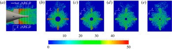
Figure 5. Instantaneous magnitude of the non-dimensional vorticity ${\it\omega}D/U_{\infty }$ in the near wake of the fins. In (a) a detail of the field in figure 3(a) is represented, showing the location of the cross-sections A–A (b), B–B (c), C–C (d) and D–D (e).

Figure 6. (a) Time-averaged pressure coefficient; (b) time-averaged skin-friction coefficient and acceleration parameter $K$ at different locations along the DSub surface. Present results: —— plane $a$ on the side of the negative $y$ axis (location 1); – – – plane $a$ on the side of the positive $y$ axis (location 2); — ⋅ — average between planes $c1$ and $c2$ on the side of the negative $y$ axis (location 3). Experimental results: ▫ Huang et al. (Reference Huang, Liu, Groves, Forlini, Blanton and Gowing1994) at $\mathit{Re}_{L}=12\times 10^{6}$ ;  $\bullet$  Jiménez et al. (Reference Jiménez, Hultmark and Smits2010a ) at $\mathit{Re}_{L}=1.1\times 10^{6}$ . ▵ RANS computation by Gorski, Coleman & Haussling (Reference Gorski, Coleman and Haussling1990) on the unappended DSub at $\mathit{Re}_{L}=12\times 10^{6}$ . — — —  $C_{f}$ slope for a zero-pressure-gradient turbulent boundary layer on a flat plate (Schlichting Reference Schlichting1968). In (b) the acceleration parameter $K$ is also reported as $\bullet$ . The $C_{f}$ distribution by Huang et al. (Reference Huang, Liu, Groves, Forlini, Blanton and Gowing1994) was rescaled, based on the Reynolds numbers ratio.

3.2 Statistics along the surface of the body

In this section the evolution of the boundary layer along the hull is discussed. As the symmetry around the axis is lost due to the presence of the appendages, the evolution of the boundary layers is different on different azimuthal planes. In figure 6 the pressure, $C_{p}$ , and skin-friction, $C_{f}$ , coefficients:

(3.1a,b ) $$\begin{eqnarray}C_{p}=\frac{p-p_{\infty }}{\frac{1}{2}{\it\rho}U_{\infty }^{2}},\quad C_{f}=\frac{{\it\tau}_{w}}{\frac{1}{2}{\it\rho}U_{\infty }^{2}},\end{eqnarray}$$

are shown at different planes. Note that $p_{\infty }$ is the free-stream pressure at the inflow plane, ${\it\rho}$ the density of the fluid, and ${\it\tau}_{w}$ the wall stress. The variation along the plane $a$ , for both negative (location 1) and positive (location 2) $y$ coordinates, and the average along planes $c1$ and $c2$ (location 3) are shown (see figure 4 for the definition of the different planes). The experimental results by Huang et al. (Reference Huang, Liu, Groves, Forlini, Blanton and Gowing1994) and Jiménez et al. (Reference Jiménez, Hultmark and Smits2010a ) as well as the computations by Gorski et al. (Reference Gorski, Coleman and Haussling1990) are included. In both experiments the geometry has no stern appendages, while the Reynolds numbers are $12\times 10^{6}$ and $1.1\times 10^{6}$ , respectively. The $C_{p}$ distribution by Gorski et al. (Reference Gorski, Coleman and Haussling1990) comes from a RANS simulation of the flow around the unappended DSub model at Reynolds number equal to $12\times 10^{6}$ . A body-fitted grid was utilized in that case. The reference measurements have been carried out in areas away from the direct influence of the support and are, therefore, comparable to the numerical results at location 2, where the effect of the sail is minimal. The present results are in good agreement with both the measurements by Huang et al. (Reference Huang, Liu, Groves, Forlini, Blanton and Gowing1994) and the computations by Gorski et al. (Reference Gorski, Coleman and Haussling1990). It is interesting to note that the RANS computations by Gorski et al. (Reference Gorski, Coleman and Haussling1990) reproduce accurately the distribution of the pressure coefficient, indicating that in the absence of separation phenomena and secondary flows RANS captures the displacement caused by the boundary layers fairly well. The same computations, however, also point to the limitations of RANS to accurately predict important quantities, such as the skin-friction coefficient, $C_{f}$ : their results indicate that doubling the grid resolution along the radial and axial directions resulted in an increase of about 50 % for $C_{f}$ . The same trends have been observed in the study by Alin et al. (Reference Alin, Bensow, Fureby, Huuva and Svennberg2010), who simulated both unappended and appended DSub at $\mathit{Re}_{L}=12\times 10^{6}$ using RANS, DES and wall-modelled LES. They compared their $C_{p}$ and $C_{f}$ distributions to the experiments by Huang et al. (Reference Huang, Liu, Groves, Forlini, Blanton and Gowing1994), and while $C_{p}$ was predicted accurately by all models, $C_{f}$ was underestimated in all cases. The RANS results had the most significant deviations from the experiments, especially in the stern region, where strong adverse pressure gradients are generated by the hull geometry. Similar results were reported by Bhushan et al. (Reference Bhushan, Alam and Walters2013), who simulated the appended DSub at $\mathit{Re}_{L}=12\times 10^{6}$ by URANS, DES and hybrid RANS/implicit LES: the $C_{p}$ distribution was predicted equally well by all methods, while $C_{f}$ was best captured by the hybrid RANS/LES methodology.

In our computations the overall evolution of $C_{p}$ agrees with the results by Jiménez et al. (Reference Jiménez, Hultmark and Smits2010a ), although there is an offset. Jiménez et al. (Reference Jiménez, Hultmark and Smits2010a ) suggested that this offset is likely caused by a different value of the reference pressure. They adopted as $p_{\infty }$ the pressure at $14.75D$ upstream of the model nose, while Huang et al. (Reference Huang, Liu, Groves, Forlini, Blanton and Gowing1994) considered a location above the model at $x/D\approx 7.3$ , that is $1.3D$ upstream of its tail; in the present case the reference pressure was taken at the inflow, which is at $2.6D$ from the nose. Our numerical experiments on coarser grids indicate that the location of the inflow plane relative to the nose has a small effect on $C_{p}$ , suggesting that this may not be the reason for the disagreement, which is likely due to blockage. Jiménez et al. (Reference Jiménez, Hultmark and Smits2010a ) reported a blockage in their closed-loop wind tunnel, due to both SUBOFF body and support, equal to 5.7 %, while in our computational domain it was only 1.4 %. Furthermore, the wake of the support is obviously much wider than that of the actual sail, considered in this numerical study. Note that the measurements by Jiménez et al. (Reference Jiménez, Hultmark and Smits2010a ) shown in figure 6(a) are from the side opposite to the support.

The evolution of the skin-friction coefficient at the same locations is shown in figure 6(b), together with the acceleration parameter $K=({\it\nu}/U_{t}^{2})(\text{d}U_{t}/\text{d}s)$ at location 3 ( $U_{t}$ is the local tangential velocity at the edge of the boundary layer and $s$ the coordinate along the local streamline). In this case the slope of $C_{f}$ for a zero-pressure-gradient turbulent boundary layer along a flat plate (ZPGFPBL) has been added for reference. The evolution of $C_{f}$ at all positions is very similar, up to the edge between the bow and the mid-body ( $x/L\approx 0.2$ ). Due to the curvature of the body a peak is present there, associated with the acceleration of the flow, as indicated by $K$ . It is likely that the blockage by the sail causes higher values of $C_{f}$ at the azimuthal location 3 (closer to the sail) than at the location 2, on the opposite side. Also note that at position 1, immediately downstream of the sail, the value of $C_{f}$ is even larger, compared with the other profiles, due to the junction flows, which bring high momentum fluid towards the root of the sail. Downstream of the sail the rate of change of $C_{f}$ is very close to that of a ZPGFPBL, especially on the side away from the sail, which is consistent with the nearly zero values of the acceleration parameter in that region. At the beginning of the stern ( $x/L\approx 0.75$ ) the profiles of $C_{f}$ collapse again, which suggests that the influence of the sail wake becomes negligible, at least on the development of the boundary layer along the stern, where the flow decelerates significantly, as indicated by $K$ . Downstream of the fins the skin friction is higher in their wake than in the planes away due to the junction flows. Both the pressure and the skin-friction coefficients show that near the tail the flow experiences a slight acceleration and then a deceleration due the change of curvature of the stern.

The experiments by Jiménez et al. (Reference Jiménez, Hultmark and Smits2010a ) do not report $C_{f}$ distributions to compare directly with the present LES. In figure 6(b), however, we included the results by Huang et al. (Reference Huang, Liu, Groves, Forlini, Blanton and Gowing1994) at a much higher Reynolds number ( $\mathit{Re}_{L}=12\times 10^{6}$ ), rescaling them using the Reynolds numbers ratio. Note that these are measurements on a bare hull configuration. The comparison with the present results is good especially in the area downstream of the sail. Upstream of the sail the predicted $C_{f}$ is higher than the experiment probably due to the acceleration caused by the sail. The same trend has been reported in the computations by Alin et al. (Reference Alin, Bensow, Fureby, Huuva and Svennberg2010).

Figure 7. Time-averaged (a) momentum thickness Reynolds number, $\mathit{Re}_{{\it\theta}}$ , and (b) shape factor, $H$ , along the DSub surface. Present results: – – – plane $a$ on the side of the positive $y$ axis; — ⋅ — average between planes $c1$ and $c2$ on the side of the negative $y$ axis. — — — ZPGFPBL (Schlichting Reference Schlichting1968).

In figure 7 the evolution of the Reynolds number based on the momentum thickness, $\mathit{Re}_{{\it\theta}}={\it\theta}U_{\infty }/{\it\nu}$ , and the shape factor, $H={\it\delta}_{1}/{\it\theta}$ , where ${\it\delta}_{1}$ is the displacement thickness and ${\it\theta}$ the momentum thickness, are plotted downstream of the trip for positions 2 and 3 (position 1 is not shown, since it is strongly affected by the wake of the sail). The corresponding slope for a ZPGFPBL has been added for comparison. Along the mid-body the slope of $\mathit{Re}_{{\it\theta}}$ , as well as $H$ , compares fairly well with that of a ZPGFPBL, indicating that in this region the boundary layer is almost in equilibrium. Outside this region deviations from this behaviour can be observed. $\mathit{Re}_{{\it\theta}}$ , for example, shows an increased slope just downstream of the edge between the bow and the mid-body ( $x/L\approx 0.2$ ), due to a mild adverse pressure gradient (see figure 6 a). The slope decreases along the cylindrical mid-body, because of the gradual reduction of the pressure gradient. This trend becomes more obvious between $x/L=0.7$ and $x/L=0.75$ , due to the local acceleration of the flow (the thickness of the boundary layer is decreasing). Along the stern the boundary layer grows significantly. The agreement between the numerical profiles is very close up to the appendages on the stern ( $x/L=0.85$ ), which shows that the influence of the sail wake is limited.

Figure 8. Streamwise velocity fluctuations relative to the mean field on an ‘unrolled’ cylindrical slice of the computational grid at 10 wall-units from the surface of the mid-body. The coordinates along the spanwise and streamwise directions are provided in wall-units. The fluctuations are non-dimensionalized by the free-stream velocity, $U_{\infty }$ . Note that the origin of the streamwise axis is located at the tail of the stern. (a) Global view, where – – – and — ⋅ — represent the beginning and the end of the cylindrical mid-body; (b) detail, shown in (a) by a white box, at an azimuthal location $90^{\circ }$ away from the sail in the mean streamwise region of the mid-body.

Next we will take a closer look at the boundary layer in the mid-body area. Figure 8 shows a snapshot of the instantaneous streamwise velocity fluctuations on an unrolled cylindrical slice of the computational grid 10 wall-units away from the surface (the average $u_{{\it\tau}}$ in the range $0.3<x/L<0.6$ is used for all inner scaling). The coordinates along the azimuthal and axial directions are provided in wall-units. The presence of the typical streaks, associated with the quasi-streamwise vortices inside the boundary layer, is visible. It is also interesting that the sail does not affect significantly the streaks in its wake. In the detailed view (figure 8 b) the actual dimension of the streaks is shown and is in agreement with the values reported in the literature: their streamwise extent is in the order of 1000 wall-units and their spacing along the cross-stream direction is equivalent to few hundreds wall-units.

Figure 9. Statistics in wall-units in the turbulent boundary layer at the mean streamwise position of the DSub model: – – – along the positive $y$ axis (side away from the sail); —— along the negative $y$ axis (side downstream of the sail); ○ DNS on a ZPGFPBL by Spalart (Reference Spalart1988) at $\mathit{Re}_{{\it\theta}}=1410$ ; $\times$ measurements by DeGraaff & Eaton (Reference DeGraaff and Eaton2000) at $\mathit{Re}_{{\it\theta}}=1430$ . (a) Time-averaged streamwise velocity $u$ ; (b) root mean squares $u^{\prime }$ , $w^{\prime }$ and $v^{\prime }$ of the streamwise, spanwise and normal velocity components. Here $x_{n}^{+}$ is the local coordinate in wall-units along the direction normal to the wall.

In figure 9 velocity statistics inside the boundary layer are shown in inner coordinates for both the azimuthal location aligned with the sail and the opposite one. Both mean velocity profiles have a logarithmic region with a slope that is in agreement with that of the universal law for a ZPGFPBL; however, their intercept is smaller, maybe due to the presence of the upstream sail, affecting the distribution of the skin-friction coefficient and friction velocity along the surface of the DSub, which are higher than those for a ZPGFPBL. At the edge of the boundary layer ( $x_{n}^{+}\approx 1000$ ) a deviation between the profiles on the opposite sides is observed: on the side away from the sail the wake of the turbulent boundary layer is clearly distinguishable, while its formation is prevented by the wake of the sail on the other side. The velocity fluctuations (see figure 9 b) are slightly underestimated in comparison with the values in the literature (Spalart Reference Spalart1988; DeGraaff & Eaton Reference DeGraaff and Eaton2000), which is probably due to the higher values of friction velocity. Grid resolution could also affect this behaviour, but due to the large computational cost of the present simulation further grid refinement was prohibitively expensive. However, based on the evolution of the acceleration parameter reported in figure 6(b), a deviation of the statistics in the boundary layer from those of a ZPGFPBL can be expected: the present case displays a complex pattern of accelerations/decelerations, also dependent on the particular azimuthal position over the SUBOFF surface. At the same time the grid resolution over the cylindrical mid-body satisfies the requirements reported in the literature for wall-resolved LES (Georgiadis, Rizzetta & Fureby Reference Georgiadis, Rizzetta and Fureby2010).

3.3 Comparison with the experiments

In figure 10 the present results in the intermediate wake ( $6D$ from the tail) are compared with the hot wire measurements by Jiménez et al. (Reference Jiménez, Reynolds and Smits2010b ) at $z/D=0$ , corresponding to the plane through the sail. In figure 10(a) the comparison is provided in self-similar coordinates, which are the maximum velocity deficit, $u_{0}$ , the difference between the free-stream velocity and the minimum velocity in the wake, and the half-wake width, $l_{0}$ , the distance between the centre of the wake and the location where the momentum deficit is equal to $u_{0}/2$ . The similarity law for the mean streamwise velocity, proposed by Jiménez et al. (Reference Jiménez, Reynolds and Smits2010b ), is also included, where ${\it\eta}=y/l_{0}$ :

(3.2) $$\begin{eqnarray}f({\it\eta})=\exp (-0.525{\it\eta}^{2}-0.1375{\it\eta}^{4}-0.03{\it\eta}^{6}-0.002225{\it\eta}^{8}).\end{eqnarray}$$

In figure 10(a) for $-1<y/l_{0}<1$ the agreement between all profiles is very close. For $1<|y/l_{0}|<2$ on both sides the velocity defect in the numerical results is a little larger than in the experiments, probably due to the fact that this region is affected by wake of the fins. For $|y/l_{0}|>2$ the agreement with the experiments is again satisfactory on the side opposite to the sail. On the other side the numerical profile meets the theoretical curve much better than the experiments. This can be explained considering the larger velocity deficit produced in the wind tunnel by the wake of the support. In figure 10(b) the profiles of streamwise velocity are scaled by $U_{e}$ (velocity at the edge of the wake) and $D$ . The agreement with the experiment is good and the differences between measurements and computations can be justified: for negative $y$ coordinates the experimental profile does not recover the free-stream velocity, being affected by the large wake of the support. The blockage it generates is the likely reason of the higher velocities seen in the experimental profile for $y/D>-0.5$ . We verified that this effect is even more obvious in the offset planes, therefore at those locations we assumed more appropriate to compare between computations and experiments in self-similar coordinates: in figure 11 two offset planes are considered, for $z/D=0.125$ and $z/D=0.250$ , respectively. The agreement between simulation and experiments is again very good, and the largest discrepancies can be seen at $y/l_{0}\approx -2$ , due to the strong influence of the support in the experiments.

Figure 10. (a) Time-averaged streamwise velocity defects in similarity coordinates (the profiles are scaled by the maximum velocity defect, $u_{0}$ , and the half-wake width, $l_{0}$ ; $U_{e}$ is the velocity at the edge of the wake). (b) Time-averaged streamwise velocity profiles, scaled by $U_{e}$ and $D$ . Position at $x/D=6$ and $z/D=0$ . – – –, (3.2);  $\bullet$ , experiments by Jiménez et al. (Reference Jiménez, Reynolds and Smits2010b ); ——, LES.

Figure 11. Time-averaged streamwise velocity defects in similarity coordinates. Position at $x/D=6$ and (a) $z/D=0.125$ , (b) $z/D=0.250$ . – – –, (3.2);  $\bullet$ , experiments by Jiménez et al. (Reference Jiménez, Reynolds and Smits2010b ); ——, LES.

Figure 12. Time-averaged fields of the non-dimensional streamwise velocity $u/U_{\infty }$ : plane $a$ (a), plane $b$ (b) and average between planes $c1$ and $c2$ (c). For the position of the planes see figure 4(a).

A more global picture of the averaged velocity field is shown in figure 12, where the time-averaged streamwise velocity in the same planes considered in figure 3 is shown. Note that in figure 12(c) the average between the planes $c1$ and $c2$ (see figure 4) is plotted. The comparison among the three different fields further highlights the influence of the appendages on the stern to the mean flow. In the planes $a$ and  $b$ , especially in the vicinity of the DSub, an additional lack of momentum at the edge of the wake can be observed, relative to the field on the $c$ planes, due to the flow from the tip of the fins. As discussed above, this result has been verified also experimentally by Jiménez et al. (Reference Jiménez, Reynolds and Smits2010b ), who found that the main deviation from the wake of the unappended geometry is downstream of the tips of the stern appendages. Instead, figure 12(c) shows that in the planes away from the fins the near wake has a smaller diameter than that of the cylindrical mid-body, since the boundary layer on the stern stays attached, following the curvature of its surface. Further downstream the width of the wake on all three planes tends to converge, due to diffusion along the azimuthal direction. It is also shown in figure 12(a) that on the symmetry plane the overall wake is primarily affected by the momentum deficit caused by the fins and marginally by that associated with the sail, whose influence is mainly limited to the length of the cylindrical mid-body. It is also clear that the flow at the convex border between the cylindrical mid-body and the stern experiences an acceleration, with a consequent local decrease of the boundary layer thickness. This occurs also at the edge between the bow and the mid-body, although it is less evident in figure 12. The same behaviour has been observed in the experiments by Huang et al. (Reference Huang, Liu, Groves, Forlini, Blanton and Gowing1994) and Jiménez et al. (Reference Jiménez, Hultmark and Smits2010a ) and in the RANS simulations by Gorski et al. (Reference Gorski, Coleman and Haussling1990).

In figure 13 the profiles for the root mean square (r.m.s.) of the streamwise and radial velocity components and the shear stress in the $xy$ plane are shown at $x/D=6$ and $z/D=0$ , normalized by the velocity at the edge of the wake and the maximum hull diameter. These results are not plotted in similarity coordinates, because the Reynolds stresses are not self-similar at this distance from the stern. More details on this issue can be found in Jiménez et al. (Reference Jiménez, Hultmark and Smits2010a ,Reference Jiménez, Reynolds and Smits b ). The agreement between the experiments and the simulation is very good. The peaks at $y/D=\pm 0.2$ are accurately captured by the computation. Some deviations can be seen around $y/D=\pm 0.5$ and on the axis. On the side downstream of the sail at the edge of the wake the deviation of the experiments from the numerical results for $y/D<-0.5$ is due to the support: the effect of the sail wake in the simulation is much more localized than in the wind tunnel experiments and the r.m.s. go to 0, which implies a more symmetric profile. The radial velocity fluctuations (figure 13 b) are slightly over-predicted in comparison with the experiment near the axis ( $-0.2<y/D<0.2$ ). The wake of the appendages on the stern also causes higher fluctuations ( $0.4<|y/D|<0.6$ ). The bimodal distribution and the location of the maxima away from the axis of the wake are captured accurately.

Figure 13. R.m.s. of the velocity components along $x$ (a) and $y$ (b), and the shear stress in the $xy$ plane (c). Profiles at $6D$ from the tail of the stern at $z/D=0$ (plane through the sail). $\bullet$ , experiments by Jiménez et al. (Reference Jiménez, Reynolds and Smits2010b ); ——, LES.

The comparison on the shear stress is shown in figure 13(c); it is consistent with the ones for the r.m.s. of $u$ and $v$ . The experiments and the computation agree on the presence of 2 maxima away from the axis and on their location, although the numerical values are slightly higher. This behaviour is in line with the observations in the experiments by Jiménez et al. (Reference Jiménez, Hultmark and Smits2010a ,Reference Jiménez, Reynolds and Smits b ), who found that for the unappended geometry the semi-infinite sail had a destructive influence on the shear stress $u^{\prime }v^{\prime }$ , while the interaction of the wake of the support with that of the fins caused increased shear stresses for negative $y$ coordinates downstream of the appended DSub.

Figure 14. Fields of $k/U_{\infty }^{2}$ in the wake up to $9D$ from the stern tail: (a) plane $a$ ; (b) plane $b$ ; (c) average between planes $c1$ and $c2$ . See figure 4 for the location of the planes. The position of the upstream sail is indicated by a white arrow. Here ${\it\alpha}$ and ${\it\beta}$ are the regions of high turbulent kinetic energy associated respectively with the wake of the fins and the thick boundary layer shed from the stern surface.

3.4 Bimodal behaviour of the wake and effect of the fins

The results in the intermediate wake by Jiménez et al. (Reference Jiménez, Hultmark and Smits2010a ,Reference Jiménez, Reynolds and Smits b ), as well as the present simulation, show a bimodal behaviour for the normal stresses. Jiménez et al. (Reference Jiménez, Hultmark and Smits2010a ,Reference Jiménez, Reynolds and Smits b ) attributed it to the thick boundary layer developing along the stern of the DSub model. This is consistent with observations in earlier experiments by Patel, Nakayama & Damian (Reference Patel, Nakayama and Damian1974) and Merz, Yi & Przirembel (Reference Merz, Yi and Przirembel1986). In figure 14 the averaged turbulent kinetic energy, $k$ , is shown at three different meridian planes up to nine hull diameters from the tail of the body. In the section through the sail (see figure 14 a) the highest values of $k$ are reached in the wake of the fins at their tips (marked ${\it\alpha}$ in the figure). This wake, however, fades out quickly and further downstream the local maxima originating from the boundary layers on the stern (marked ${\it\beta}$ in the figure) become rapidly the most distinguishable feature of the wake just few diameters from the tail. The wake spreads radially, but the minimum of $k$ at the axis is still visible several diameters from the body. The field in figure 14(b), referring to the meridian section orthogonal to the axis of the sail, has similar features, but in this plane the distribution is practically symmetric. At the meridian plane between the fins (figure 14 c) the distribution of $k$ is slightly asymmetric in the near wake, due to the stronger turbulence on the side of the sail. Overall it is clear that in the near wake the peaks of $k$ in the planes $a$ and $b$ through the appendages (see figure 4 a for their definition) are closer to the axis, compared with those in the $c$ planes, which indicates an influence by the junction flows. Indeed Jiménez et al. (Reference Jiménez, Reynolds and Smits2010b ) compared the wakes without and with appendages on the stern and verified that the dual peak behaviour of the r.m.s. of the velocity components $u$ and $v$ is enhanced by the presence of fins.

Figure 15. Profiles of turbulent kinetic energy in inner coordinates (a) on the $c$ planes on the side away from the sail along the normal directions $l_{1}$ (——), $l_{2}$ (— — —) and $l_{3}$ (— ⋅ —), whose intersections with the surface of the submarine are indicated in (b) by arrows. Averages between the distributions on the $c1$ and $c2$ planes. In (b) the projection of the $c1$ plane on the DSub is also shown by a dashed line.

To better understand the origin of this behaviour figure 15(a) shows the evolution of the turbulent kinetic energy profiles at the stern along the $l_{1}$ , $l_{2}$ and $l_{3}$ directions normal to the body (see figure 15 b). As expected, at the first location, $l_{1}$ , the turbulent kinetic energy peaks at about $x_{n}^{+}=12$ , since the effects of pressure gradients on the turbulent boundary layers are still mild. At $l_{2}$ , between the fins, the evolution is significantly modified and a second peak appears away from the wall at $x_{n}^{+}\approx 100$ . The same trend can be seen at $l_{3}$ , where the maximum away from the wall is significantly stronger than the near one. These phenomena are consistent with the results reported in the literature for boundary layers under strong adverse pressure gradients, which were found to have the same effect on turbulent fluctuations: a new peak is generated away from the wall, while the inner maximum fades out, as shown in several studies (Spalart & Watmuff Reference Spalart and Watmuff1993; Skåre & Krogstad Reference Skåre and Krogstad1994; Song & Eaton Reference Song and Eaton2004; Aubertine & Eaton Reference Aubertine and Eaton2005; Lee & Sung Reference Lee and Sung2008; Monty, Harun & Marusic Reference Monty, Harun and Marusic2011). Therefore, the bimodal distribution in the DSub wake is associated with the generation of an outer peak of the fluctuations inside the turbulent boundary layer. It is also worth noting that the modified distribution of the turbulent kinetic energy under the adverse pressure gradient is actually due to a significant decrease of the near-wall turbulence in the buffer layer, while that in the outer layer is almost unchanged, which is again in agreement with the above literature.

Figure 16. (a) Visualization of the coherent structures at the stern of the submarine using the $Q$ -criterion (Hunt, Wray & Moin Reference Hunt, Wray and Moin1988), with representation of the vorticity magnitude, scaled by the free-stream velocity, $U_{\infty }$ , and the hull diameter,  $D$ . (b) Streamwise velocity fluctuations, normalized by the free-stream velocity $U_{\infty }$ , at a distance from the wall equivalent to 20 wall-units (referred to the mid-body location).

We observed that the decrease of the velocity fluctuations in the inner layer and the displacement of the turbulence peak in the outer layer are associated with the behaviour of the quasi-streamwise vortices along the stern. Under the effect of the adverse pressure gradient at the rear of the body their density decreases and they experience a displacement away from the surface, towards the outer layer. This is evident in figure 16(a), where the second invariant of the velocity gradient tensor is used to isolate the coherent vortices in the flow (Hunt et al. Reference Hunt, Wray and Moin1988). At the rear of the body coherent structures are actually coming mainly from the fins, releasing hairpin vortices into the wake. In figure 16(b), the streamwise velocity fluctuations are shown on a surface located 20 wall-units (based on the average wall stress at the mid-body) away from the body. The presence of streaks near the wall of the cylindrical mid-body is obvious, but along the stern they are visible only at larger distances from the SUBOFF surface, as we verified by similar visualizations further away from the wall (not reported here).

Figure 17. (a) Profiles of turbulent kinetic energy in inner coordinates on the semi-planes represented in (b) along the normal direction at the location $l_{2}$ in figure 15 ——  $c$ , — — —  $d$ , — ⋅ —  $e$ , – – –  $f$ ; (b) field of $k/U_{\infty }^{2}$ in the $r{-}{\it\vartheta}$ plane at the streamwise location $l_{2}$ . In both (a) and (b) averages based on the symmetry relative to the plane of the sail.

The effect of the junction flows on the velocity fluctuations is shown in figure 17(a), where the evolution of the turbulent kinetic energy is plotted along $l_{2}$ at the azimuthal locations indicated in figure 17(b). The increase of turbulence near the root of the fins is evident on the $e$ and $f$ planes, which is due to the junction flows. The profiles in outer coordinates verified that the outer maximum is not substantially modified closer to the fins, while the inner one is highly enhanced, on both the $e$ and $f$ planes. However, it will be shown that further downstream this additional turbulence tends to move away from the surface of the body, enhancing the outer peak. Therefore, the LES results partially confirmed the hypothesis formulated by Jiménez et al. (Reference Jiménez, Reynolds and Smits2010b ) about the effect of the stern appendages on the velocity fluctuations. Their comparison between unappended and appended case showed a more obvious bimodal behaviour in the latter. This result was attributed to vorticity production associated with the junction and tip flows from the fins. The present computations actually verified that turbulence coming from the tip of the appendages decays very quickly in the near wake, as evident in figure 14, while the outer peak of turbulence in the stern boundary layer is actually reinforced by the junction vortices. Figure 17(b) provides a broader view of the behaviour of $k$ on the $r{-}{\it\vartheta}$ plane where $l_{2}$ crosses the surface of the stern. Away from the fins the field of turbulent kinetic energy shows an obvious azimuthal region of higher turbulence, which is associated with the outer peak in the thick boundary layer developing along the stern. Near the fins the turbulent kinetic energy is clearly affected and the peak is much closer to the surface of the stern.

Figure 18. (a) Profiles of turbulent kinetic energy in inner coordinates on the semi-planes represented in (b) along the normal direction at the location $l_{3}$ in figure 15 ——  $c$ , — — —  $d$ , — ⋅ —  $e$ , – – –  $f$ ; (b) field of $k/U_{\infty }^{2}$ in the $r{-}{\it\vartheta}$ plane at the streamwise location $l_{3}$ . In both (a) and (b) averages based on the symmetry relative to the plane of the sail.

Figure 19. Profiles of turbulent kinetic energy in outer coordinates on the semi-planes represented in figure 18(b) along the normal directions: ——  $c$ , — — —  $d$ , — ⋅ —  $e$ , – – –  $f$ . Locations $l_{2}$ (a) and $l_{3}$ (b) in figure 15. Averages based on the symmetry relative to the plane of the sail.

At the $l_{3}$ location, which is closer to the tail, the values of turbulent kinetic energy in inner coordinates decrease moving towards the appendages (see figure 18 a). This is due to the increase of the wall stress in the wake of the fins, caused by the junction flows. Figure 18(b) shows at the inner radii a decreased level of turbulence in the planes directly downstream of the fins, where turbulence is initially lower in comparison with that downstream of their tip. There is an evident non-uniformity along the azimuthal direction. It has been observed that moving downstream the field of turbulent kinetic energy undergoes a redistribution, becoming more symmetric, which explains the behaviour seen in figure 14 on the $r{-}z$ planes. In particular, in figure 14(a) one can see at the inner radii a streamwise increase of the peaks of turbulent kinetic energy in the wake, which is due to its redistribution along the azimuthal direction.

To quantify the role of the junction flows on the turbulent kinetic energy near the stern surface, profiles in outer coordinates (at the same locations as in figures 17 a and 18 a) are shown in figure 19. At the $l_{2}$ location (figure 19 a) it is verified that the inner peak experiences a substantial increase at the azimuthal positions $e$ and $f$ . The outer maximum is instead almost unaffected. At the $l_{3}$ location (figure 19 b) it is evident that the effect of the junction flows propagated along the azimuth and towards outer radii. The outer peak is stronger along $f$ , showing that also turbulence caused by the junction flows tends to move away from the wall: overall the outer turbulence is higher near the appendages. This result is consistent with the measurements by Jiménez et al. (Reference Jiménez, Reynolds and Smits2010b ), who observed that, even if the bimodal behaviour of the stresses is a main feature also in the wake of the unappended DSub, it is reinforced by the presence of the appendages. Their junction flows feed additional turbulence near the wall and they undergo the same adverse pressure gradient experienced by the boundary layer, causing a displacement away from the wall also for this additional turbulence. As discussed above, the footprint of the junction flows is also visible in figure 14: in the near wake the maxima of turbulent kinetic energy are slightly closer to the axis on the $a$ and $b$ planes through the fins, than in the $c$ planes between them. This behaviour is due to the shorter development along the tail of the submarine of the turbulence associated to the junction flows, compared to that in the stern boundary layer.

Figure 20. Time-averaged profiles of tangential velocity in outer coordinates. (a) On the $c$ planes along the directions represented in figure 15(b): ——  $l_{1}$ , — — —  $l_{2}$ and — ⋅ —  $l_{3}$ ; $x$ is the streamwise location of the profiles. (b) Along the direction $l_{3}$ in figure 15(b) on the semi-planes in figure 18(b): ——  $c$ , — — —  $d$ , — ⋅ —  $e$ , – – –  $f$ ; ${\it\varphi}$ indicates the azimuthal distance from the closest fin.

In figure 20 the time-averaged tangential velocity profiles in outer coordinates are plotted, showing the overlapping effects of strong streamwise pressure gradients and junction flows generated by the fins. Figure 20(a) highlights the variation of the boundary layer shape, by means of the profiles on the $c$ planes along the directions $l_{1}$ , $l_{2}$ and $l_{3}$ of figure 15(b). Along $l_{3}$ also the influence of the junction flows is seen closer to the wall, where the slope of the velocity profile is locally increased. In fact, although the $c$ planes are away from the appendages, at the last streamwise location considered in figure 20(a) the radius of the stern is smaller, which increases the azimuthal extent of the junction vortices. In figure 20(b) the same velocity profiles along the direction $l_{3}$ are plotted, but at different azimuthal distances ${\it\varphi}$ from the fin oriented along the positive $y$ axis, between the $c$ and the $f$ semi-planes (see figure 18 b). The junction flows cause higher tangential velocities downstream of the root of the fins. This is consistent with the higher values of skin friction in the wake of the fins and the sail. Note that in figure 20 the symbols $u_{t}$ and $U_{t}$ have been adopted to indicate respectively the local and the free-stream tangential velocities, which along the stern differ from the streamwise ones.

3.5 Evolution towards self-similarity

For any wake-producing body, and given sufficient distance downstream, the mean flow is expected to be self-similar (Townsend Reference Townsend1956). The wake flow can be characterized through the maximum velocity deficit, $u_{0}$ , and the half-wake width, $l_{0}$ . Typically $u_{0}$ and $l_{0}$ evolve according to a power law. For an axial symmetric wake, for example, $u_{0}\propto (x-x_{0})^{-2/3}$ and $l_{0}\propto (x-x_{0})^{1/3}$ , where $x_{0}$ is the virtual origin of the self-similar wake. In the experimental studies by Jiménez et al. (Reference Jiménez, Hultmark and Smits2010a ,Reference Jiménez, Reynolds and Smits b ) it was found that the wake of the unappended DSub becomes self-similar for the mean quantities and on the side away from the support in just few diameters downstream from the tail. Figure 21 shows the evolution of $u_{0}$ and $l_{0}$ along the streamwise direction from the present LES. Note that the values of $l_{0}$ in figure 21(b) were estimated on the side away from the sail, that is the one along the positive $y$ axis. In the same figure the power law model that best fits the LES data is included together with that proposed by Jiménez et al. (Reference Jiménez, Reynolds and Smits2010b ) for the unappended geometry. The power laws that fit the LES solution are

(3.3a,b ) $$\begin{eqnarray}u_{0}=1.57(x+4.58)^{-2/3},\quad l_{0}=0.13(x+4.58)^{1/3}.\end{eqnarray}$$

Figure 21(a) shows that effectively at three diameters from the tail of the DSub the maximum velocity defect already behaves consistently with the self-similar theory. The numerical values are slightly higher than the experimental fit proposed by Jiménez et al. (Reference Jiménez, Reynolds and Smits2010b ) for the unappended geometry. Figure 21(b) shows that also $l_{0}$ evolves in a self-similar fashion. Compared with the experimental model, the numerical results display significantly higher values, as the presence of the fins increases the width of the wake. The slope of the streamwise evolution however is the same in both cases.

Figure 21. Evolution in the intermediate wake of the maximum velocity defect $u_{0}$ (a) and the half-wake width $l_{0}$ (b): —— present LES results; — ⋅ — present self-similar model (see (3.3)); – – – self-similar model by Jiménez et al. (Reference Jiménez, Reynolds and Smits2010b ) for the wake of the unappended DSub.

Figure 22. Time-averaged fields of the velocity defect in similarity coordinates in the wake of the DSub. The nine downstream locations are at increasing distances from the stern tail, with a step equal to the maximum hull diameter, $D$ . The present numerical solution is shown on the left side, while the self-similar axial symmetric solution proposed by Jiménez et al. (Reference Jiménez, Reynolds and Smits2010b ) is on the right side. Also the isolines are plotted between values of 0.05 and 0.95 using a step equal to 0.05. Note that the representation of the reference frame has been moved from the axis to make the interface between isolines visible.

A more detailed comparison with the self-similar solution proposed by Jiménez et al. (Reference Jiménez, Reynolds and Smits2010b ) for the unappended DSub is shown in figure 22. Nine $r{-}{\it\vartheta}$ planes are reported in self-similar coordinates, corresponding to a distance of $1D$ through $9D$ from the tail. In each plane the present results are provided on the left. On the right side of each plane the axial symmetric self-similar solution proposed by Jiménez et al. (Reference Jiménez, Reynolds and Smits2010b ) (see (3.2)) has been added. Overall it is clear that the self-similar condition for the mean streamwise velocity in the wake of the appended DSub has not been established yet even at nine diameters from the tail of the stern. In the experiment by Jiménez et al. (Reference Jiménez, Hultmark and Smits2010a ) on the unappended DSub the establishment of a self-similar state on the side away from the sail took only three diameters downstream of the tail. As expected, the appendages on the stern cause a delay in this process. Looking at the isolines in figure 22, it is also interesting to note that the flow coming from the tip of the fins, as well as the wake of the sail, is characterized by an increased momentum deficit, compared with the axial symmetric wake on the right of each plane; on the other hand, the flow from the root of the fins displays a decreased momentum deficit, due to the junction flows, which carry higher momentum fluid downstream of the stern appendages. This different behaviour at the outer and inner radii of the wake can be seen looking at the interface between the isolines of the LES solution and those of the axial symmetric model: the outer isolines on the left side of each panel in figure 22 are displaced towards larger radii and the inner ones towards smaller radii, compared with those associated with (3.2) on the right side.

Figure 23. Time-averaged velocity defects in self-similar coordinates in the near wake at 1 (a), 2 (b) and 3 (c) diameters downstream of the stern tail. —— (3.2); – – – direction $a$ ; — ⋅ — direction $b$ ; — — — average between directions $c1$ and $c2$ . Note that positive radial coordinates refer to the side away from the sail.

To look more in detail at the initial development of the wake, where the influence of the appendages is limited to narrow azimuthal regions of the domain, figure 23 shows the radial distribution of the time-averaged velocity deficit in the near wake, plotted in self-similar coordinates. The three different plots refer to the streamwise locations at 1, 2 and 3 diameters from the tail of the body, respectively. In each panel the profiles along the three directions $a$ , $b$ and $c$ , defined in figure 4, are shown. The profiles along $c1$ and $c2$ have been averaged. Note that the radial coordinate is assumed positive on the side away from the sail (positive $y$ axis). Therefore, along the direction $b$ positive and negative radial coordinates are equivalent and the profiles are expected to be symmetric relative to $r=0$ . The reference self-similar solution is also included in the figure. The development of self-similarity is very fast on the plane away from the direct influence of the appendages (direction $c$ ), which is in good agreement with the findings by Jiménez et al. (Reference Jiménez, Hultmark and Smits2010a ) for the unappended DSub. In contrast, in the plane of the sail (direction $a$ ) the effects of both the wake of the sail (on the left, negative radii) and that of the fins (on both sides, positive and negative radii) are obvious, especially at the outer radii (around $|r/l_{0}|=2$ ), where the momentum deficit is increased. Along the direction $b$ , in the plane normal to that of the sail, the influence of its wake is missing and the profiles are symmetric.

Figure 24. Time-averaged velocity defects in self-similar coordinates along the directions $a$ (a), $b$ (b) and average between $c1$ and $c2$ (c). Evolution downstream at five streamwise distances from the stern tail: – – –  $1D$ ; $\cdots \cdots$   $3D$ ; — ⋅ —  $5D$ ; — — —  $7D$ ; — ⋅ ⋅ —  $9D$ . —— (3.2). Note that positive radial coordinates refer to the side away from the sail.

In figure 22 it is also clear that the establishment of self-similarity in the wake is faster at the inner radii than at the outer ones. This is shown in a more quantitative way in figure 24, where the profiles in self-similar coordinates are plotted along the directions $a$ , $b$ and $c$ at five different streamwise locations in each plot, up to nine diameters from the stern tail. Again, the self-similar solution by Jiménez et al. (Reference Jiménez, Reynolds and Smits2010b ) for the axial symmetric body has been added. Along the directions $a$ and  $b$ the development downstream is characterized by a decrease of the momentum deficit at the outer radii and an increase at the inner radii, towards the self-similar model. However, it is quite evident that this process is faster near the axis, as the tip flows from the fins tend to decay slower when compared with the junction flows from their root. Note that the behaviour along the direction $c$ is different. Again, the evolution towards the model is faster at the inner radii, but the momentum deficit is decreasing near the axis and increasing away from it. At this azimuthal location, in the middle between the planes of the fins, the influence of the appendages is initially negligible, but it becomes stronger moving downstream, due to wake diffusion. In all plots in figure 24 it is obvious that the wake is still evolving, although its azimuthal gradients undergo a significant reduction over the considered range of streamwise distances, approaching a self-similar state very close to that suggested by Jiménez et al. (Reference Jiménez, Reynolds and Smits2010b ) for the unappended DSub. We should note that the wake establishment is slower than that reported by Jiménez et al. (Reference Jiménez, Hultmark and Smits2010a ) on the side away from the support of the unappended DSub. In the present case the overall wake is actually the overlap of the wake generated by the thick boundary layer developed along the stern and that of the appendages. The role of the fins is especially complex, and is characterized by additional momentum deficit in their wake, balanced at the inner radii by the opposite effect of their junction flows. In this sense the junction flows from the stern appendages shorten the delay in the development of the overall wake towards self-similarity, at least for the first-order statistics, as shown in figures 22 and 24.

Figure 25. Profiles of turbulent kinetic energy in self-similar coordinates along the directions $a$ (a), $b$ (b) and average between $c1$ and $c2$ (c). Evolution downstream at five streamwise distances from the stern tail: – – –  $1D$ ; $\cdots \cdots$   $3D$ ; — ⋅ —  $5D$ ; — — —  $7D$ ; — ⋅ ⋅ —  $9D$ . Note that positive radial coordinates refer to the side away from the sail.

Figure 25 shows the evolution of the profiles of turbulent kinetic energy, scaled in self-similar coordinates, at the same locations discussed in figure 24. In agreement with the results of the wind tunnel experiments by Jiménez et al. (Reference Jiménez, Hultmark and Smits2010a ), the decay of turbulent kinetic energy is slower than that of momentum deficit, which implies an increase in self-similar coordinates. In all plots reported in figure 25 the dual peak associated with turbulence coming from the boundary layer over the stern is obvious, especially moving away from the body. It is also interesting to see that turbulence in the outer region of the SUBOFF wake in figure 25(a,b), tied to the wake of the appendages, both sail and fins, displays an opposite behaviour, decreasing at a higher rate than the momentum deficit: therefore the downstream profiles are narrower than the upstream ones. Note also that in the near wake, turbulence peaks are closer to the axis in the planes through the fins (figure 25 a,b): this is caused by the junction flows, which increase turbulence levels near the stern surface. Moving downstream distributions become more symmetric and azimuthally uniform, although the evolution is not complete yet within the present streamwise extent: looking at figure 25 it is evident that at nine diameters from the tail of the submarine turbulence is far from self-similarity.