2.1 Experimental set-up

Figure 1(a) illustrates a three-dimensional view of the experimental apparatus used in the current study. The experiment was performed in a transparent water tank, previously used by Xu et al. (Reference Xu, Feng and Wang2013, Reference Xu, He, Kulkarni and Wang2017) and Xu & Wang (Reference Xu and Wang2016), the dimensions of which were 600 mm long, 600 mm wide and 600 mm deep. Synthetic jet vortex rings were generated in the water tank by a piston–cylinder mechanism connected to an ‘L-shaped’ hollow circular cylinder with an inner diameter of $D_{i}=29~\text{mm}$ and nozzle diameter of $D_{0}=15~\text{mm}$ through rigid Teflon tubing, as shown in figure 1(b). The horizontal part of the ‘L-shaped’ hollow circular cylinder was 100 mm long. A connecting rod was used to link the piston to an eccentric disc bolted to a high-precision servo-motor controlled by a personal computer. This piston linkage mechanism transferred the cyclic movement of the motor to a reciprocating motion of the piston, thus producing synthetic jet vortex rings at the nozzle of the elbow. Figure 1(c) presents a flow visualization snapshot of the synthetic jet vortex rings generated by this actuator. It can be observed that laminar vortex rings were well formed in the flow field. For the current experiment, the servo-motor was operated at a constant rotation speed of 30 revolutions per minute (r.p.m.), resulting in an excitation frequency of $f_{0}=0.5~\text{Hz}$ . Because the eccentricity of the eccentric disc ( $e=5.5~\text{mm}$ ) was much smaller than the length of the connecting rod ( $l=300~\text{mm}$ ), the fluid velocity at the nozzle could be calculated by (2.1) based on mass conservation of the incompressible flow (Xu et al. Reference Xu, Feng and Wang2013)

(2.1) $$\begin{eqnarray}\displaystyle u_{0}(t)\approx 2\unicode[STIX]{x03C0}ef_{0}(D_{i}/D_{0})^{2}\sin (2\unicode[STIX]{x03C0}f_{0}t). & & \displaystyle\end{eqnarray}$$

Thus, the two most important parameters for synthetic jets, i.e. Reynolds number ( $Re_{sj}$ ) and dimensionless stroke length ( $L$ ), were defined as

(2.2) $$\begin{eqnarray}\displaystyle & \displaystyle Re_{sj}=\frac{U_{0}D_{0}}{\unicode[STIX]{x1D708}}, & \displaystyle\end{eqnarray}$$

(2.3) $$\begin{eqnarray}\displaystyle & \displaystyle L=\frac{L_{0}}{D_{0}}=\frac{U_{0}T_{0}}{D_{0}}, & \displaystyle\end{eqnarray}$$

where $\unicode[STIX]{x1D708}$ is the kinematic viscosity of water, $U_{0}$ is the characteristic velocity of the synthetic jet, $T_{0}$ is the excitation period, defined as $1/f_{0}$ , and $L_{0}=U_{0}T_{0}$ is the stroke length. For the current experiment, $U_{0}$ was defined as the time-averaged blowing velocity over the entire cycle, provided by Smith & Glezer (Reference Smith and Glezer1998) and Zhong et al. (Reference Zhong, Jabbal, Tang, Garcillan, Guo, Wood and Warsop2007), and it was expressed as

(2.4) $$\begin{eqnarray}\displaystyle U_{0}=\frac{1}{T_{0}}\int _{0}^{T_{0}/2}u_{0}(t)\,\text{d}t=2ef_{0}(D_{i}/D_{0})^{2}. & & \displaystyle\end{eqnarray}$$

For all tested cases, the flow condition was kept unchanged at $Re_{sj}=308$ and $L=2.7$ . Additionally, the Reynolds number based on the vortex circulation $Re_{\unicode[STIX]{x1D6E4}}$ can be determined from $Re_{sj}$ and $L$ using (2.5) according to Glezer (Reference Glezer1988) and Xu et al. (Reference Xu, He, Kulkarni and Wang2017):

(2.5) $$\begin{eqnarray}\displaystyle Re_{\unicode[STIX]{x1D6E4}}=\unicode[STIX]{x1D702}\times \frac{L_{0}U_{0}}{\unicode[STIX]{x1D708}}=\unicode[STIX]{x1D702}\times \frac{L_{0}}{D_{0}}\times Re_{sj}, & & \displaystyle\end{eqnarray}$$

where $\unicode[STIX]{x1D702}$ is the velocity programme factor. Shuster & Smith (Reference Shuster and Smith2007) showed that for a sinusoidal velocity programme such as that employed in the present study, $\unicode[STIX]{x1D702}$ is equal to 1.23; thus, $Re_{\unicode[STIX]{x1D6E4}}$ is calculated to be 1023. Referring to the transition map provided by Shuster & Smith (Reference Shuster and Smith2007), it can be observed that the synthetic jet vortex rings generated in the current study were in the laminar regime.

The porous wall was positioned in the centre of the water tank, with its upstream surface located at a distance of $H_{0}=49~\text{mm}$ away from the jet nozzle, as depicted in figure 1(b). The porous wall was constructed from perforated aluminium plates measuring 2 mm thick and 150 mm ( $10D_{0}$ ) long and wide; the plates featured circular holes uniformly spaced on a $60^{\circ }$ triangular grid (staggered pattern), as shown in figure 2. The hole diameter ( $d_{h}$ ) and the pitch ( $d_{p}$ ) were the key parameters determining the surface porosity ( $\unicode[STIX]{x1D719}$ ) of the porous wall:

(2.6) $$\begin{eqnarray}\displaystyle \unicode[STIX]{x1D719}=0.906\left(\frac{d_{h}}{d_{p}}\right)^{2}. & & \displaystyle\end{eqnarray}$$

For this study, both $d_{h}$ and $d_{p}$ were chosen such that the surface porosity of the porous wall was held constant at $\unicode[STIX]{x1D719}=75\,\%$ . Table 1 illustrates the detailed parameters for the porous walls as well as the experimental conditions. The hole diameter ( $d_{h}$ ) of the porous wall was normalized by the jet nozzle diameter ( $D_{0}$ ) as $d_{h}^{\ast }=d_{h}/D_{0}$ . Both Cant et al. (Reference Cant, Castro and Walklate2002) and Webb & Castro (Reference Webb and Castro2006) employed commercial perforated steel sheets as experimental porous walls. However, the parametric ranges of $d_{h}$ and $d_{p}$ for the commercial perforated sheets were limited and could not meet our experimental demands. Furthermore, the circular holes on the commercial perforated sheets were forcibly punched, leading to an uneven backside of the plates, which might influence flow structure development, particularly in the near-wall region. Therefore, we had to manufacture the porous walls in-house using computer numerical control (CNC) machines. The holes on our porous walls were drilled one by one using the CNC tools to maintain a flat wall surface. All of the in-house-made porous walls were then subjected to a surface oxidation treatment to prevent rust as well as laser reflection, which might affect the PIV measurements.

Figure 2. Geometry of experimental porous walls with a constant surface porosity of $\unicode[STIX]{x1D719}=75\,\%$ : circular holes of (a) diameter $d_{h}=1.5~\text{mm}$ and pitch $d_{p}=1.65~\text{mm}$ , and (b)  $d_{h}=3.0~\text{mm}$ and $d_{p}=3.3~\text{mm}$ .

Table 1. Experimental operating parameters for all tested cases.

Some researchers, such as Naaktgeboren et al. (Reference Naaktgeboren, Krueger and Lage2012a ) and Hrynuk et al. (Reference Hrynuk, van Luipen and Bohl2012), have used woven stainless-steel wires as porous walls (woven similar to the strings on a tennis racket). Again, this type of porous wall features an uneven surface that might affect both the upstream and downstream flow near the wall surface. More importantly, Hrynuk et al. (Reference Hrynuk, van Luipen and Bohl2012) indicated that, for this woven configuration, the formation of downstream vortices was related to onset shedding from the steel wires, such as those observed for a cylinder. However, for the porous wall composed of circular holes used in the current study, the formation of downstream flow structures might be associated with another mechanism because each hole on the wall would form a small-scale jet on the downstream side.

2.2 Particle image velocimetry measurements

A time-resolved planar particle image velocimetry (TR-PIV) system was used to acquire quantitative velocity fields for the current experiment. To avoid shadows produced by the porous wall and to gain access to the flow information near the wall surface, two continuous lasers with powers of 5 W and 2 W were simultaneously employed to illuminate both the upstream and downstream flow fields, respectively (figure 1 a). The two laser sheets, with a thickness of approximately 1 mm, were carefully adjusted to be located in the same horizontal plane, which crossed the centreline of the synthetic jet. The plane of the laser sheets was defined as the $r$ – $z$ coordinate plane, with the origin located at the centreline of the jet nozzle. The axial direction ( $z$ axis) pointed towards the porous wall, with the radial direction ( $r$ axis) perpendicular to it, as shown in figure 1(a). The water in the tank was seeded with hollow glass spheres with a median diameter of $10~\unicode[STIX]{x03BC}\text{m}$ and a density of $1.05~\text{g}~\text{cm}^{-3}$ . Additionally, the seeding water was stirred to achieve a uniform particle distribution over the whole tank and allowed to rest for an hour before conducting the experiment. A high-speed CMOS camera (Photron Fastcam SA2/86K-M3) fitted with a Nikon macro lens (AF 105 mm/f2.8) was used to capture the scattered light from the particles at a sampling frequency of 120 Hz (two orders of magnitude higher than the synthetic jet excitation frequency of $f_{0}=0.5~\text{Hz}$ ). The camera resolution was set to $2048\times 960$ pixels to store more images, while the maximum reached $2048\times 2048$ pixels.

For each case, more than 50 cycles of the vortex ring evolutions were recorded; and within one jet cycle, 240 instantaneous velocity fields were captured to guarantee sufficiently high time resolution for phase identification. The magnification of the particle image was approximately $0.068~\text{mm}~\text{pixel}^{-1}$ , resulting in a field of view (FOV) of approximately 139 mm $\times$ 65 mm ( $9.3D_{0}\times 4.3D_{0}$ ) in the axial and radial directions, respectively. Prior to the PIV calculation, the background of the particle images was subtracted from each frame to reduce the wall reflection effect and enhance the particle contrast ratio. The processed images were then analysed using a multi-pass interrogation algorithm with a final interrogation window of $32\times 16$ pixels. This size of the interrogation window corresponded to a physical scale of 2.2 mm and 1.1 mm for the axial ( $z$ ) and radial ( $r$ ) directions, respectively. The particle image densities for the upstream and downstream fields were approximately 0.051 and 0.043 particles per pixel, respectively, such that there were approximately 26 and 22 image particles on average in the final interrogation window. With a 50 % overlap, the vector spacing of the PIV velocity field was approximately 1.1 mm and 0.55 mm in the axial ( $z$ ) and radial ( $r$ ) directions, respectively. The maximum particle displacement between adjacent frames was less than 10 pixels. Using 0.1 pixels as the uncertainty of the subpixel peak fitting, the uncertainty of the PIV measured velocity was estimated to be less than 1 %.

3.1 Finite-time Lyapunov exponent fields

The finite-time Lyapunov exponent (FTLE) is used to visualize the development of the vortical structures in the current study. The FTLE is a Lagrangian vortex identification technique developed by Haller & Yuan (Reference Haller and Yuan2000). It measures the average expansion rate of two neighbouring particles in phase space (Shadden, Dabiri & Marsden Reference Shadden, Dabiri and Marsden2006; Pan, Wang & Zhang Reference Pan, Wang and Zhang2009). For a time-dependent system, the FTLE can be calculated by the time integration of particle trajectories from each point over a finite time $T_{F}$ , and the integration is expressed as (El Hassan et al. Reference El Hassan, Assoum, Martinuzzi, Sobolik, Abed-Meraim and Sakout2013; Xu & Wang Reference Xu and Wang2016)

(3.1) $$\begin{eqnarray}\displaystyle \text{FTLE}_{T_{F}}(\boldsymbol{x}_{0},t_{0})=\frac{1}{|T_{F}|}\ln \sqrt{\unicode[STIX]{x1D706}_{max}(\unicode[STIX]{x1D63E}_{t_{0}}^{t_{0}+T_{F}}(\boldsymbol{x}_{0}))}, & & \displaystyle\end{eqnarray}$$

where ( $\boldsymbol{x}_{0},t_{0}$ ) is the initial location of the fluid particle at the original time $t_{0}$ , and $\unicode[STIX]{x1D706}_{max}(\unicode[STIX]{x1D63E}_{t_{0}}^{t_{0}+T_{F}}(\boldsymbol{x}_{0}))$ represents the largest singular value of the Cauchy–Green strain tensor $\unicode[STIX]{x1D63E}_{t_{0}}^{t_{0}+T_{F}}(\boldsymbol{x}_{0})$ , which is associated with the flow map. Let $\unicode[STIX]{x1D641}_{t_{0}}^{t_{0}+T_{F}}(\boldsymbol{x}_{0})\boldsymbol{ : }\boldsymbol{x}(t_{0})\rightarrow \boldsymbol{x}(t_{0}+T_{F})$ denote the flow map, which maps the fluid particles from their initial positions at time $t_{0}$ to the current positions at time $t_{0}+T_{F}$ . Then, the Cauchy–Green strain tensor is calculated as (Onu, Huhn & Haller Reference Onu, Huhn and Haller2015)

(3.2) $$\begin{eqnarray}\displaystyle \unicode[STIX]{x1D63E}_{t_{0}}^{t_{0}+T_{F}}(\boldsymbol{x}_{0})=[\unicode[STIX]{x1D735}\unicode[STIX]{x1D641}_{t_{0}}^{t_{0}+T_{F}}(\boldsymbol{x}_{0})]^{\text{T}}\boldsymbol{\cdot }\unicode[STIX]{x1D735}\unicode[STIX]{x1D641}_{t_{0}}^{t_{0}+T_{F}}(\boldsymbol{x}_{0}). & & \displaystyle\end{eqnarray}$$

For the integration time $T_{F}>0$ , ridges of the FTLE correspond to repelling Lagrangian coherent structures (LCS), while for $T_{F}<0$ they are called attracting LCS. For this study, all FTLE fields used to reveal the flow structures are computed on a Cartesian grid with a resolution of 0.1 mm $\times$ 0.1 mm ( $0.0067D_{0}\times 0.0067D_{0}$ ) over a backward-time integration ( $T_{F}<0$ ). The integration time $T_{F}$ is set to $-$ 6.0 s, which is equal to three times the jet excitation period ( $T_{0}=2.0~\text{s}$ ). This integration time is found to yield the complete boundaries of both the upstream and downstream vortical structures and is considered acceptable in terms of computational expense. A fourth-order Runge–Kutta scheme with a time step of $T_{0}/120$ is adopted for the numerical integration, and a bilinear interpolation is applied in the space grid.

Figure 3 illustrates the vortical structure evolution revealed by the FTLE for synthetic jet vortex rings impinging onto a porous wall with minimum hole diameter ( $d_{h}^{\ast }=0.067$ ). The initial time $t/T_{0}=0$ is defined, here and throughout the paper, as the moment when the primary vortex centre reaches the axial position of $z/D_{0}=1.0$ . It can be observed that, on the upstream side of the porous wall, a well-shaped primary vortex ring generated by the synthetic jet convects towards the porous wall by its self-induced velocity, as shown in figure 3(a,b). There is no trailing jet following behind because the dimensionless stroke length ( $L=2.7$ ) is smaller than the formation number of $L\approx 4.0$ , as reported by Gharib, Rambod & Shariff (Reference Gharib, Rambod and Shariff1998) and Zhong et al. (Reference Zhong, Jabbal, Tang, Garcillan, Guo, Wood and Warsop2007). Figure 3(c–e) shows that, after impinging onto the porous wall, the primary vortex ring stretches along the wall surface with increasing ring diameter; then, it interacts with the vortical structure concentrated near the wall formed by the previously impinged vortex rings. Under the influence of an adverse pressure gradient, the stretching of the primary vortex ring leads to a separation of the wall shear layer, which subsequently evolves into a secondary vortex ring, as indicated by the green arrows in figure 3(f,g).

On the other hand, figure 3(g,h) shows that the secondary vortex ring blocks the stretching of the primary vortex ring, resulting in its rebound from the wall. Moreover, as depicted in figure 3(f–h), the vortical structure concentrated near the wall appears to influence the formation of the secondary vortex ring. Then, the next primary vortex ring moves towards the wall and repeats the process in similar fashion. For the downstream side, figure 3 shows that some fluid passes through the porous wall to form vortical structures, as indicated by the FTLE ridges. However, no small-scale structure, such as finger-type jets, can be clearly detected in the downstream FTLE fields for this case. This is mainly because the hole size for the $d_{h}^{\ast }=0.067$ case is below our PIV resolution; thus, the flow structures formed by the holes on the porous wall cannot be resolved in detail.

Figure 3. Evolution of the FTLE field for the porous wall with a hole diameter of $d_{h}^{\ast }=0.067$ at $Re_{sj}=308$ .

Figure 4. Evolution of the FTLE field for the porous wall with a hole diameter of $d_{h}^{\ast }=0.133$ at $Re_{sj}=308$ .

The evolution of the FTLE field for the porous wall with a hole diameter of $d_{h}^{\ast }=0.133$ is depicted in figure 4. In general, the development of upstream vortical structures exhibits numerous similarities with that for the case in which $d_{h}^{\ast }=0.067$ . As shown in figure 4(a–e), the primary vortex ring stretches radially after impingement, and then it rebounds from the wall because of the generation of the secondary vortex ring (green arrows in figure 4 f). Nonetheless, certain significant discrepancies can still be observed between the two cases. Specifically, comparing figure 3(h) with figure 4(h) shows that the primary vortex ring for $d_{h}^{\ast }=0.067$ spreads over a longer radial distance along the wall than that for $d_{h}^{\ast }=0.133$ . As indicated by the green arrows in figure 4(f–h), the secondary vortex ring for the case $d_{h}^{\ast }=0.133$ rolls up and moves away from the wall surface, while this phenomenon is not observed for $d_{h}^{\ast }=0.067$ (green arrows in figure 3 f,g). Additionally, because more fluid passes through the porous wall, the size of the primary vortex ring for $d_{h}^{\ast }=0.133$ shows a larger decrease than that for $d_{h}^{\ast }=0.067$ , as indicated by figures 3(f) and 4(f).

More remarkable differences can be detected in the downstream flow field. For $d_{h}^{\ast }=0.133$ , figure 4(d,e) shows that the fluid passing through the porous wall forms an array of small-scale circular jets on the downstream side, namely, finger-type jets. These finger-type jets are actually axisymmetric and exhibit a finger-like shape on a symmetric plane. In the further downstream field, the finger-type jets merge and evolve into a new vortex ring, as shown in figure 4(f,g). It is clear that this new vortex ring downstream is composed of the fluid originally belonging to the incident vortex ring. Hence, following the suggestion of Naaktgeboren et al. (Reference Naaktgeboren, Krueger and Lage2012a ), this new vortex ring is called a transmitted vortex ring. As depicted in figure 4, the diameter of the transmitted vortex ring is slightly smaller than that of the primary vortex ring; additionally, it decreases slightly as it propagates downstream. In fact, every primary vortex ring would generate a transmitted vortex ring after impingement; thus, a transmitted jet composed of a train of transmitted vortex rings is formed in the downstream flow, as illustrated in figure 4(a,b). In some sense, this transmitted jet might be treated as a modified synthetic jet without the effect of the suction stroke.

Figure 5. Comparison of the FTLE fields for all porous walls with different hole diameters ( $d_{h}^{\ast }$ ). The same typical phase time is chosen as $t/T_{0}=3/8$ .

The evolution of the flow structures for the rest of the cases ( $d_{h}^{\ast }=0.10$ and 0.20) shows qualitatively similar results; thus, detailed descriptions are not presented here for the sake of brevity. However, the FTLE fields at a typical time of $t/T_{0}=3/8$ for all porous wall cases are provided in figure 5 to further demonstrate the influence of the hole diameter. As indicated by the white arrow in figure 5, the vortical structure concentrated near the wall formed by previously impinged vortex rings decreases and becomes closer to the jet centreline as the hole diameter increases. Additionally, on the downstream side, the extent of the transmitted flow structures grows with the increase in $d_{h}^{\ast }$ . A novel feature can be observed for $d_{h}^{\ast }=0.20$ : the downstream vortical structures appear to be more disturbed by the porous wall, and the transmitted vortex ring is also not well formed compared with those at $d_{h}^{\ast }=0.10$ and 0.133. It might be inferred that, if $d_{h}^{\ast }$ continuously increases, there will be no transmitted vortex rings in the downstream flow field except for some discrete small-scale circular jets. It is worth noting that for all porous walls examined in this study (at a constant porosity of 75 %), the incident vortex ring cannot completely pass through the porous wall, i.e. some part of the primary vortex core is always left on the upstream side. This result is different from that of Naaktgeboren et al. (Reference Naaktgeboren, Krueger and Lage2012a ), who reported complete passage of the vortex ring at a porosity of $\unicode[STIX]{x1D719}=79\,\%$ (close to ours). The discrepancy can be attributed to the different geometries and thicknesses of the porous walls as well as the different Reynolds numbers used in the two experiments.

3.2 Phase-averaged vorticity fields

The FTLE results outlined above preliminarily indicate the influence of the hole diameter ( $d_{h}^{\ast }$ ) on the interaction between the synthetic jet vortex rings and the porous wall. However, quantitative flow information such as the vortex centre location and the vortex circulation cannot be easily extracted from the FTLE fields. Hence, figures 6 and 7 present the phase-averaged azimuthal vorticity ( $\unicode[STIX]{x1D714}_{\unicode[STIX]{x1D703}}$ ) fields for the cases of $d_{h}^{\ast }=0.067$ and 0.133, respectively, to further examine the vortex kinematics and dynamics. To clearly exhibit the interaction of vortex rings with porous walls, the axial flow field only in the range of $1.0\leqslant z/D_{0}\leqslant 7.0$ is plotted in figures 6 and 7. It should be noted that, for all cases, the first 10 cycles of the vortex ring evolutions are removed from the time records before conducting a phase-average analysis. The reason is explained in the next section. As depicted in figure 6(a–c), when the primary vortex ring approaches the porous wall, wall shear layer upstream with vorticity opposite to that of the incident vortex ring grows in strength. After impingement, this shear layer separates from the wall and evolves into a secondary vortex ring, as indicated by the pink arrows in figure 6(e). Additionally, figure 6(f–h) shows that the formation of the secondary vortex ring disrupts the coalescence between the primary and the previously impinged vortex rings, during which all vortex strengths decay significantly (figure 6 a,b). For the downstream side, figure 6(d,e) displays that a weak transmitted vortex ring is formed in this case. Moreover, as it convects downstream, the transmitted vortex ring gradually dissipates and loses coherence, as shown in figure 6(f–h). Note that for $d_{h}^{\ast }=0.067$ , the evolution of the upstream vortical structures resembles that of the synthetic jet vortex rings interacting with a solid wall ( $Re_{\unicode[STIX]{x1D6E4}}=929$ case in Xu & Wang Reference Xu and Wang2016), although the surface porosity of the porous wall in this study is high ( $\unicode[STIX]{x1D719}=75\,\%$ ).

Figure 6. Evolution of phase-averaged azimuthal vorticity field for porous wall case of $d_{h}^{\ast }=0.067$ at $Re_{sj}=308$ . The azimuthal vorticity is normalized by the nozzle diameter and the characteristic velocity as $\unicode[STIX]{x1D714}_{\unicode[STIX]{x1D703}}D_{0}/U_{0}$ . Positive and negative vorticity are represented by solid and dashed lines, respectively. Contours are plotted in the range of $|\unicode[STIX]{x1D714}_{\unicode[STIX]{x1D703}}D_{0}/U_{0}|\leqslant 10$ in intervals of 0.6.

Figure 7. Evolution of phase-averaged azimuthal vorticity field for porous wall case of $d_{h}^{\ast }=0.133$ at $Re_{sj}=308$ . The azimuthal vorticity is normalized by the nozzle diameter and the characteristic velocity as $\unicode[STIX]{x1D714}_{\unicode[STIX]{x1D703}}D_{0}/U_{0}$ . Positive and negative vorticity are represented by solid and dashed lines, respectively. Contours are plotted in the range of $|\unicode[STIX]{x1D714}_{\unicode[STIX]{x1D703}}D_{0}/U_{0}|\leqslant 10$ in intervals of 0.6.

Figure 8. Sketch of the formation of the transmitted vortex ring for a synthetic jet impinging onto a porous wall.

The phase-averaged azimuthal vorticity field for $d_{h}^{\ast }=0.133$ is shown in figure 7. Overall, the evolution of the vortical structures revealed by figure 7 contains most of the features illustrated by the FTLE fields (figure 4), including the stretching of the primary vortex ring (figure 7 b–d), the generation of the secondary vortex ring (pink arrows in figure 7 e) and the formation of the transmitted vortex ring downstream (figure 7 f–h). Nonetheless, the quantitative vorticity here not only detects distinctive flow features different from those observed for $d_{h}^{\ast }=0.067$ but also presents the formation of the transmitted vortex ring in detail. Specifically, as shown in figure 7(c–f), the primary vortex ring ‘swallows’ the previously impinged vortex ring as it stretches along the porous wall. Additionally, figure 7(g,h) depicts that the secondary vortex ring formed from a shear layer separation orbits around the periphery of the primary vortex ring and moves away from the wall until the arrival of the next incident vortex ring (figure 7 a,b). This result is different from $d_{h}^{\ast }=0.067$ , for which the secondary vortex ring is always located in the near-wall region (see figure 6). The discrepancy could be attributed to the stronger vortical structure concentrated near the wall, which suppresses the development of the secondary vortex ring for $d_{h}^{\ast }=0.067$ , as indicated by figures 3(f–h) and 6(f–h).

For the downstream flow, figure 7(b,c) shows that finger-type jets, with positive and negative vorticity alternately distributed, are formed when the primary vortex ring approaches the porous wall. As the ring–wall interaction continues, the finger-type jets grow in strength and evolve into a transmitted vortex ring, as depicted in figure 7(d–h). Additionally, compared with that of the incident vortex ring, the intensity of the transmitted vortex ring is much weaker. Then, the transmitted vortex ring convects downstream under self-induction (figure 7 a–d) and gradually becomes incoherent because of viscous diffusion and dissipation. During the formation of the transmitted vortex ring, it appears that a mechanism associated with vorticity cancellation plays an important role. Figure 8 presents a sketch to explain this mechanism in detail. Specifically, as the synthetic jet interacts with the porous wall, each hole on the wall would produce a small-scale circular jet on the downstream side, i.e. finger-type jets. Within the finger-type jets, adjacent small-scale jets formed by two adjacent holes have vorticities of opposite signs at the interface that would cancel each other, such as jet $A_{a}\text{Vor}^{+}$ with $B_{a}\text{Vor}^{-}$ , $B_{a}\text{Vor}^{+}$ with $C_{a}\text{Vor}^{-}$ , etc., as shown in figure 8.

On the other hand, because the strength of the transmitted small-scale jet decreases with the distance from the centreline, i.e. jet strength $A_{a}>B_{a}>C_{a}>D_{a}$ and $A_{b}>B_{b}>C_{b}>D_{b}$ , the net vorticity after cancellation yields a positive circulation for the flow domain above the centreline, while there is a negative one below. Both Cerretelli & Williamson (Reference Cerretelli and Williamson2003) and Silva & Ortega (Reference Silva and Ortega2017) have explained that the antisymmetric component of the vorticity tends to push vorticities of the same sign together to form a single vortex; this process could be regarded as a redistribution of the vorticity. As a result of this vorticity redistribution, a transmitted vortex ring is reorganized further downstream after vorticity cancellation. Particularly, figure 7(f,g) shows that, in the downstream region near the centreline ( $r/D_{0}=0$ ), the vorticity is nearly zero except for a bulk axial flow. This phenomenon occurs because the strengths of the transmitted small-scale jets near the centreline are close to one another, such as jet $A_{a}$ with $A_{b}$ in figure 8, such that the value of the net vorticity is nearly zero after cancellation. It should be noted that, although the formation process of the transmitted vortex ring is presented here, the explanation is still relatively qualitative because of the limitation of the current experiment. We believe that in the future further numerical or mathematical studies will be necessary to address this issue more quantitatively.

Figure 9. Comparison of azimuthal vorticity fields at $t/T_{0}=5/8$ (a–d) and $8/8$ (e–h) for all porous wall cases. Positive and negative vorticity are represented by solid and dashed lines, respectively. Contours are plotted in the range of $|\unicode[STIX]{x1D714}_{\unicode[STIX]{x1D703}}D_{0}/U_{0}|\leqslant 10$ in intervals of 0.6.

To further demonstrate the differences between various hole diameters ( $d_{h}^{\ast }$ ), the azimuthal vorticity fields for all porous wall cases at $t/T_{0}=5/8$ and $8/8$ are presented in figure 9(a–d) and (e–h), respectively. Overall, the hole diameter of the porous wall has a significant effect on the flow structures on both the upstream and downstream sides. At time $t/T_{0}=5/8$ , finger-type jets are clearly observed for the cases of $d_{h}^{\ast }=0.133$ and 0.20 (figure 9 c,d). For $d_{h}^{\ast }=0.10$ , figure 9(b) shows that, although the transmitted small-scale jets can still be distinguished, their heads are already connected together. However, for $d_{h}^{\ast }=0.067$ , only a weak transmitted vortex ring can be observed in figure 9(a). As time evolves to $t/T_{0}=8/8$ , figure 9(e–h) depicts that the core-to-core diameter of the primary vortex ring decreases with the increase in $d_{h}^{\ast }$ because more fluid passes through the porous wall. In addition, for the cases of $d_{h}^{\ast }=0.067$ and 0.10, the previously impinged vortex ring (blue arrows in figure 9 a,b) can still be detected in figure 9(e,f), which would suppress the development of the secondary vortex ring (see figure 6). However, for $d_{h}^{\ast }=0.133$ and 0.20, figure 9(g,h) depicts that the primary vortex ring has swallowed the previously impinged vortex ring, after which the evolution of the upstream vortical structures resembles the impingement of a single vortex ring.

Greater discrepancies can be found in the downstream flow field. Specifically, figure 9(e–g) shows that a transmitted vortex ring is reorganized downstream for the cases of $d_{h}^{\ast }=0.067$ , 0.10 and 0.133, and its strength increases with $d_{h}^{\ast }$ . However, for $d_{h}^{\ast }=0.20$ , although the transmitted vortex ring can still be distinguished (red arrows in figure 9 h), it is more disturbed and not well formed compared with that in other cases. Additionally, some discrete jet-like structures appear in the downstream flow, as indicated by the black arrows in figure 9(h). The difference in the downstream flow structures is strongly associated with the geometry of the porous wall (i.e. the hole diameter). Specifically, because the surface porosity of the porous wall is constant, the distance between adjacent holes ( $d_{p}$ ) grows with the increase in the hole diameter according to (2.6). Thus, the distance between adjacent small-scale jets, such as $A_{a}$ and $B_{a}$ in figure 8, increases, resulting in more discrete finger-type jets.

On the other hand, a larger distance between adjacent holes also leads to a greater difference in the strengths between adjacent small-scale jets. Thus, for the porous wall with a large $d_{h}^{\ast }$ (0.20), the mechanism of vorticity cancellation is insufficient within the finger-type jets. The residual vorticity, which is not cancelled, develops into discrete jet-like structures (see figure 9 h), which further influence the vorticity redistribution governed by the vortex merging mechanism explained in figure 8. As a result, the transmitted vortex ring is poorly formed in the downstream flow for $d_{h}^{\ast }=0.20$ . Consequently, it can be concluded that the hole diameter of the porous wall (i.e. porous wall geometry) plays a vital role in the formation of the downstream vortical structures. Note that no finger-type jets are observed for $d_{h}^{\ast }=0.067$ in figure 9(a,e). The absence of these jets is partly attributed to the weak intensity of the finger-type jets, the limitations of our PIV resolution (explained in figure 3), and the fact that vorticity cancellation might occur quickly because of the small value of $d_{p}$ .

3.3 Discrepancies in impinging process between different jet cycles

Xu et al. (Reference Xu, Feng and Wang2013) reported that, for synthetic jet vortex rings periodically impinging onto a solid wall, there exist some differences in the impinging process between the first few jet cycles and the rest. To reveal these discrepancies in the interaction of a synthetic jet with a porous wall, figure 10 shows the instantaneous vorticity fields in the same phase instant ( $t/T_{0}=8/8$ ) over several typical jet cycles for the case of $d_{h}^{\ast }=0.133$ . The phase-averaged vorticity field is also plotted in figure 10(f) for better comparison. Because the other porous wall cases show a similar impinging process, they are not presented for the sake of brevity. Figure 10(a–e) shows that, while the flow structures on the upstream side of the porous wall show little discrepancy between different jet cycles, the discrepancy is mainly reflected on the downstream side. Specifically, as depicted in figure 10(b), the transmitted vortex ring formed in the second cycle interacts with that formed in the first cycle; they then merge to generate a larger vortex ring during the third cycle (figure 10 c). As time evolves, this large vortex ring formed from vortex coalescence moves downstream and gradually disappears from the FOV (figure 10 d).

It is worth noting that except for the first three cycles, this phenomenon of vortex coalescence never occurs in the rest. In the sixth jet cycle, the instantaneous vorticity field exhibits little discrepancy with that in both the 30th cycle and the phase average, as depicted in figure 10(d–f). This result indicates that the impinging process appears to reach a high level of convergence after approximately six jet cycles for $d_{h}^{\ast }=0.133$ . In fact, the number of jet cycles needed to achieve convergence is no more than 10 for all tested cases. As a result, the first 10 cycles of vortex ring impingements are removed in the calculations of both the phase and time averages to eliminate this start-up effect. When further comparing figure 10(a) with 10(f), it can be observed that the primary vortex ring for the first cycle is stronger than that for the phase average; additionally, the former’s ring diameter ( $1.65D_{0}$ ) is smaller than the latter’s ( $1.87D_{0}$ ), as indicated by the pink lines. Moreover, in the downstream flow, the transmitted vortex centre for the first cycle is closer to the porous wall surface compared with that for the phase average. These results imply that the convergent process of synthetic jet vortex rings impinging onto a porous wall is different from that of a single vortex ring.

Figure 10. Instantaneous vorticity fields of the (a) first, (b) second, (c) third, (d) sixth and (e) 30th jet cycle at the same phase time of $t/T_{0}=8/8$ for $d_{h}^{\ast }=0.133$ ; (f) phase-averaged result. Positive and negative vorticity are represented by solid and dashed lines, respectively. Contours are plotted in the range of $|\unicode[STIX]{x1D714}_{\unicode[STIX]{x1D703}}D_{0}/U_{0}|\leqslant 10$ in intervals of 0.6.

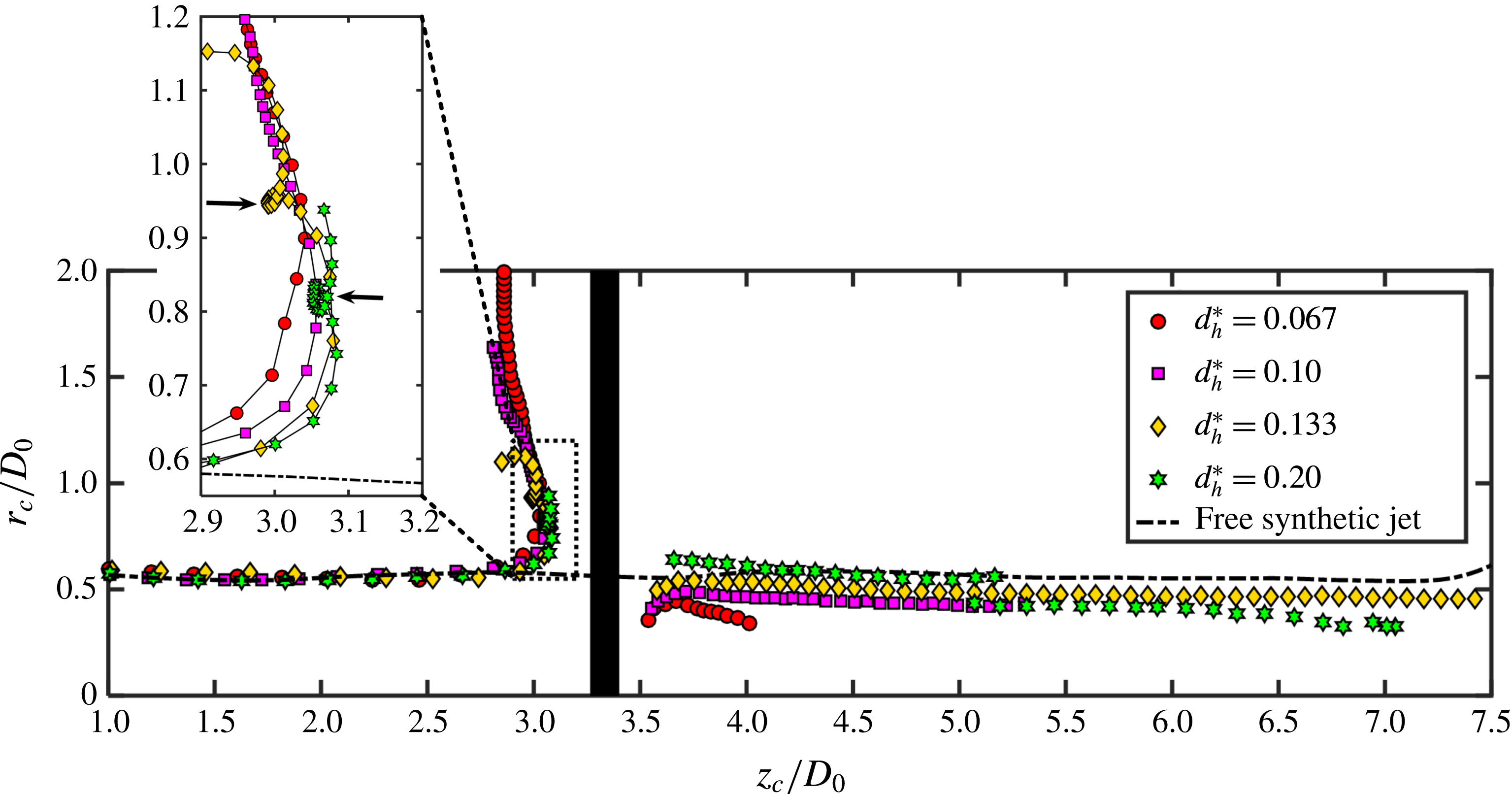
Figure 11. Trajectories of primary (upstream) and transmitted (downstream) vortex rings for all tested cases.

Figure 12. Time evolutions of vortex circulations for all porous wall cases: (a) secondary vortex ring (upstream) and (b) transmitted vortex ring (downstream).

3.4 Vortex ring trajectory and circulation

Although the interaction between the synthetic jet vortex rings and the porous wall shows differences between different jet cycles (figure 10), this study mainly focuses on the process after convergence. Thus, both the vortex ring trajectories and circulations depicted in figures 11 and 12, respectively, are obtained from the phase-averaged vorticity fields. Note that, on the upstream side of the porous wall, the symbols in figure 11 represent the primary vortex ring, while for the downstream side they represent the transmitted vortex ring. Following Feng & Wang (Reference Feng and Wang2010) and Musta & Krueger (Reference Musta and Krueger2014), the vortex centre is defined as the centroid of the vorticity. The location of the vortex centre ( $r_{c},z_{c}$ ) determined for an identified vortical region ( $\unicode[STIX]{x1D6FA}$ ) is expressed as

(3.3a,b ) $$\begin{eqnarray}\displaystyle r_{c}=\frac{\displaystyle \int _{\unicode[STIX]{x1D6FA}}\unicode[STIX]{x1D714}_{\unicode[STIX]{x1D703}}r\,\text{d}\unicode[STIX]{x1D6FA}}{\displaystyle \int _{\unicode[STIX]{x1D6FA}}\unicode[STIX]{x1D714}_{\unicode[STIX]{x1D703}}\,\text{d}\unicode[STIX]{x1D6FA}},\quad z_{c}=\frac{\displaystyle \int _{\unicode[STIX]{x1D6FA}}\unicode[STIX]{x1D714}_{\unicode[STIX]{x1D703}}z\,\text{d}\unicode[STIX]{x1D6FA}}{\displaystyle \int _{\unicode[STIX]{x1D6FA}}\unicode[STIX]{x1D714}_{\unicode[STIX]{x1D703}}\,\text{d}\unicode[STIX]{x1D6FA}}, & & \displaystyle\end{eqnarray}$$

where $\unicode[STIX]{x1D714}_{\unicode[STIX]{x1D703}}$ is the azimuthal vorticity. The vortex circulation $\unicode[STIX]{x1D6E4}$ is calculated as

(3.4) $$\begin{eqnarray}\displaystyle \unicode[STIX]{x1D6E4}=\int _{\unicode[STIX]{x1D6FA}}\unicode[STIX]{x1D714}_{\unicode[STIX]{x1D703}}\,\text{d}\unicode[STIX]{x1D6FA}. & & \displaystyle\end{eqnarray}$$

To determine the vortical region ( $\unicode[STIX]{x1D6FA}$ ), the $\unicode[STIX]{x1D706}_{ci}$ criterion is used to identify vortices in the flow field. In particular, the flow area with a $\unicode[STIX]{x1D706}_{ci}$ value above $0.2~\text{s}^{-1}$ is first recognized as the vortex area. Then, within this vortex area, the region with vorticity magnitude satisfying $\unicode[STIX]{x1D714}_{\unicode[STIX]{x1D703}}/\unicode[STIX]{x1D714}_{\unicode[STIX]{x1D703},p}\geqslant 0.1$ is defined as the final vortical region ( $\unicode[STIX]{x1D6FA}$ ) to eliminate noise from the PIV data (Feng & Wang Reference Feng and Wang2010; Xu et al. Reference Xu, He, Kulkarni and Wang2017), where $\unicode[STIX]{x1D714}_{\unicode[STIX]{x1D703},p}$ represents the local peak vorticity. Both the trajectories and the circulations of the upper and lower halves of the flow domain are averaged to diminish measurement uncertainty. Additionally, the vortex ring trajectory for the free synthetic jet is plotted in figure 11 as a reference.

As shown in figure 11, the vortex ring diameter of the free synthetic jet is equal to approximately $1.1D_{0}$ , slightly larger than the jet nozzle diameter $D_{0}$ , and it is kept nearly constant as it convects downstream (the black dash-dotted line). Moreover, figure 11 depicts that, before the axial location of $z_{c}/D_{0}\approx 2.0$ , the primary vortex ring trajectories for all porous wall cases coincide well with the free jet case, indicating a free development stage. As it approaches the porous wall, the primary vortex ring trajectory begins to spread, leading to an increase in the ring diameter. This phenomenon can be well explained by introducing an image vortex ring with opposite circulation on the other side of the wall, as described by Adhikari & Lim (Reference Adhikari and Lim2009). However, for a porous wall, some fluid passes through the boundary, which weakens the intensity of the image vortex ring. Hence, the primary vortex ring for the case of larger hole diameter stretches across a shorter radial distance (figure 11) because more fluid passes through the porous wall.

A part of the primary vortex ring trajectory (dashed rectangle in figure 11) is enlarged to clearly illustrate the differences between the different cases. It can be observed that for $d_{h}^{\ast }=0.067$ and 0.10, the primary vortex ring continuously spreads radially after rebounding from the wall. This behaviour is similar to that for the synthetic jet vortex rings impacting a solid wall reported by Xu et al. (Reference Xu, Feng and Wang2013, Reference Xu, He, Kulkarni and Wang2017). However, the primary vortex ring experiences a reversal in trajectory at the radial positions of $r_{c}/D_{0}\approx 0.95$ and 0.82 for $d_{h}^{\ast }=0.133$ and 0.20, respectively, as indicated by the black arrows in figure 11. Primary vortex ring reversal has been widely reported in the study of the impingement of a single vortex ring (Walker et al. Reference Walker, Smith, Cerra and Doligalski1987; New, Shi & Zang Reference New, Shi and Zang2016). Walker et al. (Reference Walker, Smith, Cerra and Doligalski1987) attributed this to the intense inviscid interaction between the primary and secondary vortex rings. However, this phenomenon only occurs for porous walls with large hole diameters ( $d_{h}^{\ast }=0.133$ and 0.20).

The discrepancy is attributed first to the vortical structure concentrated near the wall formed by the previously impinged vortex rings. When $d_{h}^{\ast }$ is small, the vortical structure concentrated near the wall upstream suppresses the development of the secondary vortex ring (see figure 6), which weakens the interaction between the primary and secondary vortex rings. However, for large $d_{h}^{\ast }$ , the primary vortex ring swallows the previously impinged vortex ring (see figure 9) and behaves as a single impinging vortex ring after that. Second, for large $d_{h}^{\ast }$ , the bulk of the fluid passes through the porous wall, drawing the primary vortex ring inwards radially. Third, for porous walls with a larger $d_{h}^{\ast }$ , the downstream transmitted vortex ring can induce a stronger velocity on the primary vortex ring pointing to the jet centreline according to the Biot–Savart law. Nonetheless, the primary vortex ring for $d_{h}^{\ast }=0.133$ and 0.20 cannot contract continuously, and it is pushed away after the arrival of the next incident vortex ring, as shown in figure 11. Note that for $d_{h}^{\ast }=0.133$ , the primary vortex ring appears to experience another reversal at $r_{c}/D_{0}>1.05$ . This reversal occurs because the primary vortex ring begins to be swallowed by the next incident vortex ring.

For the downstream flow, figure 11 shows that the transmitted vortex ring diameter increases with the hole diameter ( $d_{h}^{\ast }$ ), and its mean value equals $0.79D_{0}$ , $0.90D_{0}$ , $0.97D_{0}$ and $1.17D_{0}$ for $d_{h}^{\ast }=0.067$ , 0.10, 0.133 and 0.20, respectively. It can be observed that only for $d_{h}^{\ast }=0.20$ is the transmitted vortex ring diameter larger than the vortex ring diameter ( $1.1D_{0}$ ) of the free synthetic jet. Moreover, the transmitted vortex ring for $d_{h}^{\ast }=0.133$ can survive the longest axial distance, as shown in figure 11. It is noticeable that the transmitted vortex ring trajectory for $d_{h}^{\ast }=0.20$ shows a sudden decrease at $r_{c}/D_{0}\approx 5.1$ . This decrease occurs because the transmitted vortex ring is caught up by the discrete jet-like structures (see figure 9 h) formed in the next jet cycle. From figure 11, the convection speed of the vortex ring can be estimated by taking the time derivative of $z_{c}$ . Using the linear fit (correlation coefficient over 0.99), the convection speed of the transmitted vortex ring ( $U_{c}$ ) is calculated to be $3.8~\text{mm}~\text{s}^{-1}$ , $7.4~\text{mm}~\text{s}^{-1}$ , $10.5~\text{mm}~\text{s}^{-1}$ and $8.2~\text{mm}~\text{s}^{-1}$ for $d_{h}^{\ast }=0.067$ , 0.10, 0.133 and 0.20, respectively. For the free synthetic jet, the convection speed of the vortex ring ( $U_{c}$ ) is equal to $19.3~\text{mm}~\text{s}^{-1}$ . Compared with that of the free synthetic jet, the convection speed of the transmitted vortex ring drops by 80 %, 62 %, 46 % and 58 % for $d_{h}^{\ast }=0.067$ , 0.10, 0.133 and 0.20, respectively. Furthermore, the distance between adjacent vortex rings can also be evaluated using $U_{c}\times T_{0}$ , where $T_{0}$ is the synthetic jet excitation period. For the cases of $d_{h}^{\ast }=0.067$ , 0.10, 0.133 and 0.20, the distances between adjacent transmitted vortex rings are equal to 7.6 mm, 14.8 mm, 21 mm and 16.4 mm, respectively, and it is 38.6 mm for the free synthetic jet. As explained by Shuster & Smith (Reference Shuster and Smith2007), the distance between adjacent vortex rings mainly depends on the stroke length of the synthetic jet. Therefore, it can be observed that the modified synthetic jet formed in the porous wall case (explained in figure 4) has a smaller stroke length than that of the incident synthetic jet. It is worth mentioning that, for the free synthetic jet, the distance between adjacent vortex rings (38.6 mm) evaluated based on the convection speed of the vortex ring agrees well with the theoretical value of the stroke length (40.5 mm) presented in table 1.

Figure 12(a,b) presents the evolutions of the circulations for upstream secondary and downstream transmitted vortex rings, respectively. As depicted in figure 12(a), the secondary vortex ring circulation for $d_{h}^{\ast }=0.067$ has two peaks at $t/T_{0}\approx 0.84$ and 1.58, while the single peaks for $d_{h}^{\ast }=0.10$ , 0.133 and 0.20 are located at $t/T_{0}\approx 0.86$ , 0.88 and 0.94, respectively. As explained by Xu et al. (Reference Xu, He, Kulkarni and Wang2017), the rolling up of the secondary vortex ring would produce a peak value in its circulation, while the second peak for $d_{h}^{\ast }=0.067$ might be due to the generation of a tertiary vortex ring. Additionally, figure 12(a) shows that the secondary vortex ring circulation for $d_{h}^{\ast }=0.133$ appears to reach a plateau at $t/T_{0}\approx 1.25$ before the final decay. This plateau should be associated with the pairing between the secondary and primary vortex rings, which drives the vortices to move away from the wall, as illustrated in figure 7. Note that, although vortex pairing also occurs for $d_{h}^{\ast }=0.20$ , the secondary vortex ring is too weak to continuously orbit around the periphery of the primary vortex ring. Thus, no circulation plateau is detected for this case. For the downstream transmitted vortex ring, figure 12(b) shows that all circulations generally first increase then decrease as time evolves. However, for $d_{h}^{\ast }=0.20$ , the transmitted vortex ring circulation experiences a sudden growth at $t/T_{0}\approx 2.14$ , owing to the coalescence with the incoming jet-like structures shown in figure 11. In particular, before the sudden increase in $d_{h}^{\ast }=0.20$ , figure 12(b) shows that the circulation in the case of $d_{h}^{\ast }=0.133$ achieves the maximum among all porous wall cases. For smaller $d_{h}^{\ast }$ (0.067 and 0.10), a weaker transmitted vortex ring occurs because of the passage of less fluid through the porous wall. However, for larger $d_{h}^{\ast }$ (0.20), the reason is that the formation of the discrete jet-like structures weakens the intensity of the downstream transmitted vortex ring.

Figure 13. Dimensionless axial velocity profiles for (a) free synthetic jet, (b) $d_{h}^{\ast }=0.067$ , (c) $d_{h}^{\ast }=0.10$ , (d) $d_{h}^{\ast }=0.133$ and (e) $d_{h}^{\ast }=0.20$ .

Figure 14. Axial evolutions of (a) maximum axial mean velocity $U_{max}$ and (b) jet half-width $r_{1/2}$ for all tested cases.

4.1 Axial jet properties

Figure 13 shows the distributions of the axial mean velocity at different axial locations for all tested cases. The axial mean velocity is normalized by the local maximum velocity ( $U_{max}$ ), and the radial position is scaled by the jet half-width ( $r_{1/2}$ ), which is defined as the location where the velocity decreases to half of $U_{max}$ (Krishnan & Mohseni Reference Krishnan and Mohseni2010; Xu et al. Reference Xu, He, Kulkarni and Wang2017). As depicted in figure 13(a), the velocity profiles for the free synthetic jet collapse reasonably well, particularly at $z/D_{0}\geqslant 6.70$ , indicating self-similar behaviour. This finding is not surprising as James, Jacobs & Glezer (Reference James, Jacobs and Glezer1996), Smith & Glezer (Reference Smith and Glezer1998), Zhang & Wang (Reference Zhang and Wang2007) and Xu et al. (Reference Xu, Feng and Wang2013) demonstrated that the velocity profile for synthetic jets agrees with the hyperbolic cosine function 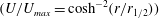$(U/U_{max}=\cosh ^{-2}(r/r_{1/2}))$ , which is denoted by the red dash-dotted line in figure 13. It is noticeable that the velocity profile at $z/D_{0}=0.70$ diverges from the self-similar curve for the free synthetic jet case. This divergence occurs because the flow field close to the jet nozzle is strongly affected by the suction stroke of synthetic jets. Moreover, figure 13(a) shows that, below $U/U_{max}\approx 0.3$ , the velocity profiles in the range $1.70\leqslant z/D_{0}\leqslant 4.70$ appear to be narrower than the fitting curve. This result can be attributed to the passage of the synthetic jet vortex rings, which tends to narrow the jet width, as explained by Shuster & Smith (Reference Shuster and Smith2007).

For the porous wall case, because the mean flow on the upstream side shows features similar to those observed in the free jet case, figure 13(b–e) only presents the velocity profiles in the downstream flow for the sake of brevity. As shown in figure 13(b), for $d_{h}^{\ast }=0.067$ , the velocity profiles of the downstream flow are still generally consistent with the hyperbolic cosine function (red dash-dotted line), except for the region close to the wall ( $z/D_{0}=3.47$ and 3.50). However, for the cases of $d_{h}^{\ast }=0.10$ , 0.133 and 0.20, a finger-type velocity distribution is clearly observed in the region near the wall, and it becomes more wavy as $d_{h}^{\ast }$ increases (figure 13 c–e). Further downstream, this finger-type distribution gradually transitions to a jet-type velocity profile after $z/D_{0}=3.70$ , 4.70 and 4.70 for $d_{h}^{\ast }=0.10$ , 0.133 and 0.20, respectively. This transition should be attributed to vorticity cancellation as well as the formation of transmitted vortex rings. It is important to note that, in the far field of the transmitted jet ( $z/D_{0}\geqslant 6.03$ ), the velocity profiles for all porous wall cases collapse together (see figure 13 b–e) and still coincide with the hyperbolic cosine function (red dash-dotted line). This result indicates that for the current experiment the features of the incident synthetic jet are not fundamentally altered by the porous wall, and the reason should be related to the periodic generation of the transmitted vortex ring downstream.

Figure 14(a,b) shows the axial evolutions of the maximum axial velocity, i.e. jet centreline velocity ( $U_{max}$ ) and jet half-width ( $r_{1/2}$ ), respectively. As depicted in figure 14(a), on the upstream side, the maximum axial velocity ( $U_{max}$ ) for all porous wall cases first increases from the nozzle, reaches a plateau of approximately $1.2U_{0}$ at $z/D_{0}\approx 1.6$ and then decreases rapidly as the jet impacts the wall. For the jet half-width ( $r_{1/2}$ ), figure 14(b) shows that $r_{1/2}$ undergoes a quick growth in the region close to the nozzle, achieves a peak at $z/D_{0}\approx 0.4$ , and then decreases before the second increase caused by impingement. It is observed that, before the axial location of $z/D_{0}\approx 2.0$ , both $U_{max}$ and $r_{1/2}$ for all porous wall cases follow the trend of the free synthetic jet marked by the dash-dotted lines in figure 14. This result indicates that the synthetic jet experiences a free development stage before interacting with the porous wall.

For the transmitted jet downstream, $U_{max}$ first increases and then decreases, while the trend of $r_{1/2}$ is the opposite. The variations of both $U_{max}$ and $r_{1/2}$ are closely associated with the downstream flow structures. Indeed, as explained by Shuster & Smith (Reference Shuster and Smith2007), the discrete vortex rings tend to form a narrow jet, while the vortex rings losing coherence spread the jet width. Accordingly, the formation of the transmitted vortex ring is the reason for the first decrease in $r_{1/2}$ as well as the increase in $U_{max}$ . However, as the transmitted vortex ring convects downstream, it gradually loses coherence (see figures 6 and 7), which results in the following increase in $r_{1/2}$ as well as the decrease in $U_{max}$ . Nonetheless, there are still substantial discrepancies between different porous wall cases. Specifically, for the cases of $d_{h}^{\ast }=0.067$ and 0.10, the axial locations where $r_{1/2}$ begins to increase and where $U_{max}$ starts to decrease are much earlier than that for $d_{h}^{\ast }=0.133$ and 0.20. This result is obtained because, for a small $d_{h}^{\ast }$ , the intensity of the transmitted vortex ring is relatively weak (figure 12 b); hence, it cannot survive a long distance before becoming incoherent (figure 11).

Figure 14(a) shows that $U_{max}$ for $d_{h}^{\ast }=0.20$ appears to undergo the largest decay rate among all porous wall cases in the downstream flow, and after $z/D_{0}\approx 8.5$ its value is even smaller than that for $d_{h}^{\ast }=0.133$ (figure 14 a). This discrepancy can be attributed to the poorly formed transmitted vortex ring in the case of $d_{h}^{\ast }=0.20$ (see figure 9 h), which causes the downstream flow structures to lose coherence more easily. For the free synthetic jet, figure 14 shows that $r_{1/2}$ grows rapidly after $z/D_{0}\approx 6.5$ ; correspondingly, the decay of $U_{max}$ is also accelerated in this region. As a result, after $z/D_{0}\approx 8.0$ , the value of $U_{max}$ for the free synthetic jet case is even lower than that for the porous wall cases of $d_{h}^{\ast }=0.133$ and 0.20. This result is mainly caused by the transition from the periodic vortex rings to a turbulent jet in the free synthetic jet flow. Moreover, as reported by Shuster & Smith (Reference Shuster and Smith2007), the transition of the synthetic jet ended in the axial range between $2.0L_{0}$ and $3.0L_{0}$ ( $L_{0}$ is the stroke length), which contains the location of $6.5D_{0}\approx 2.4L_{0}$ detected in the current experiment. It is worth noting that, because of the formation of the strong finger-type jets, $U_{max}$ for the cases of $d_{h}^{\ast }=0.133$ and 0.20 presents a local peak near the porous wall surface on the downstream side, as shown in figure 14(a).

In summary, for the interaction of the synthetic jet with the porous wall, the fluid passing through the wall would generate a train of transmitted vortex rings (see figure 4), which forms a transmitted jet in the downstream flow field. While the basic features of the synthetic jet are still maintained by the transmitted jet (figure 13), both the intensity (figure 14) and stroke length (figure 11) are reduced compared with those of the incident jet. Nonetheless, because this transmitted jet could be treated as a modified synthetic jet without suction stroke, it would be useful in some applications in which only the vortices are in demand or the suction of synthetic jets has negative effects. On the other hand, under constant surface porosity, the current experiment shows that the synthetic jet vortex rings are heavily disturbed by the porous wall with the largest hole diameter of $d_{h}^{\ast }=0.20$ (see figures 5 and 9). Hence, it can be speculated that the vortex rings would be drastically broken by the porous wall, with no transmitted vortex ring reformed, when the hole diameter grows to a sufficiently large value. This finding certainly provides a strategy for breaking large-scale coherent structures (such as vortex rings) in the flow field for flow control applications.

Figure 15. Axial evolutions of jet (a) flow rate and (b) momentum flux for all tested cases.

4.2 Axial jet entrainment and momentum flux

Flow entrainment and momentum flux are two important parameters for impinging jets as well as their engineering applications. For a synthetic jet impinging onto porous walls, flow entrainment is a key metric for understanding the amount of fresh fluid entrained from the ambient environment and the capacity of mixing in both the upstream and downstream flow fields. Momentum flux provides a useful metric for measuring flow ability in momentum transport as well as revealing the effects of a porous wall on synthetic jets because the drag imposed by the porous wall will remove momentum from the jet flow. Figure 15(a,b) illustrates the variations of the axial flow rate and momentum flux, respectively. Here, the flow rate ( $Q$ ) is calculated by

(4.1) $$\begin{eqnarray}\displaystyle Q=2\unicode[STIX]{x03C0}\int _{0}^{\infty }Ur\,\text{d}r, & & \displaystyle\end{eqnarray}$$

where $U$ is the mean axial velocity and $r$ is the radial location. The flow rate at the jet nozzle ( $Q_{0}$ ) is employed to normalize $Q$ , and $Q_{0}$ is defined as

(4.2) $$\begin{eqnarray}\displaystyle Q_{0}=\frac{\unicode[STIX]{x03C0}D_{0}^{2}}{4}U_{0}. & & \displaystyle\end{eqnarray}$$

The jet momentum flux ( $M$ ) is obtained by the momentum equation for axisymmetric flow provided by Panchapakesan & Lumley (Reference Panchapakesan and Lumley1993):

(4.3) $$\begin{eqnarray}\displaystyle M=2\unicode[STIX]{x03C0}\unicode[STIX]{x1D70C}\int _{0}^{\infty }\left(U^{2}+u_{rms}^{2}-\frac{1}{2}v_{rms}^{2}\right)r\,\text{d}r, & & \displaystyle\end{eqnarray}$$

where $u_{rms}$ and $v_{rms}$ are the axial and radial root-mean-square velocities, respectively. Similarly, $M$ is scaled by the jet nozzle momentum flux ( $M_{0}$ ), which is expressed as

(4.4) $$\begin{eqnarray}\displaystyle M_{0} & = & \displaystyle \frac{1}{T_{0}}\int _{0}^{T_{0}/2}\unicode[STIX]{x1D70C}\int _{0}^{D_{0}/2}u_{0}^{2}(t)\,2\unicode[STIX]{x03C0}r\,\text{d}r\,\text{d}t\approx \frac{1}{T_{0}}\int _{0}^{T_{0}/2}\unicode[STIX]{x1D70C}u_{0}^{2}(t)\,\frac{1}{4}\unicode[STIX]{x03C0}D_{0}^{2}\,\text{d}t\nonumber\\ \displaystyle & = & \displaystyle \frac{\unicode[STIX]{x03C0}^{3}\unicode[STIX]{x1D70C}U_{0}^{2}D_{0}^{2}}{16}.\end{eqnarray}$$

Both the flow rates and momentum fluxes above and below the jet centreline are averaged together to help to diminish the measurement uncertainty.

As shown in figure 15(a), the flow rate $Q$ for all porous wall cases increases quickly (approximately linear) from the nozzle, achieves a peak at $z/D_{0}\approx 2.0$ and then decreases on approaching the porous wall. Beyond $z/D_{0}\approx 4.0$ downstream, an approximately linear growth of $Q$ is observed for the transmitted jets for all porous wall cases. Additionally, in the downstream flow, figure 15(a) shows that a larger hole diameter ( $d_{h}^{\ast }$ ) produces a higher value of $Q$ at the same axial location. As suggested by Greco et al. (Reference Greco, Cardone and Soria2017), the axial derivative of $Q$ can be defined as entrainment ( $\unicode[STIX]{x1D700}$ ), which reflects the ability of a jet to entrain the surrounding fluid:

(4.5) $$\begin{eqnarray}\displaystyle \unicode[STIX]{x1D700}=\frac{\text{d}Q}{\text{d}z}=\frac{\text{d}}{\text{d}z}\left[2\unicode[STIX]{x03C0}\int _{0}^{\infty }Ur\,\text{d}r\right]. & & \displaystyle\end{eqnarray}$$

Using the linear fit (correlation coefficient over 0.99), the dimensionless entrainment ( $\unicode[STIX]{x1D700}/U_{0}D_{0}$ ) of the transmitted jet ( $z/D_{0}\geqslant 4.0$ ) is calculated to be 0.036, 0.046, 0.072 and 0.11 for $d_{h}^{\ast }=0.067$ , 0.10, 0.133 and 0.20, respectively. For $d_{h}^{\ast }=0.067$ , 0.10 and 0.133, the increase in the entrainment with $d_{h}^{\ast }$ is due to the strengthened transmitted vortex ring in the downstream flow (see figure 12 b), which helps engulf more fluid from the surrounding environment. For $d_{h}^{\ast }=0.20$ , although figure 12(b) shows that its transmitted vortex ring has a lower intensity than that for $d_{h}^{\ast }=0.133$ , the ring is more disturbed because of the formation of discrete jet-like structures (figure 9 h). Thus, the downstream vortical structures for this case would lose coherence easily or even probably transition to turbulence. This effect is helpful for promoting the entrainment ability of the downstream transmitted jet. For the free synthetic jet, figure 15(a) shows that $Q$ undergoes two linear growth stages at $0.2<z/D_{0}<2.0$ and at $z/D_{0}>6.5$ , which correspond to the generation of the vortex rings and the transition to turbulent flow, respectively. Using the above-mentioned linear fit, $\unicode[STIX]{x1D700}/U_{0}D_{0}$ for $0.2<z/D_{0}<2.0$ and $z/D_{0}>6.5$ are calculated to be 0.33 and 0.54, respectively, both of which are much larger than that for the transmitted jet. It can be observed that the capacity for entrainment could be greatly improved after the flow transitions to turbulence.

For the momentum flux ( $M$ ) upstream, figure 15(b) shows that $M$ for all porous wall cases grows rapidly near the nozzle, reaches a local peak at $z/D_{0}\approx 0.2$ and then falls to a nearly constant value. As the jet approaches the porous wall, $M$ undergoes another increase for all porous wall cases and achieves a second peak at $z/D_{0}\approx 3.0$ before the final reduction. Additionally, the smaller the hole diameter ( $d_{h}^{\ast }$ ) is, the higher will be the second peak of $M$ . This second growth of $M$ might be related to the accumulation of the jet momentum as the vortex rings continuously impact the wall, as well as the fact that the stretching of the vortex ring would widen the jet width and enhance the magnitude of the axial velocity fluctuations.

For the transmitted jet downstream, $M$ for all porous wall cases appears to achieve an approximately constant value at $M/M_{0}=0.024$ , 0.085, 0.16 and 0.21 for $d_{h}^{\ast }=0.067$ , 0.10, 0.133 and 0.20, respectively. As expected, the removal of $M$ by the porous wall decreases with the increase in $d_{h}^{\ast }$ . For the free synthetic jet, after the rapid growth near the nozzle, $M$ undergoes a slow decrease until $z/D_{0}\approx 6.5$ , where the jet flow transitions to turbulence as previously explained. The momentum loss for the free synthetic jet might be attributed to ‘back-flow’ in the ambient fluid caused by the ease with which the jet is confined here (?Musta & Krueger Reference Musta and Krueger2015). Beyond $z/D_{0}\approx 6.5$ , $M$ for the free synthetic jet could be roughly regarded as constant; so the fractional decrease in $M$ caused by the presence of the porous wall is estimated to be 95 %, 81 %, 64 % and 53 % for $d_{h}^{\ast }=0.067$ , 0.10, 0.133 and 0.20, respectively. Again, in the free development stage at $z/D_{0}<2.0$ , the evolutions of both $Q$ and $M$ for all porous wall cases agree well with that for the free synthetic jet, as shown in figure 15.

Figure 16. Basic diagram of the control-volume approach for determining the force of a porous wall.

4.3 Estimation of the porous wall drag based on PIV measurements

For practical applications of porous media, drag is an important aspect that must be considered. For instance, in designing wind/water tunnel settling chambers, lower drag along the flow straightener with no effects on flow quality is always expected in order to save more power consumption. Another example is heat exchangers; the porous medium applied in this case usually features a large surface area to increase the heat transfer coefficient, which comes at the expense of increased flow resistance decreasing convection. Therefore, for the current study, the drag force of the porous wall is evaluated from the PIV-measured velocity fields using the control-volume approach. Considering a control volume ( $V$ ) across the porous wall shown in figure 16, the integral momentum equation for the incompressible flow can be written as (Kurtulus, Scarano & David Reference Kurtulus, Scarano and David2007)

(4.6) $$\begin{eqnarray}\displaystyle \boldsymbol{F}(t)=-\unicode[STIX]{x1D70C}\iiint _{V}\frac{\unicode[STIX]{x2202}\boldsymbol{u}}{\unicode[STIX]{x2202}t}\cdot \text{d}V-\unicode[STIX]{x1D70C}\iint _{S}(\boldsymbol{u}\boldsymbol{\cdot }\boldsymbol{n})\boldsymbol{u}\boldsymbol{\cdot }\text{d}s-\iint _{S}p\boldsymbol{n}\boldsymbol{\cdot }\text{d}s+\iint _{S}\bar{\bar{\unicode[STIX]{x1D70F}}}\boldsymbol{u}\boldsymbol{\cdot }\text{d}s,\quad & & \displaystyle\end{eqnarray}$$

where $\boldsymbol{F}$ is the force vector, $S$ is the outer surface of the control volume $V$ , $\boldsymbol{n}$ represents the normal direction of $S$ , $\boldsymbol{u}$ is the velocity vector, $p$ is pressure and $\bar{\bar{\unicode[STIX]{x1D749}}}$ is the viscous stress tensor.

From (4.6), it can be observed that, if one tries to obtain the force $\boldsymbol{F}$ , the instantaneous fluid velocity within $V$ and the pressure distribution on $S$ should be known because the viscous stress tensor can be calculated from the velocity information. Fortunately, for experimentalists, the instantaneous velocity information can be obtained via the PIV technique, while the corresponding pressure can be resolved through a velocity-gradient-integration scheme (Liu & Katz Reference Liu and Katz2013; Dabiri et al. Reference Dabiri, Bose, Gemmell, Colin and Costello2014; Wang et al. Reference Wang, Gao, Wang, Wei and Wang2016) or by solving the Poisson equation (Gresho & Sani Reference Gresho and Sani1987; Gurka et al. Reference Gurka, Liberzon, Hefetz, Rubinstein and Shavit1999; Vanierschot & van den Bulck Reference Vanierschot and van den Bulck2008). Theoretically, the instantaneous pressure could be obtained from the instantaneous PIV velocity by using the above-mentioned principles; however, it is not easy to guarantee a sufficient level of accuracy for each instantaneous pressure field. Moreover, in most application scenarios, the technical concern mainly focuses on the mean characteristics required of the mean pressure field and force. In this context, the time-mean force can be calculated by averaging (4.6) over time and is expressed as

(4.7) $$\begin{eqnarray}\displaystyle \bar{F}_{i} & = & \displaystyle -\unicode[STIX]{x1D70C}\iint _{S}\bar{u}_{i}\bar{u}_{j}\cdot n_{j}\,\text{d}s-\unicode[STIX]{x1D70C}\iint _{S}\overline{u_{i}^{\prime }u_{j}^{\prime }}\cdot n_{j}\,\text{d}s\nonumber\\ \displaystyle & & \displaystyle -\,\iint _{S}\bar{p}\cdot n_{i}\,\text{d}s+\unicode[STIX]{x1D707}\iint _{S}\left(\frac{\unicode[STIX]{x2202}\bar{u}_{i}}{\unicode[STIX]{x2202}x_{j}}+\frac{\unicode[STIX]{x2202}\bar{u}_{j}}{\unicode[STIX]{x2202}x_{i}}\right)\cdot n_{j}\,\text{d}s,\end{eqnarray}$$

where $\bar{F}_{i}$ and $\bar{u}_{i}$ are the time-mean force and velocity components and $x_{i}$ , $\bar{p}$ and $\unicode[STIX]{x1D707}$ denote the coordinate location, the mean pressure and the dynamic viscosity of the fluid, respectively. The terms on the right-hand side of (4.7) represent the contributions to the total force from the mean and turbulent momentum transfers, the pressure distribution and the viscous stress, respectively (Kurtulus et al. Reference Kurtulus, Scarano and David2007). For the axisymmetric flow here, all terms on the right-hand side of (4.7) except the mean pressure ( $\bar{p}$ ) could be obtained from the mean and statistical velocities and their gradients delivered by planar PIV measurements across the axisymmetric plane.

It is well known that, for incompressible flow, the time-mean pressure $\bar{p}$ is determined by the time-mean Poisson equation (van Oudheusden Reference van Oudheusden2013):

(4.8) $$\begin{eqnarray}\displaystyle \unicode[STIX]{x1D6FB}^{2}\bar{p}=-\unicode[STIX]{x1D70C}\unicode[STIX]{x1D735}\boldsymbol{\cdot }(\bar{\boldsymbol{u}}\boldsymbol{\cdot }\unicode[STIX]{x1D735})\bar{\boldsymbol{u}}-\unicode[STIX]{x1D70C}\unicode[STIX]{x1D735}\boldsymbol{\cdot }\unicode[STIX]{x1D735}\boldsymbol{\cdot }(\overline{\boldsymbol{u}^{\prime }\boldsymbol{u}^{\prime }}), & & \displaystyle\end{eqnarray}$$

where $\unicode[STIX]{x1D735}$ is the gradient operator, $\bar{\boldsymbol{u}}$ is the mean velocity and $\overline{\boldsymbol{u}^{\prime }\boldsymbol{u}^{\prime }}$ denotes the Reynolds stress term. As suggested by Gresho & Sani (Reference Gresho and Sani1987), the boundary condition for (4.8) can be derived by applying the time-mean Navier–Stokes equation to the boundary of the solution domain (Neumann condition):

(4.9) $$\begin{eqnarray}\displaystyle \left(\unicode[STIX]{x1D735}\bar{p}=-\unicode[STIX]{x1D70C}(\bar{\boldsymbol{u}}\boldsymbol{\cdot }\unicode[STIX]{x1D735})\bar{\boldsymbol{u}}-\unicode[STIX]{x1D70C}\unicode[STIX]{x1D735}\boldsymbol{\cdot }(\overline{\boldsymbol{u}^{\prime }\boldsymbol{u}^{\prime }})+\unicode[STIX]{x1D707}\unicode[STIX]{x1D6FB}^{2}\bar{\boldsymbol{u}}\right)_{on\;boundary}. & & \displaystyle\end{eqnarray}$$

Therefore, by virtue of the PIV measured velocity, the time-mean pressure field could be attained by numerically solving (4.8) and (4.9). For this study, the flow is regarded as axisymmetric; therefore, the equations used in the pressure evaluation are expressed in cylindrical coordinates (Vanierschot & van den Bulck Reference Vanierschot and van den Bulck2008). Additionally, both Maxworthy (Reference Maxworthy1977) and Gan, Dawson & Nickels (Reference Gan, Dawson and Nickels2012) indicate that vortex rings possess a weak azimuthal velocity; thus, it is reasonable to treat the azimuthal velocity of the laminar vortex ring as zero for the current experiment. The basic procedure for solving the time-mean Poisson equation is similar to that described by Wang et al. (Reference Wang, Gao, Wang, Wei and Wang2016). A second-order central difference scheme is applied to calculate the Laplacian operator as well as the spatial gradients.

In the current study, the porous wall completely divides the PIV measurement domain into upstream and downstream parts; thus, the pressure must be evaluated on these two parts separately. As explained by Dabiri et al. (Reference Dabiri, Bose, Gemmell, Colin and Costello2014), evaluating the pressure by solving the Poisson equation is sensitive to the boundary condition, whose error could be accumulated to affect the entire pressure field. Therefore, the domains over which the pressure is solved for both the upstream and downstream fields are located 3.0 mm (1.4 times the axial scale of the interrogation window) from the porous wall surface, as indicated by the blue rectangles in figure 17(a). This value is established to avoid large uncertainty in the PIV measurements in the near-wall region. After the time-mean pressure fields are resolved separately, it is necessary to unify them through pressure calibration. Considering the low Reynolds number ( $Re_{sj}=308$ ) and the relatively large radial range of the PIV measurement domain ( $4.2D_{0}$ shown in figure 17(a), $D_{0}$ is the nozzle diameter), the fluid motion at the top and bottom edges of the FOV should be weak. On the upstream side, the suction stroke of the synthetic jet would affect the flow area near the jet nozzle (Shuster & Smith Reference Shuster and Smith2007); additionally, a wall jet might appear in the region close to the porous wall (Webb & Castro Reference Webb and Castro2006). Hence, the upstream pressures at the top and bottom edges of $1.5<z/D_{0}<2.0$ are averaged to be equal to the ambient pressure $p_{\infty }$ . For the downstream flow, this average is calculated over the axial range of $4.0<z/D_{0}<4.5$ to avoid significant jet spreading. Indeed, both the velocity and velocity fluctuations at the edges of the chosen ranges (i.e. $1.5<z/D_{0}<2.0$ upstream, $4.0<z/D_{0}<4.5$ downstream) are quite small; thus, the flow could be approximately treated as ‘quiet’.

Figure 17. (a) Schematic of time-mean pressure-solving domain. (b) Calibrated time-mean pressure field for $d_{h}^{\ast }=0.133$ . Positive and negative pressures are represented by solid and dashed lines, respectively. The contour intervals for the upstream and downstream sides are 0.03 and 0.015, respectively.

Figure 17(b) depicts the calibrated time-mean pressure field for the case of $d_{h}^{\ast }=0.133$ , where the pressure is normalized as $(\,\bar{p}-p_{\infty })/(\unicode[STIX]{x1D70C}U_{0}^{2}/2)$ . Because the other porous wall cases present a similar distribution of the time-mean pressure, they are not presented, for the sake of brevity. It can be observed that, on the upstream side, the mean pressure has two negative concentration regions before $z/D_{0}=2.0$ , which correspond to the passage of the synthetic jet vortex rings. Beyond $z/D_{0}=2.5$ , figure 17(b) shows that a positive concentration region appears and the negative pressure spreads radially. These phenomena are due to the deceleration and the stretching of the primary vortex ring caused by the interaction with the porous wall. In the region near the porous wall (such as $z/D_{0}=3.0$ ), one can observe that the fluid would first experience a favourable pressure gradient followed by an adverse one as it spreads radially from the centreline ( $r/D_{0}=0$ ). Under the effect of this adverse pressure gradient, the fluid separates from the wall to form a secondary vortex ring, as illustrated in figures 6 and 7. On the downstream side, figure 17(b) shows that before $z/D_{0}\approx 4.7$ the mean pressure also has two negative concentration regions. These regions are associated with the formation of the transmitted vortex ring. Beyond $r/D_{0}\approx 5.0$ , the pressure gradually recovers to be equal to the ambient pressure. Further downstream, it can be observed that the time-mean pressure increases slightly, as depicted in figure 17(b). This effect might be attributed to the jet spreading in the far field and the ease with which the jet is confined (Musta & Krueger Reference Musta and Krueger2015).

Figure 18. Variation of time-mean drag of porous wall with the control-volume size $H$ . The black dashed line represents the mean drag averaged over different control-volume sizes.

After the time-mean pressure field is acquired, the time-mean drag of the porous wall can be calculated by applying the control-volume approach expressed in (4.7). To validate the reliability of the method, figure 18 presents the variation of the time-mean drag (normalized as $F_{D}/\unicode[STIX]{x1D70C}(U_{0}D_{0})^{2}$ ) with the control-volume size ( $H$ in figure 16). It is well known that there is no object inside a free jet flow; therefore, the drag force for the free jet should theoretically be zero. As shown in figure 18, the calculated drag of the free synthetic jet (brown dashed line) is very small, with the mean value equalling 0.023, which is one order of magnitude lower than the porous wall cases. Moreover, figure 18 shows that all calculated time-mean drags remain nearly constant with the increase in the control-volume size ( $H$ ). Therefore, it can be concluded that both the data and the method employed in this study are reasonably accurate and reliable, at least for the time-mean flow. Note that the lack of true flow axisymmetry would introduce bias errors in the pressure evaluation as well as in determining the time-mean drag. Nevertheless, the results evaluated herein can still be expected to reliably reflect the trend of the drag force for comparison between porous walls with different hole diameters ( $d_{h}^{\ast }$ ). The black dashed lines in figure 18 denote the mean drag ( $\bar{F}_{D}/\unicode[STIX]{x1D70C}(U_{0}D_{0})^{2}$ ) averaged over different control-volume sizes. For the cases of $d_{h}^{\ast }=0.067$ , 0.10, 0.133 and 0.20, the mean drag is equal to approximately 0.80, 0.74, 0.54 and 0.43, respectively. As expected, the time-mean drag decreases with the increase in $d_{h}^{\ast }$ . For $d_{h}^{\ast }=0.067$ and 0.10, the deviation of $F_{D}$ from its mean value appears to be more significant than that for $d_{h}^{\ast }=0.133$ and 0.20. This result should be associated with the formation of a stronger wall jet in the upstream flow, which would introduce greater uncertainty into the pressure calibration for the smaller $d_{h}^{\ast }$ .

4.4 Further analysis on the porous wall drag

According to Darcy’s law refined by Muskat & Botset (Reference Muskat and Botset1931), the pressure drop ( $\unicode[STIX]{x0394}p$ ) imposed by a porous medium is proportional to the product of the flow rate through the porous medium ( $Q$ ) and the dynamic fluid viscosity ( $\unicode[STIX]{x1D707}$ ), and inversely proportional to the product of the permeability ( $K$ ) and the cross-sectional flow area ( $A$ ):

(4.10) $$\begin{eqnarray}\displaystyle \frac{\unicode[STIX]{x0394}p}{L_{h}}=\frac{\unicode[STIX]{x1D707}Q}{KA}, & & \displaystyle\end{eqnarray}$$

where $L_{h}$ is the length of the porous medium. When considering a uniform incoming flow, (4.10) can be rewritten as

(4.11) $$\begin{eqnarray}\displaystyle \frac{\unicode[STIX]{x0394}p}{L_{h}}=\frac{\unicode[STIX]{x1D707}}{K}u, & & \displaystyle\end{eqnarray}$$

where $u=Q/A$ is the flow velocity. In fact, (4.11) is the original form of Darcy’s law; Muskat & Botset (Reference Muskat and Botset1931) first refined it as (4.10) to satisfy the demands of engineering applications. Note that, although the permeability $K$ is defined based on Darcy’s equation, it is a characteristic parameter of porous media. In fact, $K$ is only determined by the internal structure of a porous medium and has no relationship with the incident flow condition or the porous medium length (Lage, Krueger & Narasimhan Reference Lage, Krueger and Narasimhan2005). It is worth mentioning that Darcy’s law is a first-order model and is only applicable when the flow velocity is low (i.e. viscous effects are dominated). As the velocity becomes high, a quadratic term associated with form drag must be taken into account to provide a better description of the pressure drop, which is known as the Hazen–Dupuit–Darcy (HDD) equation (Wilson, Narasimhan & Venkateshan Reference Wilson, Narasimhan and Venkateshan2006; Naaktgeboren, Krueger & Lage Reference Naaktgeboren, Krueger and Lage2012b ). Considering the low Reynolds number as well as the limited data in the current experiment, Darcy’s law is employed merely to evaluate the magnitude of the permeability of the porous wall.

Both the left- and right-hand sides of (4.10) are multiplied by the cross-sectional area $A$ (here is the radial range of FOV), and the equation is rewritten as

(4.12) $$\begin{eqnarray}\displaystyle K=\frac{\unicode[STIX]{x1D707}QL_{h}}{F_{D}}, & & \displaystyle\end{eqnarray}$$

where $F_{D}=\unicode[STIX]{x0394}p\,A$ is the drag of the porous wall and $L_{h}=2.0~\text{mm}$ is the thickness of the porous wall. All calculations are based on the time-mean flow field; thus, the parameters on the right-hand side of (4.12) should be the time-mean values. The grid of the PIV velocity field closest to the porous wall surface is used to estimate the flow rate ( $Q$ ) passing through the porous wall. Additionally, the flow rates calculated on both the upstream and downstream sides are averaged together to improve the accuracy of  $Q$ .

Figure 19. Variation of permeability with the square of the hole diameter for the current experiment.

Figure 19 shows the evaluated permeability $K$ for all experimental porous walls. It can be observed that $K$ generally increases with the growth of the hole diameter ( $d_{h}^{\ast }$ ) and equals $1.89\times 10^{-8}~\text{m}^{2}$ , $4.43\times 10^{-8}~\text{m}^{2}$ , $8.24\times 10^{-8}~\text{m}^{2}$ and $11.9\times 10^{-8}~\text{m}^{2}$ for $d_{h}^{\ast }=0.067$ , 0.10, 0.133 and 0.20, respectively. Note that the value of $K$ calculated here is of the same order of magnitude as that measured by Wilson et al. (Reference Wilson, Narasimhan and Venkateshan2006), whose porous media featured a geometry similar to ours. This result verifies the accuracy of the data used in this study and further implies that Darcy’s law appears to be reasonably applicable to the current porous wall. On the other hand, before $(d_{h}^{\ast })^{2}=0.018$ , the permeability $K$ appears to grow linearly with $(d_{h}^{\ast })^{2}$ , while as $(d_{h}^{\ast })^{2}$ increases to 0.04 the value of $K$ becomes much smaller relative to the linear trend, as indicated by the red dashed line in figure 19. The first linear dependence might be explained by the Hagen–Poiseuille equation, which describes the pressure drop caused by viscous effects for laminar flow through a long pipe (Sutera & Skalak Reference Sutera and Skalak1993):

(4.13) $$\begin{eqnarray}\displaystyle \unicode[STIX]{x0394}p=\frac{128\unicode[STIX]{x1D707}L_{cp}Q}{\unicode[STIX]{x03C0}d_{cp}^{4}}, & & \displaystyle\end{eqnarray}$$

where $L_{cp}$ is the pipe length, $Q$ is the flow rate and $d_{cp}$ is the pipe diameter. For the current experiment, the jet width is much larger than the hole diameter (figure 14 b); thus, each hole on the porous wall could be approximately treated as a small pipe. Applying the Hagen–Poiseuille equation to the hole leads to

(4.14) $$\begin{eqnarray}\displaystyle \unicode[STIX]{x0394}p_{h}\sim \frac{\unicode[STIX]{x1D707}L_{h}Q_{h}}{d_{h}^{4}}, & & \displaystyle\end{eqnarray}$$

where $Q_{h}$ is the flow rate through the hole. It should be noted that although the Hagen–Poiseuille equation is applicable to a long pipe or fully developed flow, which is not the case in this study, it can still be used to estimate the magnitude of the pressure drop imposed by a hole. Thus, (4.14) is written in a correlative form and not as an equality. The drag force ( $F_{D_{h}}$ ) caused by a hole can therefore be evaluated as

(4.15) $$\begin{eqnarray}\displaystyle F_{D_{h}}\sim \frac{\unicode[STIX]{x1D707}L_{h}Q_{h}}{d_{h}^{2}}. & & \displaystyle\end{eqnarray}$$

Because $F_{D}$ should be proportional to the sum of $F_{D_{h}}$ , a comparison of (4.12) with (4.15) indicates that the permeability $K$ is linearly dependent on $(d_{h}^{\ast })^{2}$ . This finding exactly matches the experimental behaviour of $K$ before $(d_{h}^{\ast })^{2}=0.018$ presented in figure 19. Therefore, it could be concluded that, for the current experiment, the drag of porous walls with a small hole diameter ( $d_{h}^{\ast }=0.067$ , 0.10 and 0.133) appears to derive mainly from the viscous effect. The deviation of $(d_{h}^{\ast })^{2}=0.04$ from the linear trend should be associated with the increased form drag. Both Boomsma & Poulikakos (Reference Boomsma and Poulikakos2002) and Lage et al. (Reference Lage, Krueger and Narasimhan2005) found that the form drag of porous media is comparable to the viscous drag when the $d_{h}$ -based Reynolds number $Re_{h}$ is greater than $O(1)$ ( $Re_{h}=\unicode[STIX]{x1D70C}u_{h}d_{h}/\unicode[STIX]{x1D707}$ , $u_{h}$ is the fluid velocity through the hole). Although the simulation results of Naaktgeboren et al. (Reference Naaktgeboren, Krueger and Lage2012b ) argue that this criterion is too conservative, here the maximum $Re_{h}$ (based on the mean flow) for $(d_{h}^{\ast })^{2}=0.04$ is greater than 60, largely exceeding the above-mentioned criterion. Additionally, as $d_{h}^{\ast }$ becomes large, the relative length of the hole ( $L_{h}/d_{h}$ ) is further shortened, causing the Hagen–Poiseuille equation to be less applicable. As a result, the enhanced form drag is incorporated into the permeability, leading to a relatively smaller $K$ for $(d_{h}^{\ast })^{2}=0.04$ compared with the linear trend (figure 19).

In summary, when the hole diameter is small (such as $d_{h}^{\ast }=0.067$ , 0.10 and 0.133), the viscous effect appears to be the main source of the total drag of the porous wall. However, for the large hole diameter case ( $d_{h}^{\ast }=0.20$ ), the form drag associated with the geometry of the porous wall becomes significant. Thus, the HDD equation and further experiments are needed to model the hydraulic properties of this type of porous wall.