2.1. Basic idea

In recent research on automatic route generation, the algorithm of the route binary tree based on a single chart is one of the most common approaches and its basic idea is as follows: First, a representation of the obstacles that threaten the safety of ship navigation is constructed by analysing and modelling chart data. Then, the mechanism of automatically keeping away from the obstacles is designed and thus, a feasible route is generated.

2.2. Obstacle representation based on a single chart

To automatically generate safe and reliable routes, the concept of obstacles is proposed and used to describe the sea area where the ship cannot navigate (Zhang, Reference Zhang2011; Chang et al., Reference Chang, Jan and Parberry2004; Szlapczynski, Reference Szlapczynski2006). Based on the existing studies, the obstacles mainly include shallow depth obstacles (for example, land area, island area, rocks) and man-made obstacles (for example, prohibited area, shipwreck area) (Zhang et al., Reference Zhang, Zhang, Peng, Li and Zou2011). These obstacles can be extracted from the chart. The specific method is as follows.

First, the shallow areas are extracted. Based on the sounding points from the chart, a depth model can be constructed with a Triangulated Irregular Network (TIN) (Zhang et al., Reference Zhang, Zhu, Zhang, Liu and Han2008). Considering the ship's draft, the safe depth contours are traced from the depth model, and thus the shallow depth areas are acquired (Zhang, Reference Zhang2011; Zhang et al., Reference Zhang, Zhu, Zhang, Liu and Han2008; Peters et al., Reference Peters, Ledoux and Meijers2014; Guilbert, Reference Guilbert2016).

Second, the man-made areas are extracted. According to the chart area data attributes, man-made obstacles can be easily extracted from the chart.

The ocean environment is complex and changeable, and some factors (for example, the ship's circumflex radius and positioning accuracy) must be considered when designing routes (Pietrzykowski and Uriasz, Reference Pietrzykowski and Uriasz2009; Jones and Rowe, Reference Jones and Rowe2016). Therefore, obstacle areas should be extended with a certain buffer. As some obstacle areas may intersect after the buffer is added, the obstacle areas need to be assessed and simplified to ensure the validity of the topological relationships of the obstacle areas. As shown in Figure 1, the obstacle areas are represented in one chart area.

Figure 1. Representation of obstacles in the chart area.

2.3. Automatic route generation based on the route binary tree

After extracting obstacle areas, the next step is to generate a route. The automatic generation of the shortest distance route means finding the shortest path from the starting point to the destination, for which the classic method is the route binary tree algorithm (Wang et al., Reference Wang, Chen and Zhang2005; Cao et al., Reference Cao, Zhang, Jia and Zhang2011; Wang et al., Reference Wang, Zhang, Peng, Cao and Jiang2016a; Reference Wang, Zhang, Peng, Cao and Jiang2016b).

As shown in Figure 2(a), the starting point is S, the destination point is T, and the obstacle areas are O ₁ and O ₂. The basic principle of the route binary tree algorithm is as follows:

1. (1) Take the starting point S as the current test point and find the nearest obstacle area O ₁ from which the vessel at the current test point needs to keep away.

2. (2) Determine the left child node P ₁ and the right child node P ₃ and establish the route binary tree.

3. (3) Regard the child nodes P ₁ and P ₃ as the current test points, and repeat steps (1) and (2) until there are no obstacle areas from the test points to the terminal point T.

4. (4) Build a route binary tree as shown in Figure 2(b), and then calculate the distance between the nodes and store it in the data structure of the route binary tree.

5. (5) Search the data structure of the route binary tree from top to bottom and sum up the distance of all optional routes and select the shortest one. For this example, the shortest route is SP ₃P ₄P ₅P ₆T.

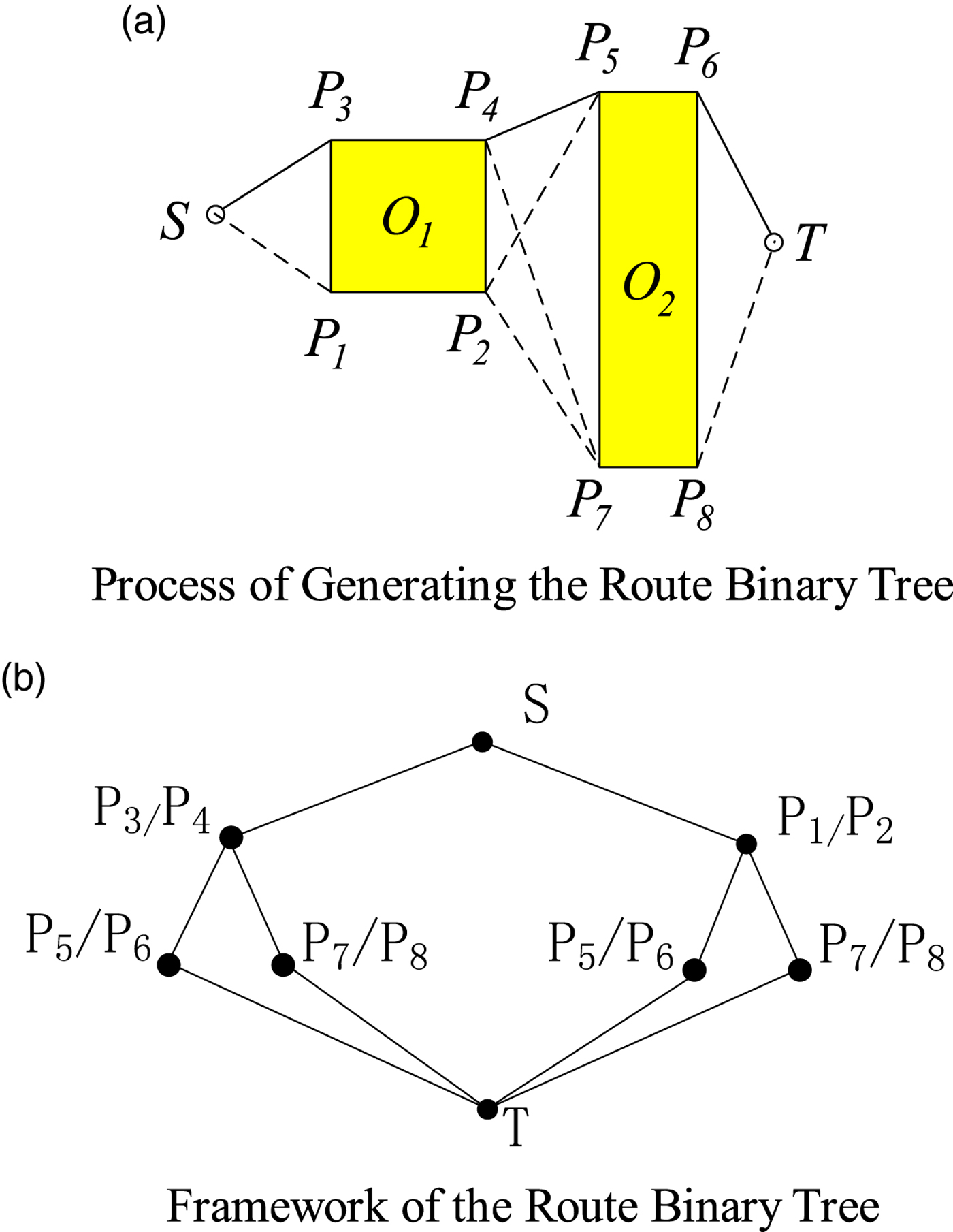
Figure 2. Route Generation Based on the Route Binary Tree.

3.1. Basic idea

The existing binary tree algorithm can generate the shortest route between any two points on a single chart. However, one chart alone is generally not enough for a ship's navigation. While two (or more) charts are utilised, the existing algorithms cannot be adopted to generate routes. Therefore, a new method is proposed in this paper, and its basic idea is as follows:

1. (1) Fuse the obstacle data extracted from different charts. Obstacle data extracted from different charts are compared and analysed quantitatively, and the model fusing all the obstacle data is constructed. Thus, the obstacles from different charts can be represented together with a high accuracy.

2. (2) Building and updating the obstacle spatial database. A spatial database is built for storing obstacle data fused from the different charts. In addition, considering the influence of chart correction and reproduction, a mechanism is designed for sorting and updating the obstacle data.

3. (3) Optimising the efficiency of the algorithm. With the obstacle data fused from multiple charts, the amount of data may become increasingly large. Considering the influence of the amount of data on the algorithm, a route window and an improved R-tree index are proposed for quickly searching and extracting the obstacles.

3.2. Fusing the obstacle data extracted from the different charts

A small-scale chart cannot accurately preserve all the data from a large-scale chart (Yan et al., Reference Yan, Guilbert and Saux2016). Therefore, a cartographic generalisation should be performed to simplify the data from the large-scale chart to be compatible with that from a small-scale chart, and hence the accuracy is decreased.

As shown in Figure 3, the obstacles extracted from two charts with different scales represent the same sea area. The obstacles extracted from the chart with a small scale are shown in Figure 3(a), and the obstacles from the chart with a large scale are shown in Figure 3(b). It can be concluded that, the larger the chart scale, the higher the chart accuracy, but the smaller the sea area covered; on the other hand, the smaller the chart scale, the larger the sea area covered, but the lower the chart accuracy. In Figure 3, it is shown that some navigable areas such as the narrow channel and waterway shown in Figure 3(b) are represented as non-navigable areas in Figure 3(a), and even some non-navigable areas in Figure 3(b) are represented as navigable areas in Figure 3(a), so that the navigational safety of a ship might be threatened. If the distance between the start point and the end point is so far that the chart with the large scale cannot overlay both points, the existing method for generating a ship route only utilises the chart with the small scale, which can overlay both the start point and the end point, thereby decreasing the reliability of the generated route.

Figure 3. Representation of obstacles extracted from different charts.

For generating a route with high reliability, a model for fusing the obstacle data extracted from different charts is constructed in this paper. The specific method is as follows:

1. (1) For quantitatively comparing the accuracy of two (or more) charts, an index of accuracy is defined. Usually, the chart accuracy is positively related to the chart scale. In other words, the larger the chart scale, the higher the chart accuracy, which can be expressed as follows:

   (1)$$\left\{\matrix{S_{\lpar A\rpar } = F_{\lpar \varepsilon_1\comma \mu_{1}\rpar } = \lcub a_0\comma \; a_1\comma \; a_2 \ldots a_m\rcub \hfill \cr S_{\lpar B\rpar } = F_{\lpar \varepsilon_2\comma \mu_{2}\rpar } = \lcub b_0\comma \; b_1\comma \; b_2 \ldots b_n \rcub \hfill}\right. $$
   where S _(A) and S _(B) represent the dataset of the obstacles from the charts A and B, respectively. F(ε, μ) represents the obstacle function, and its parameters ε and μ represent the sea area covered and the chart accuracy, respectively. In addition, a _i and b _j represent the i-th and j-th obstacles extracted from charts A and B, respectively.

2. (2) The intersected area of two (or more) charts means the sea area is represented by different charts. In this type of area, obstacles extracted from different charts are usually different. Therefore, the obstacles need to be fused as follows:

   (2)$$\left\{\matrix{ \qquad \qquad \varepsilon_0 = \varepsilon_1 \cap \varepsilon_2 \cr S_{\lpar A_0\rpar } = F_{\lpar \varepsilon_0\comma \mu_{1}\rpar } = S_{\lpar A\rpar } \cap \varepsilon_0 = \lcub a_i\comma \; a_{i + 1}\comma \; a_{i + 2} \ldots a_{i+k}\rcub \cr S_{\lpar B_0\rpar } = F_{\lpar \varepsilon_0\comma \mu_{2}\rpar } = S_{\lpar B\rpar } \cap \varepsilon_0 = \lcub a_j\comma \; a_{j+1}\comma \; a_{j + 2} \ldots a_{j + h}\rcub \cr}\right. $$
   where $S_{\lpar A_{0}\rpar }$ and $S_{\lpar B_{0}\rpar }$ represent the set of obstacles from the intersecting areas from charts A and B, respectively. ε₀ represents the intersecting areas from charts A and B. a _x(x ∈ Z, i ≤ x ≤ i + k) and b _y(y ∈ Z, j ≤ y ≤ j + h) represent the obstacles a _x and b _y respectively, located inside the area ε₀.

3. (3) On the other hand, for the area not intersecting with chart A or B (covered by only one chart), the obstacles cannot be ignored and are represented as follows:

   (3)$$\left\{\matrix{S_{\lpar A^{\prime}\rpar } = F_{\lpar \varepsilon_1\comma \mu_{1}\rpar } - F_{\lpar \varepsilon_0\comma \mu_{1}\rpar } = \lcub a_0\comma \; a_1\comma \; a_2 \ldots a_{i - 2}\comma \; a_{i - 1} \ldots a_{i + k + 1} \ldots a_m\rcub \hfill \cr S_{\lpar B^{\prime}\rpar } = F_{\lpar \varepsilon_2\comma \mu_{2}\rpar } - F_{\lpar \varepsilon_0\comma \mu_{2}\rpar } = \lcub b_0\comma \; b_1\comma \; b_2 \ldots b_{j - 2}\comma \; b_{j - 1} \ldots b_{j + h + 1} \ldots b_n\rcub \hfill }\right. $$
   where S _(A′) and S _(B′) represent the obstacles extracted from the charts A and B, respectively.

4. (4) Considering Equations (2) and (3), the obstacles fused from charts A and B can be represented as follows:

   (4)$$S_{\lpar C\rpar } = \left\{\matrix{S_{\lpar A^{\prime}\rpar } + S_{\lpar B^{\prime}\rpar } + S_{\lpar A_0\rpar } = F_{\lpar \varepsilon_1\comma \mu_1\rpar } + F_{\lpar \varepsilon_2\comma \mu_2\rpar } - F_{\lpar \varepsilon_0\comma \mu_2\rpar } & \lpar \varepsilon_0 \ne\ 0\comma \; \mu_1 \geq \mu_2\rpar \hfill \cr S_{\lpar A^{\prime}\rpar } + S_{\lpar B^{\prime}\rpar } + S_{\lpar B_0\rpar } = F_{\lpar \varepsilon_1\comma \mu_1\rpar } - F_{\lpar \varepsilon_0\comma \mu_1\rpar } + F_{\lpar \varepsilon_2\comma \mu_2\rpar } & \lpar \varepsilon_0 \ne\ 0\comma \; \mu_2 \gt \mu_1\rpar \hfill \cr S_{\lpar A^{\prime}\rpar } + S_{\lpar B^{\prime}\rpar } = F_{\lpar \varepsilon_1\comma \mu_1\rpar } + F_{\lpar \varepsilon_2\comma \mu_2\rpar } \hfill & \lpar \varepsilon_0 = 0\rpar \hfill \cr }\right. $$
   where S _(C) represents the obstacle set fused from charts A and B.

By utilising this series of steps for more charts, obstacles extracted from different charts can be fused.

3.3. Construction and update of obstacle spatial database

After the obstacle data extracted from different charts has been fused, the amount of data will increase. Therefore, a method for managing the obstacle data is needed, and in this paper, an obstacle spatial database is constructed. Considering the charts that need to be updated, the approach to updating the obstacle spatial database is designed.

For quantitatively analysing the updating time of the chart, Equation (1) needs to be further expanded as follows:

(5)$$S = F\lpar \varepsilon\comma \; \mu\comma \; t\rpar $$

where t represents the index of the chart updating time, which is positively related to the time of chart publication. The more recently the chart was published, the higher the index of the chart updating time.

On the basis of the work in Section 2.2, considering how recent the chart is, the obstacle spatial database needs to be updated regularly. As shown in Figure 4, the basic flow of updating is as follows:

1. (1) Extract the obstacles from single charts and fuse them.

2. (2) If a chart is updated, delete the raw obstacles from the obstacle spatial database and replace them with the new obstacles.

3. (3) If a chart is newly amended, extract the obstacles from the chart and fuse them with the existing obstacles in the spatial database.

Figure 4. The flow diagram of obstacle data fusion and updating.

3.4. Efficiency optimisation

In the existing route binary tree algorithm, many topological calculations are conducted (Wang et al., Reference Wang, Chen and Zhang2005; Cao et al., Reference Cao, Zhang, Jia and Zhang2011; Wang et al., Reference Wang, Zhang, Peng, Cao and Jiang2016a; Reference Wang, Zhang, Peng, Cao and Jiang2016b). For example, in the existing algorithm, all the obstacles need to be cycled many times and calculated one by one. With the fusing and updating of the obstacle data from many charts, the more the data increases, the lower the efficiency of the algorithm becomes. To solve this problem, two ways for enhancing the efficiency of the algorithm are proposed in this paper. The obstacle areas can be extracted quickly by route window and queried efficiently based on the improved R-tree.

3.4.1. Obstacle areas quickly extracted by route window

As described in Sections 2.2 and 2.3, all the obstacle data for generating high-precision routes can be fused and updated from multiple charts. However, the size of the area is large, the topological relationship is complex, and the area of indication is wide. If the area can be limited to a certain degree for the algorithm of the route binary tree, the data size will be reduced for the calculation, so that the efficiency of the route generation is enhanced.

According to the spatial theory of the rolling window, the route window is defined as follows. First, the connection between the starting point and the ending point of the route is established. Next, the line segment from the starting point to the ending point is regarded as the diagonal of a certain rectangle in space. Finally, the rectangle defined by this diagonal is called the route window. If there is a route that intersects with the route window topology, the route window needs to be expanded to include that route. As shown in Figure 5, if the starting point is S and the ending point is E, then the route window is the rectangle SHEG, and the obstacles intersecting with the route window are A ₁, A ₂, …, A ₇.

Figure 5. Route window and obstacles inside.

The route window has the property that the route generated by the binary tree algorithm must be located within it.

The above conclusion can be drawn by this method:

As shown in Figure 5, set the point S as the starting point and point E as the ending point. Then, rectangle SHGE is a route window defined by diagonal SE. If the route contains a point K out of the route window, which intersects with the window by points I, J, it is easy to see that:

(6)$${IK} + {KJ} \gt {IJ} $$

Additionally, the route IJ is navigable, which means the shortest route does not pass through the point K.

In complex sea areas, route windows can reduce the number of obstacle courses incorporated into the calculation, thus the efficiency of the algorithm is improved.

3.4.2. Efficient obstacle query based on the improved R-tree

The theory of the R-tree index is usually utilised for quickly querying geospatial data. The conventional R-tree consists of a root node, an intermediate node and a leaf node. The intermediate node represents a rectangle in the spatial data, which is the Minimum Bounding Rectangle (MBR) of all its “children,” not a geographical object in the real world. Leaf nodes are geographical entities with a practical significance. As the R-tree index is actually an extension of the B-tree index in a spatial dimension and replaces the complex space object with an MBR, it not only has the unique dynamic balance of a B-tree but also becomes flexible and efficient for a large amount of spatial data.

However, the spatial query efficiency based on the R-tree index is positively correlated with the overlap area of the MBR constructed, and the overlap of the MBR becomes larger after the data is updated and inserted. During route generation, the spatial query operation is usually performed linearly. When the spatial query is performed, the larger the overlapping areas of the MBRs, the more child nodes are returned and the greater the number of the sub-trees that need to be searched. As shown in Figure 6, the MBRs intersecting the line SE during the spatial query include a, b, c and d. In accordance with the query algorithm, all the child nodes in the four sub-trees need to be traversed. However, none of a, b or d's sub-trees contain the leaf node where the real object eventually needs to be located, which greatly affects the time overhead of the spatial query. To solve the overlap problem of MBRs, the conventional R-tree is improved through splitting child nodes to improve the density of objects in the MBR.

Figure 6. Spatial query based on a traditional R-tree.

In the process of node splitting, the main idea is to store the divisible boundary objects in the child nodes in the regions of their parent nodes. Figure 7 shows the model before and after node splitting. For detail, node A ₁ and its child node A ₂ are used as an example as shown in Figure 7. In this figure, when object o needs to be queried, A ₁ and A ₂ both need to be queried.

Figure 7. The model of a node split.

The method we used to reach the research objective is as follows. First, for node A ₂, find the geographic objects (sometimes it may be a collection of objects with its own MBR, similar to a small child node) that are far away from other child nodes. In this example, it is object o. Next, split the objects from the original nodes and reduce the area of the MBR. As shown in the figure, we get a smaller MBR for node A ₂, R ₂. Finally, store the object in node A ₁, and store the new MBR in A ₂.

After node splitting, when querying object o, we only query node A ₁. This reduces the area of the MBR and increases the spatial query efficiency.

It can be seen that after splitting A ₂, the MBR of the three new nodes is significantly reduced compared to the original area. Of course, in practice, it is impossible to divide the nodes blindly, so there is no difference between the formed R tree and the traversal data. According to the characteristics of chart data, it is stipulated that the new features stored after splitting cannot be less than M/4, where M is the maximum space of the nodes.

Spatial data indexed by the improved R-tree can be divided into a series of steps as shown in the flowchart above when the topology operation is performed as follows (Figure 8):

1. (1) Start from the root node R and perform the corresponding topology operation. If it returns true, proceed to (2); otherwise, go to (5).

2. (2) Traverse the MBRs and boundary geographic objects represented by each child node under the root node for the corresponding topology operation. If it returns true, continue to step (3); otherwise, go to (5).

3. (3) Traverse the MBRs and boundary geographic objects represented by all the child nodes at the next level of the child node for the corresponding topology operation (3) until the leaf node at the bottom of the R tree (the real obstacle data in this paper) is reached, proceed to (4); if it returns a null value, go to (5)

4. (4) Carry out the corresponding topology operation on all the real geographical entities in the obtained sub-tree to get the data that meets the requirements and store it; if it cannot be found, an empty set shall be returned.

5. (5) If the corresponding topology operation returns a null value, it is impossible for all the real geographic entities corresponding to its child nodes and the child nodes to intersect, and the search for the sub-tree is no longer performed.

For the area shown in Figure 6, for example, the spatial query diagram after the spatial splitting is shown in Figure 9. The line ES only passes through the rectangle c, which greatly reduces the number of sub-trees searched and improves the efficiency of the query process.

Figure 8. The flowchart of obstacle querying based on an improved R-tree.

Figure 9. Spatial query based on an improved R-tree.

4.1. Comparison and analysis of obstacles

To compare and analyse the difference in the obstacle representation between the existing algorithm and the algorithm proposed in this paper, the two methods above are used for constructing the obstacles inside the experimental area. The charts relevant to the experimental area are shown in Table 1. As the existing algorithm cannot find one suitable chart with a large scale covering the experimental area, only the data from the chart No. C1100104 (scale 1:2,300,000) can be used for constructing the obstacle database. On the other hand, the proposed algorithm constructs the obstacle database for each chart and fuses the data from different charts, and then, the obstacles relevant to the experimental area are extracted. The experimental results are shown in Figures 10 and 11.

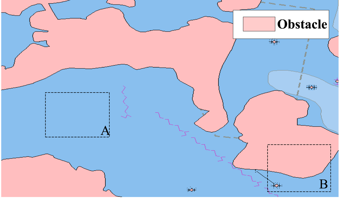
Figure 10. Obstacles extracted from a single chart.

Figure 11. Obstacles fused with multiple charts.

Table 1. Charts relevant to the experimental area

As shown in Figures 10 and 11, the small-scale chart used in the binary tree for generating the navigation route has a large amount of cartographic synthesis of all the elements in the chart due to the limitation of the load carrying capacity of the map, and it is inexact. Take the sea area shown in the dotted line box A as an example. Some actually existing obstacle areas on the small-scale chart are not shown in the figure, which would threaten the navigational safety of the ship. In the dotted line box B on the left of the sea area, there is a situation in which the route is blocked in the navigation area after the cartographic synthesis is completed, and the generated route is no longer the actual shortest route.

Compared with the existing method, the proposed method is more detailed in its construction and expression of the obstacles, as shown in Figure 11. This is because the proposed algorithm not only accurately represents the actual obstruction area (as shown in the area A in Figure 11) by data fusion of the sea areas established from different scale charts but also shows the navigable waterway in usable detail (shown as area B in Figure 11).

4.2. Comparison and analysis of routes generated by different algorithms

Next, the existing route binary tree method and the method proposed in this paper are further compared and analysed for route generation. Two sets of electronic chart data are selected as shown in Table 2 and using the above two methods to plan the route, the test results are shown in Figures 12 and 13. For the ease of comparison, a partial area C of Figure 13 is enlarged and displayed in Figure 14.

Figure 12. Comparison of routes generated by the different methods (Experiment No. 1).

Figure 13. Comparison of routes generated by the different methods (Experiment No. 2).

Figure 14. Route in area C.

Table 2. Relevant charts for generating routes

From the test results shown in Figures 12 and 13, when compared with the existing route binary tree algorithm, the distance of the route generated by the proposed method is obviously shorter than that of the existing algorithm. The proposed method is able to plan the shortest distance route based on the presentation of a finer obstacle course to make full use of the navigable space.

As further shown in Figure 14, which is an enlarged view of area C in Figure 13, the route, which is generated by the existing binary tree algorithm using the small-scale chart, goes across the obstacle area in the large-scale chart. This has the potential to hide dangers to navigation safety.

Generally, the results of the experiment show that compared with the existing route binary tree algorithm, the shortest distance route generated by the method proposed in this paper has been greatly improved both in distance and in safety. The feasibility and reliability of this route can be concluded as shown in Table 3.

Table 3. Comparison of feasibility and reliability

4.3. Comparison and analysis of efficiencies of different algorithms

The difference in the efficiency between the existing route binary tree algorithm and the proposed method is further compared and analysed. The two groups of the shortest distance routes are selected as shown in Figure 11, the basic parameters of the PC used for the test are shown in Table 4, and the efficiency of the test results are shown in Table 5.

Table 4. Hardware configuration for the test

Table 5. Comparison of efficiency

As seen from Table 5, when compared with the existing route binary tree algorithm, the method proposed in this paper significantly shortens the route generation time. This is due to the effective screening of the obstacle course data in the route window, the improvement of the R-tree index and the efficient spatial query of the obstacle course data. Hence, the efficiency is improved.