


I. INTRODUCTION
Tooth enamel constitutes the densest mineralized tissue in the human body. As the outermost layer of the dentition, enamel must endure the mechanically and chemically demanding environment of the oral cavity to enable effective mastication throughout an individual's life. Furthermore, as an acellular tissue, enamel can only be repaired via remineralization from saliva, limiting the body's ability to address tissue damage or loss. To meet these demands, enamel has evolved a multiscale hierarchical structure that achieves high hardness while retaining toughness (He and Swain, Reference He and Swain2007).
Compositionally, mature enamel consists of 95% hydroxyapatite (OHAp), ~1% water, and 4% residual biomacromolecules by weight. The mineral phase exists primarily as high aspect ratio crystallites extended along their crystallographic c-axis with approximately 20 nm × 40 nm rhombohedral cross sections in the basal plane. At the micrometer scale, a tessellating pattern of parallel “enamel rods” with keyhole-shaped cross sections runs from the dentinoenamel junction (DEJ) to the external enamel surface (EES) of the tooth (Figure 1) (Nanci, Reference Nanci2012). Each enamel rod contains ~104 roughly aligned OHAp crystallites. At the center of the rod (“head”), the crystallites’ c-axes are parallel to the long axis of the rod [Figure 1(b), white arrows]; toward the rod boundaries and in the rod “tail”, the c-axes rotate significantly and take a wider range of orientations (Poole and Brooks, Reference Poole and Brooks1961; Meckel et al., Reference Meckel, Griebstein and Neal1965). These boundary regions are termed as “interrod” enamel, and while they are also primarily composed of OHAp crystallites, their density and crystallographic order is comparatively lower than in the rod centers (Nanci, Reference Nanci2012).

Figure 1. (Color online) Structural schemas of tooth enamel. (a) Mesial–distal cross section of human premolar. (b) Isometric view of enamel microstructure adapted from Meckel et al. (Reference Meckel, Griebstein and Neal1965). Keyhole-shaped enamel rods run from DEJ to EES. Overlaid white arrows indicate the putative c-axis orientation of OHAp crystallites comprising each rod. Red highlight in (a) corresponds to the red face of (b) (orientation conserved). (c) Enlarged schematic of enamel in cross section highlighting the approximate dimensions of the disordered interrod regions separating each rod.
Many aspects of this structure have been extensively characterized by a combination of optical microscopy, electron microscopy, and X-ray diffraction. The general dimensions of the rod cross sections and packing have been observed optically in enamel sections in which the interrod regions have been preferentially etched (Boyde, Reference Boyde, Cohen and Kramer1976). Furthermore, polarized light microscopy of thin enamel sections has revealed the divergence of the c-axes as one moves to the rod boundaries (Poole and Brooks, Reference Poole and Brooks1961). The approximate dimensions of both the rod and crystallite cross sections can be determined through scanning electron microscopy (SEM) (Boyde, Reference Boyde1967, Reference Boyde, Cohen and Kramer1976; Habelitz, Reference Habelitz2015) and transmission electron microscopy (TEM) (Kerebel et al., Reference Kerebel, Daculsi and Kerebel1979; Yanagisawa and Miake, Reference Yanagisawa and Miake2003). X-ray diffraction has been used to establish the crystalline phase of enamel, extract lattice parameters, map bulk crystallographic orientation, and approximate crystalline domain size (Glas, Reference Glas1962; Al-Jawad et al., Reference Al-Jawad, Steuwer, Kilcoyne, Shore, Cywinski and Wood2007, Reference Al-Jawad, Addison, Khan, James and Hendriksz2012; Simmons et al., Reference Simmons, Al-Jawad, Kilcoyne and Wood2011; Xue et al., Reference Xue, Zavgorodniy, Kennedy, Swain and Li2013; Al-Mosawi et al., Reference Al-Mosawi, Davis, Bushby, Montgomery, Beaumont and Al-Jawad2018). These and many other studies serve to form the current model of human enamel, as illustrated in Figure 1.
While the literature characterizing enamel's ultrastructure is vast, existing studies face limitations that have prevented a definitive characterization of crystallite populations at the sub-rod length scale. Individual crystallite dimensions can be measured with great accuracy using TEM, and crystallographic orientation can be determined on these same crystallites, but TEM studies suffer from a limited field of view that makes the extraction of population-level statistics impractical. Lower resolution techniques (optical and SEM) can image a large area containing numerous enamel rods but generally require acid etching that disturbs the natural state of the enamel and introduces topography that confounds precise measurements of crystallite dimensions and orientations. X-ray diffraction has the potential to provide population-scale sampling without significantly disturbing enamel's natural state, but in all existing studies, the scale of the X-ray probe has resulted in measurements that average over multiple enamel rods and extensive interrod regions, eliminating the ability to resolve differences across or between individual rods. Because of these challenges, there is currently no clear picture of sub-rod length scale variation of crystallite populations’ dimensions and crystallographic characteristics, i.e., lattice parameters, crystallographic orientations distribution, coherent domain size, and micro-strain.
Here, we introduce a synchrotron microdiffraction approach through which these challenges can be overcome, taking advantage of the strengths of X-ray diffraction (high sampling in a near native state) while still achieving the spatial resolution necessary to independently sample different crystallite populations across individual rods. By machining a 1-μm-thick plate of enamel and performing diffraction with a focused (~500 nm wide) monochromatic X-ray probe, crystallites from only a single rod are sampled at any one position. With lateral specimen dimensions of 18 μm × 8 μm and the expected dimensions for each enamel rod (Figure 1), at least one whole rod cross section is expected in the sample as well as portions from approximately six others. With lateral translational step sizes of 500 nm in both dimensions, each enamel rod can be sampled by 100–200 non-overlapping volumes each of which contains on the order of 300 crystallites.
In order to compare measured quantities from rod vs. interrod populations of crystallites, it is first necessary to identify the boundaries between rods. We chose to do this directly from the X-ray diffraction patterns themselves. Prior work has shown that the crystallographic c-axes of rods in the interrod volumes are much less parallel than in the rod centers (Meckel et al., Reference Meckel, Griebstein and Neal1965). One expects that this would be reflected in transmission X-ray diffraction patterns recorded on an area detector positioned normal to the incident beam, specifically in the azimuthal distribution of intensity around diffraction rings. We herein report the development of a computational method that quantifies the azimuthal autocorrelation of diffracted intensity in specific reflections to compute a metric for crystallographic order/disorder. When applied to a diffraction map taken through a tooth enamel specimen (18 μm × 8 μm × 1 μm dimensions), the method allows for the correlation of crystallographic quantities extracted from each pattern with the enamel microstructure, providing, for the first time, population-specific characterization of rod vs. interrod enamel.
II. EXPERIMENTAL
A deidentified healthy human premolar extracted for orthodontic reasons was obtained from Drs. Akers, Stohle, and Borden of The Center for Oral, Maxillofacial, and Implant Surgery (Evanston, IL) and disinfected in 10% buffered formalin for 10 days. After embedding in epoxy (Epofix 301), a mesial–distal cross section was exposed by cutting with a low-speed Isomet saw (Buehler) using a diamond blade [section illustrated in Figure 1(a)]. The cut surface was then ground and polished to a final roughness of 50 nm, beginning with SiC (600, 800, and 1200) grit paper (Buehler), progressing through aqueous diamond suspensions (6, 3, and 1 μm), and finishing with an alumina suspension (0.05 μm). After sputter coating with 20 nm of Pt for conductance, a Helios dual-beam focused ion beam (FIB) and SEM (FEI) equipped with a tungsten micromanipulator (Omniprobe) was used to extract a thin plate (20 μm × 8 μm × 3 μm) of outer enamel through established liftout procedures described previously (Gordon et al., Reference Gordon, Cohen, MacRenaris, Pasteris, Seda and Joester2015). The resulting section was welded to a copper TEM half-grid (Ted Pella) and thinned to 1 μm. The orientation of the liftout was prepared such that the long axis of the enamel rods runs normal to the largest face of the section [see schemas in Figures 1(b) and 2(a)] and parallel to the eventual X-ray beam direction [Figure 2(c)]. After low-energy 2 kV cleaning of the section surfaces with the ion beam, the TEM half-grid was glued with clear nail varnish to an aluminum bar (~3 cm in length) for ease of handling.
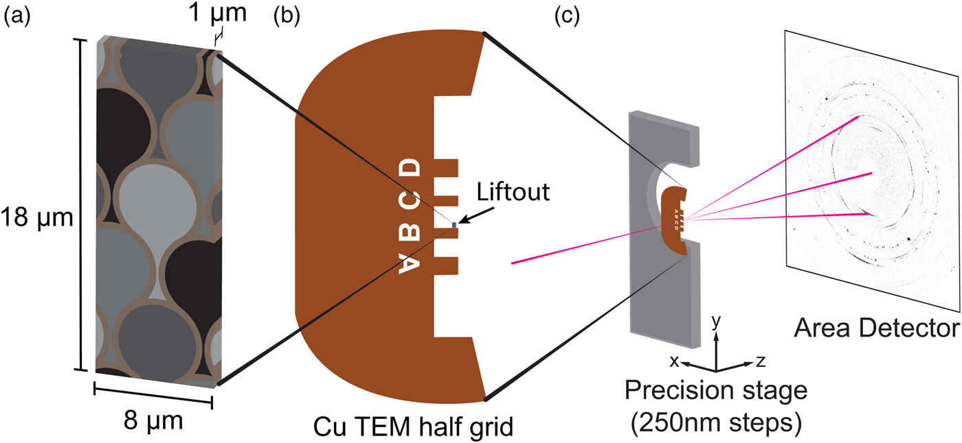
Figure 2. (Color online) Sample geometry and mounting. (a) Schematic of the enamel section after liftout and thinning. Keyhole pattern of enamel rods rendered approximately to scale. (b) Schematic of copper TEM half-grid with the enamel section mounted to post B. (c) Enamel sample positioned at the focal point of the 17 keV X-ray probe to collect 2D diffraction patterns in transmission.
Synchrotron X-ray microdiffraction was performed at beamline 34 ID-E of the Advanced Photon Source (APS) at Argonne National Laboratory (Argonne, IL, USA). Monochromatic X-rays (17 keV) were focused to a probe size of 500 nm × 500 nm, and 2D diffraction patterns were collected in transmission on a MAR165 area detector [Figure 2(c)]. The sample was mounted on a translational stage with 250 nm precision in x, y, and z motions and positioned at the focal point of the beam. Diffraction patterns were collected with two 30 s integrations and correlated to remove spurious counts from gamma rays, yielding an effective exposure time of 60 s per pattern. A 2D map with 500 nm isotropic steps consisting of 943 (23 × 41) patterns was collected across the enamel section, including patterns through air, FIB platinum used for sample mounting, and the copper grid. A calibration pattern was also collected using a powdered ceria (CeO2) standard (NIST).
III. DATA ANALYSIS
Each raw 2D pattern is stored as a 2048 × 2048 16-bit TIFF. To remove signals in the patterns not originating within the enamel sample, 40 patterns collected through air were averaged, and this average was subtracted from each sample pattern using ImageJ (Schneider et al., Reference Schneider, Rasband and Eliceiri2012). Using the 2D Powder Diffraction module of Fit2D, the ceria standard pattern was fit to determine the pixel position of the beam center, sample-to-detector distance, and detector tilt (Hammersley et al., Reference Hammersley, Svensson and Thompson1994). The background-corrected patterns were then transformed from polar to Cartesian coordinates (azimuthal angle χ vs. d-spacing) based on these calibration values [Figures 3(a) and 3(b), top] (Hammersley et al., Reference Hammersley, Svensson, Hanfland, Fitch and Hausermann1996). With the data in this form, integration over all azimuthal angles yields the 1D powder diffraction pattern [Figure 3(b), bottom], and integration over small ranges of d-spacing around specific diffraction peaks yields profiles of intensity vs. azimuthal angle, χ [Figure 3(c)].

Figure 3. (Color online) Data processing and extraction. (a) A single background-corrected 2D diffraction pattern of human enamel. Darker grays indicate higher intensity. (b, top) Cartesian transform of the diffraction pattern in panel (a) plotted as azimuthal angle (χ) vs. d-spacing (Å). (b, bottom) Corresponding 1D diffraction pattern generated by integrating over 360° azimuthally. Indexed peaks for the hydroxyapatite structure. Starred peaks correspond to erroneous scattering not originating in the sample. (c) Intensity vs. azimuthal angle for selected families of reflections within the HA quadruplet: 022 (purple), 030 (yellow), 112 (red), and 121 (blue).
Previous SEM and TEM studies of enamel suggest that the crystallographic order (texture) within the rods is stronger than in the disordered interrod regions (Nanci, Reference Nanci2012). Before describing the method for differentiation rod and interrod materials based on azimuthal distribution of diffracted intensity, it is helpful to review what this distribution represents. Within the irradiated volume of the specimen, a small fraction of the crystallites will be oriented for hkl diffraction. Each of these Bragg-oriented crystallites contributes intensity to a specific small sector or azimuthal bin of the hkl diffraction ring, and the orientation of the hkl normal for that crystallite relative to the laboratory coordinate system defines which bin of the ring receives the increment of diffracted intensity. High intensities at certain azimuths of a ring, therefore, represent orientations heavily populated by crystallites.
An automated computational approach relying upon this difference in texture was developed to identify the boundaries between enamel rods and to classify regions as rod vs. interrod enamel. This quantitative method is based on the azimuthal autocorrelation of diffracted intensity within diffraction ring hkl, I hkl(χ). The azimuthal autocorrelation, r j, of lag j relates the intensities within each azimuthal bin with those that are j azimuthal bins away over the entire profile's domain. r j is defined as
 $$r_j = \displaystyle{{c_j} \over {c_0}}$$
where
 $$c_j = \displaystyle{1 \over L}\sum\limits_{i = 1}^{L-j} {\lpar {I_{ij}-\bar{I}} \rpar \lpar {I_{i + j}-\bar{I}} \rpar }$$
L is the total number of azimuthal bins,  $\bar{I}$ is the mean profile intensity, and c 0 reduces to the sample variance. r j can vary between −1 and 1. In practice, the extracted azimuthal intensity profiles for each reflection initially consist of 2048 angular bins of 0.176° each. Profiles are down-sampled by a factor of 8, yielding L = 256 bins of ~1.4° each. To extract a single quantity that captures the autocorrelation in highly localized neighborhoods, the average autocorrelation of the first 8 lags is defined as the “local azimuthal autocorrelation”,
  $\bar{r}$ (LAA). This averaging also insulates the approach against artifacts introduced by the selection of azimuthal bin size. Pure powder patterns are expected to have a uniform azimuthal distribution of diffracted intensity, resulting in a low LAA, while patterns with high crystallographic texture should have localized intensity, resulting in an increased LAA. Manual observations of 2D diffraction patterns of enamel suggested that the 022, 030, 112, and 121 quadruplet reflections hold texture information [Figure 3(c)], so a final quantity, termed the “combined local azimuthal autocorrelation” (CLAA), was defined as the sum of LAA values for each reflection weighted by their total intensity. This data processing was accomplished with a custom MATLAB (MathWorks 2018b) code.
IV. RESULTS AND DISCUSSION
A series of azimuthal intensity distributions based on various idealized arrangements of crystallites in nanocrystalline materials were examined using the autocorrelation analysis code. The results for the first 50 lags are shown in Figure 4, including the approximate confidence bounds within which no significant correlation exists (assuming Ihkl follows a moving average model). For the case of an ideal powder sample with a uniform orientational distribution and a practically infinite number of crystallites sampled (or the noise only case) [Figure 4(a)], one can see that the autocorrelation falls below the confidence bounds immediately. For an irradiated volume containing aligned crystallites with a wide [Figure 4(b)] or narrow [Figure 4(c)] distribution of orientations, the azimuthal intensity distribution will contain a single Gaussian peak [Figures 4(b) and 4(c)]. In these cases, the autocorrelation at low j values is quite high, and the range of lags over which the autocorrelation remains significant decreases as the peak narrows. In the highly unlikely case in which the irradiated volume contains numerous tightly oriented crystallite populations with very specific angular relations defined by the crystallography of the material, the azimuthal intensity could be periodic in nature [Figure 4(d)]. In this case, one can observe how the autocorrelation at low j values falls off quickly, but the periodicity in azimuthal space results in a reemergence within the autocorrelation plot, reflecting this periodicity in what is effectively frequency space. If the crystallites in the irradiated volume are randomly oriented but relatively finite in number (in contrast to the ideal powder of case a), the periodicity in the azimuthal intensity plot is destroyed and peaks are randomly distributed [Figure 4(e)], the autocorrelation once again falls below the confidence bounds very quickly, and no later peaks in the autocorrelation plots are observed. Finally, if the irradiated volume contains multiple orientations of tightly aligned crystallites, the azimuthal intensity distribution will appear as peaks randomly distributed around separated loci [Figure 4(f)]. The autocorrelation plot in this case mirrors that of a single Gaussian peak but with slightly reduced low j values.

Figure 4. (Color online) Examples of azimuthal autocorrelation. The left column plots simulated azimuthal intensity profiles of (a) uniform distribution (or noise only), (b) a single broad peak, (c) a single sharper peak, (d) 18 sharp, evenly spaced peaks, (e) 36 sharp, randomly distributed peaks, and (f) 72 sharp, peaks clustered randomly about 3 evenly spaced loci. Peaks are Gaussian, and the total integrated intensity of each profile is conserved (5000 cts) between cases. Poisson noise with a mean of 30 cts was added to each profile. Colored plots are down-sampled by a factor of 8 from the raw simulated profiles, which are provided as grayscale inlays beneath each plot. The right column plots the azimuthal autocorrelation for the first 50 lags (1.4° bins) corresponding to each profile on the left, effectively capturing the autocorrelation localized to 70° neighborhoods within each profile. For each case, the light gray dotted lines indicate the approximate confidence bounds within which no significant correlation exists (assuming Ihkl follows a moving average model). The LAA is taken as the average autocorrelation value ( $\bar{{r}}$) for the first 8 lags (starred bracket, bottom right plot), and these values are provided beneath each plot.
Comparing the LAA ( $\bar{r}$) values between these simulated patterns (Figure 4, right plot) reveals a few notable features of the metric that are relevant to interpreting
  $\bar{r}$ values extracted from experimental patterns. First,
  $\bar{r}$ represents the autocorrelation between only localized azimuthal neighborhoods (<12°). As a result, even patterns with differing long-range autocorrelations like cases a, d, and e can result in similar
  $\bar{r}$ values. Meanwhile,
  $\bar{r}$ is also composed of r j values that are computed by sums over the entire azimuthal intensity distribution (see definition above), so
  $\bar{r}$ captures the local autocorrelation across the entire 360° azimuthal domain. Comparing cases b and c illustrates one result of this aspect of the LAA metric; the larger peak breadth in case b corresponds to a larger number of sum terms contributing a strong positive autocorrelation, and thus, the LAA is larger than in case c. This highlights an important caveat of applying the LAA metric: for smoothly varying, well-defined azimuthal intensity peaks, a higher value of
  $\bar{r}$ generally corresponds to a broader peak, and thus implies a less ordered distribution of crystallites. However, profiles of this type are generated in cases where the number of diffracting crystallites is practically infinite, i.e., the individual crystallite volume is many orders of magnitude smaller than the irradiated volume. In such cases, texture can be easily quantified through more direct approaches, e.g., fitting the azimuthal distribution with a Gaussian and using the peak-width as a metric for texture. The utility of the LAA metric emerges when seeking to quantify the order/disorder within more complex azimuthal intensity distributions, especially those generated when the number of diffracting crystallites is finite. Cases e (disordered) and f (ordered) exemplify two such scenarios, and comparing the LAA values, 0.07 and 0.63, respectively, illustrates how
  $\bar{r}$ can quantify the differences in order where traditional peak fitting approaches would be inadequate.
The measured azimuthal intensity profiles from human enamel appear to vary in their apparent degrees of crystallographic order. Figure 5 details two typical patterns: one showing highly ordered azimuthal intensities (Figure 5, left column) and another showing less ordered azimuthal intensities (Figure 5, right column). Qualitatively, the azimuthal intensity profiles for the ordered pattern [Figure 5(c)] appear very similar to the simulated case of peaks distribute around ordered loci (Figure 4, case f), while those of the disordered pattern [Figure 5(d)] appear much more akin to the case of randomly distributed peaks (Figure 4, case e). None of the profiles correspond well with the smoothly varying Gaussian cases (Figure 4, cases b and c), because the 500 nm beam employed in this study irradiates only a few hundred crystallites, far from the pseudo-infinite condition general sought in powder diffraction experiments. Application of the autocorrelation method produces computed LAA values for the 121 and 030 rings: 0.76 and 0.71, respectively, for the ordered pattern and 0.35 and 0.26, respectively, for the disordered pattern. The LAA is thus able to quantify the differences in order between these two typical patterns.

Figure 5. (Color online) Two archetypical diffraction patterns for human enamel. (a) 2D diffraction pattern from an ordered region. Diffraction spots are concentrated in distinct arcs. (b) 2D diffraction pattern from a disordered region. Diffraction spots are more distributed azimuthally and arcs are not as distinguishable. (c, top) Cartesian transform (d-spacing vs. azimuthal angle) of panel (a) in the region of quadruplet reflections and (c, bottom) azimuthal intensity profiles for the 030 and 121 reflections. (d) Corresponding pattern and profiles for (b). For all diffraction patterns, darker gray indicates higher intensity. (e and f) Azimuthal autocorrelations for the 121 profiles plotted in (c) and (d), respectively. Inset shows first 32 lags and indicates the LAA,  $\bar{r}$, for each case.
Maps of the spatial variation in LAA can be produced for the different reflections (data not shown). Combining the LAA for the 022, 030, 112, and 121 rings produces a map of the combined local azimuthal autocorrelation (CLAA) for the entire enamel section (Figure 6). The characteristic keyhole-shaped pattern of the human enamel microstructure is clearly resolved, with the rod centers having relatively high CLAA values (ordered crystallites), while the tail and interrod regions have relatively low CLAA values (disordered crystallites), consistent with observations of crystallite axes previous detailed (Nanci, Reference Nanci2012). The scale of the features (~5 μm) is also consistent with those expected for enamel rods. These CLAA values can now be used to classify patterns in the map as rod vs. interrod and establish the relative location of the sampled crystallite populations in each pattern within the enamel microstructure.

Figure 6. (Color online) CLAA map of the enamel section. On left, fine map (0.5 μm step size) of the combined autocorrelation of the quadruplet reflections. On right, schema of the enamel microstructure (approximately to scale with map). Keyhole structure of rod cross section is well-resolved by contrast in the local autocorrelation.
The present approach collects data from hundreds of crystallites within each pattern across the enamel microstructure; data which are not complicated by the sampling of multiple rods simultaneously. Earlier X-ray diffraction microbeam determinations of lattice parameters, of crystallite size, and of crystallographic texture averaged over many rods and were intrinsically unsuitable for determining variations within rods (Al-Jawad et al., Reference Al-Jawad, Steuwer, Kilcoyne, Shore, Cywinski and Wood2007). Now, the key aspects of the present approach, namely the small specimen thickness, small probe size (~500 nm), and the development of the LAA metric to accurately localize patterns within the enamel microstructure, enable the crystallite populations of the rod and interrod regions to be separately characterized via X-ray diffraction for the first time. Due to space constraints and a desire to provide a report focused on the LAA as a metric for characterizing nanocrystalline order/disorder, these results are not included here. However, a forthcoming report by the authors will describe how the crystallographic features of human enamel (e.g., lattice parameters, crystallite size, and orientation of crystallites) vary in the context of the rod/interrod microstructure and provide population-level statistics that are impractical to obtain via other methods (e.g., TEM).
These forthcoming crystallite population studies have implications for our understanding of amelogenesis (enamel development), of congenitally defective enamel, of enamel affected by physiological insult during growth, of biomimetic enamel mineralization, and of prophylactic and restorative treatments for the damaged tooth enamel. The approach could be used to compare enamel sub-rod characteristics of modern vs. archeological humans or of members of related clades (extant vs. extinct species) and the extent to which diagenesis has altered structure. The 3D organization of rods differs enormously, for example, in enamel of humans vs. rodents, and it would be interesting to apply this approach to determine if there are variations in crystallite organization as well. Beyond tooth enamel, the use of azimuthal autocorrelation to quantify crystallographic order in large 2D diffraction datasets has value to other nano-grained materials, especially those with multiscale crystallographic complexity.
ACKNOWLEDGMENTS
The authors thank J.D. Almer for sharing pieces of the Sector 1, APS, MATLAB code for transmission diffraction pattern analysis; while not directly employed here, this code base informed and accelerated the development of the novel methods described in this paper.
This research used resources of the Advanced Photon Source, the U.S. Department of Energy (DOE) Office of Science User Facility operated for the DOE Office of Science by Argonne National Laboratory under Contract No. DE-AC02-06CH11357.
FUNDING INFORMATION
Funding for this work comes from the NIH in the form of an RO1 (DE025702-01) and an F31 Fellowship (DE026952). This work made use of Northwestern's MatCI core facility which receives support from the MRSEC Program (NSF DMR- 1720139) of the Materials Research Center at Northwestern University. Sample preparation was also performed at the EPIC core facility which receives support from the Soft and Hybrid Nanotechnology Experimental (SHyNE) Resource (NSF ECCS-1542205); the MRSEC program (NSF DMR-1121262) at the Materials Research Center; the International Institute for Nanotechnology (IIN); and the State of Illinois, through the IIN.


