NOMENCLATURE
- SAK
smart adaptation kit
- GCM
guidance and control module
-
 $$V_{t} $$
free-stream velocity
- L
lift
- W
weight
- T
thrust
- D
drag
- U,V,W
linear velocity components along body x-, y, and z-axis
-
$$C_{L} ,C_{D} ,C_{Y} $$
coefficient of lift, drag and side force
- l,m,n
components of the aerodynamic moments (roll, pitch and yaw moments) in the body frame
-
$$C_{l} ,C_{m} ,C_{n} $$
roll, pitch and yaw moment coefficients
- m
mass of the vehicle
-
$$\bar{c}$$
mean aerodynamic chord
-
$$S_{{Ref}} $$
reference area
-
$$q_{\infty} $$
free stream dynamic pressure
- LCF,RCF
left and right control fins
-
$$J_{x} ,J_{y} ,J_{z} ,J_{{xz}} $$
components of the inertia matrix in body frame
-
$$X_{A} ,Y_{A} ,Z_{A} $$
components of the aerodynamic force (axial, side and tangential force) in the body frame
-
$$P_{e} ,P_{n} $$
position co-ordinates along the inertial east and north directions
- g
acceleration due to gravity
- p, q, r
roll, pitch and yaw rates are the angular velocity components in the body frame
- h
altitude
- km
kilometer


Greek symbol
-
$${\rm \rrho }$$
density of the air
-
$${\rm \ralpha }$$
aerodynamic angle-of-attack
-
$$\rphi ,{\rm \rtheta },{\rm \rpsi }$$
Euler angles (roll, pitch and azimuth angles) defining body frame w.r.t. inertial frame
-
$${\rm \rgamma }$$
flight path angle
-
$${\rm \rbeta }$$
side slip angle


1.0 INTRODUCTION
The conventional aerial munitions such as general purpose bombs, penetration bombs and practice bombs are widely utilised across the globe and constitute a major portion of the weapon arsenal of different countries( Reference Ressler and Wise 1 ). These munitions instead of following a ballistic trajectory towards the designated target, merely follows a free-fall trajectory. This results in limited range (typically around 15 km) and accuracy of the munition. In addition to this, an intrinsic problem associated with the use of these munitions is that the launching aircraft has to come close to the target. This exposes the launching platform to enemy's surface-to-air missiles and guns.
The effective utilisation of these munitions depends on various factors such as launching platform capabilities, pilot skills, environmental conditions and target area. Therefore, a multifaceted problem of mission complexity and aircraft survivability behind enemy lines is encountered. In order to reduce such risks, requirement exists for utilisation of smart munitions with extended range and high accuracy. High existing stockpile of such traditional munitions in the countries military systems imposes a financial restriction for shifting to smart munition. Therefore, instead of exposing to an altogether new technology which is based on smart weapons, efforts have been made to develop an interface mechanism which can transform the available general purpose munition into smart munition. To achieve this objective, various interface kits such as but not limited to JDAM & JDAM-ER ( Reference Anderson and Teope 2 , Reference USAFR 3 ), GBU-15 ( Reference Lee 4 ) and Griffin ( Reference Singh 5 ) have been developed and utilised by different countries. These modification kits convert the short-range unguided aerial munitions( Reference Rigby 6 ) into fairly accurate medium range guided munitions. Utilisation of such interfaces enabled the aircraft to launch weapons from considerably far distance which reduced the chances of aircraft vulnerability.
The use of global positioning system (GPS) is very common in such interface kits( Reference Wise, Lavretsky, Zimmerman, Francis, Dixon and Whitehead 7 ). GPS provides considerable accurate navigation data for precise tracking of the inertial trajectories. However, traditional guidance and control architectures used to guide the vehicle along such trajectories proved inadequate in situations where frequent heading changes were required. Such systems are designed separately using well-established control strategies, such as Line of Sight (LOS) for guidance. Reference 8 contains interesting application to the air carriers. During the design phase, the control system is usually designed with sufficiently large bandwidth to track the commands that are expected from the guidance system. However, because the two systems are effectively coupled, stability and adequate performance of the combined system about nominal trajectories are not guaranteed. In a real-world scenario, this problem can be resolved by judicious choice of guidance law parameters (such as the visibility distance in LOS strategy), based on extensive computer simulations. Even when stability is obtained, the resulting strategy leads to finite trajectory tracking errors. The relative error of which depends on the type of trajectory to be tracked (radius of curvature, vehicle speed and so on). Due to the same reasons, considerable errors exist in the tracking of ground targets, by the aerial platform.
The subject of trajectory tracking has also been addressed in the literature for the control of non-holonomic vehicles. In Ref. 9, an interesting case of tracking a nominal trajectory by a non-linear system is discussed. The paper includes examples of applications of the proposed technique to different systems. The nominal trajectories considered in Ref. 9 are not restricted to be trimming trajectories. Another approach is used in Ref. 10, where a tracking problem for a surface marine vessel is considered. Here the authors use feedback linearisation with dynamic extension to obtain a controller to track trajectories that consist of lines and arcs of circles (a special case of trimming trajectories in the plane). The solution of the trajectory tracking problem proposed in this paper differs from Refs 9 and 10. In this paper, the key idea is to reduce the problem to the design of a tracking controller for a linear time-invariant system utilising much simpler architecture for the vehicle kinematics. In the linear setting, the designer is free to choose his favourite control synthesis technique to achieve the desired closed-loop performance and robustness.
To improve the overall performance of aerial munitions, integrated guidance and control design method has been developed utilising various control techniques. Wise( Reference Wise, Lavretsky, Zimmerman, Francis, Dixon and Whitehead 7 ) proposed direct adaptive model reference control to a modified MK-82 Joint Direct Attack Munition weapon flight control system. The adaptive flight control augments the weapon's baseline autopilot which was designed using a linear quadratic regulator (LQR) incorporating integral control. While the latter was constructed to provide system stability and command tracking using nominal plant data, the adaptive augmentation was designed to maintain the desired closed loop system characteristics in the presence of the aerodynamic uncertainties. Kim et al.( Reference Kim and Grider 11 ) proposed terminal guidance of re-entry vehicles with constrained attitude angle at impact by applying linear quadratic optimisation techniques. The guidance system with time-varying feedback gains was shown to meet the given specifications for a certain region of initial states. Ratnoo et al.( Reference Ratnoo and Ghose 12 ) proposed a proportional navigation-based guidance law for a non-stationary and non-manoeuvring target with impact angle constraint. Ryoo et al.( Reference Ryoo, Cho and Tahk 13 ) proposed a generalised formulation of energy minimisation optimal guidance law with impact angle constraint for a constant speed missile with an arbitrary order.
Harl et al.( Reference Harl and Balakrishnan 14 ) proposed an approach to impact time and angle guidance for a missile utilising a combination of line-of-sight rate shaping technique and a second-order sliding mode control. Due to the robustness of the control law, the proposed methodology could be applied to many realistic engagement scenarios including uncertainties such as a moving target. Similarly, Hou et al.( Reference Yang, Guo and Zhou 15 ) utilised a combination of non-linear extended disturbance observer and sliding mode control techniques to design the integrated guidance and control law for homing missiles against ground-fixed targets. Vaddi( Reference Vaddi, Menon and Ohlmeyer 16 ) used the numerical state-dependent Riccati equation technique with a more comprehensive model characterised by non-linear motion in the dimensions. Reference 17 used the feedback linearisation law associated with the LQR technique to formulate a non-linear integrated guidance and control law for homing missile. In Ref. 18, a linear quadratic differential game-type guidance law was derived for a dual controlled missile. Ref. 19 designed an integrated guidance and control law by using sliding mode control methodology; Ref.(20) used subspace stabilisation method to formulate a non-linear integrated guidance and control law for homing missile.
Han et al.(
Reference Han, Zheng and Chong
21
) proposed an integrated guidance and control technique to engage a ground-fixed target by a guided bomb using the
 $${\rm \rtheta }{\minus}D$$
method. First, the basic longitudinal mathematical integrated guidance and control model was established, and then
$${\rm \rtheta }{\minus}D$$
method. First, the basic longitudinal mathematical integrated guidance and control model was established, and then
 $${\rm \rtheta }{\minus}D$$
methodology was employed to obtain an approximate closed form solution to this integrated guidance and control problem based on approximations to the Hamilton–Jacobi–Bellman equation. The performance of designed algorithm was then validated through numerical simulations. In another study, Kim et al.(
Reference Kim, Kim and Park
22
) designed guidance and control system to impact a target with a desired impact angle for precision guided bombs such as JDAM. The guidance and control system architecture was composed of autopilot loop and impact angle control guidance loop. The impact angle control guidance was achieved utilising linear quadratic optimal control technique. And non-linear 6-degree of freedom (DOF) simulations are carried out to examine the performance of the closed loop system.
$${\rm \rtheta }{\minus}D$$
methodology was employed to obtain an approximate closed form solution to this integrated guidance and control problem based on approximations to the Hamilton–Jacobi–Bellman equation. The performance of designed algorithm was then validated through numerical simulations. In another study, Kim et al.(
Reference Kim, Kim and Park
22
) designed guidance and control system to impact a target with a desired impact angle for precision guided bombs such as JDAM. The guidance and control system architecture was composed of autopilot loop and impact angle control guidance loop. The impact angle control guidance was achieved utilising linear quadratic optimal control technique. And non-linear 6-degree of freedom (DOF) simulations are carried out to examine the performance of the closed loop system.
In this paper, an innovative approach for the design of a guidance and control system is presented that can alter the flight path of the free fall projectile from the standard ballistic trajectory. This results in enhanced ranges and high precision for engaging the target. We explain from the very beginning the entire design cycle of the guidance and control. This includes the fundamentals for the design of (a) adaptation kit, (b) stability controller, (c) a method for determining the angular orientation estimation and (d) guidance law for the vehicle without thrust.
The aerodynamic model utilised in this research is based on the six degree of freedom (6-DOF) dynamic model ( Reference Masud, Chughtai and Akhtar 23 , Reference Sargar, Agrawal and Mohandaas 24 ). Using the concepts outlined in Ref. 25, the orientation of the aerial vehicle is given in terms of its location with respect to the closest point on the desired optimal trajectory. Tracking of a reference trajectory by the vehicle at a certain speed is then converted into the problem of driving a generalised error vector, which implicitly includes the orientation and distance to the desired trajectory. It is noticeably mentioned that the linearisation of the generalised error dynamics about the corresponding trimming path is time invariant. Using these results, the problem of trajectory tracking is posed and solved in the framework of gain scheduled control theory. Simple algorithm for implementing the linear controller for the non-linear system is formulated, such that the properties of linear controller are preserved along each trajectory. This is in contrast to the approach in Ref. 9, where the problem is reduced to designing an exponentially stable state-feedback controller for a linear time-varying system. This leads to a controller design that is problem-specific and does not address the issues of performance and robustness. Numerical simulation showed the effectiveness of the designed architecture as considerable enhancement in range apart from improved CEP was achieved. Although the research work presented promising results, the study needs further hardware implementation through flight demonstration.
1.1 Main contributions of this paper
1. Development of an original SAK: In this research, an original SAK is developed, which transforms the free-fall aerial munition into a smart munition. The SAK contains (i) an adaptation mechanism to carry the munition; (ii) pop-out wings, that allow SAK to glide towards the target; (iii) a pair of control fins, for roll and directional movements; and (iv) a GCM, for guidance and control. The proposed framework for the development of SAK is explained in detail in Section 2.1.
2. Development of guidance and control module (GCM): In order to convert the free-fall munition into a smart munition, requirement exists that the munition follows an optimised ballistic trajectory in the three-dimensional space. To achieve this goal, the on-board GCM is equipped with three fundamental modules namely (1) actuator dynamics module, (2) vehicle dynamics module and (3) controller dynamics module. The controller dynamics module contains (a) a scheduler, for gain scheduling; (b) a guidance controller, for computing guidance/inertial reference trajectory data and providing estimates for the vehicle's attitude and orientation; and (c) a stabilisation controller, to generate the actuator signals that are required to drive the actual velocity and attitude of the vehicle to the values commanded by the guidance scheme. This paper proposes an open methodology for an original SAK, whereby both the guidance and control systems are designed simultaneously, as explained in Section 4.
3. Extended ballistic range and accuracy: Utilising the proposed algorithm, the munition free-fall ballistic range of 15 km is extended in simulations to ranges comparable with what is achieved through the majority of existing modification kits, e.g. but not limited to Refs 2 and 3. Apart from this, considerable improvement in accuracy is achieved with improved CEP.
4. Open architecture and cost-effective solution: This research presents an open architecture and cost-effective frame work with non-propriety information.
The investigations made in this research provided a mathematical-based analysis for designing a preliminary guidance and control system for converting a free-fall munition into a smart munition. Although the theoretical validation of the proposed architecture was made through extensive simulations, the suggested model needs further hardware implementation and validation through flight demonstration.
1.2 Organisation of the paper
The paper is organised as follows. Section 2 discusses the geometrical and design parameters of the SAK. Rigid body dynamics utilising 6-DOF model( Reference Stevens, Lewis and Johnson 26 ) are then discussed. The aerodynamic forces and moments throughout the flight regime are evaluated utilising empirical and non-empirical techniques (USAF Stability and Control( Reference Finck 27 ) and computational fluid dynamics (CFD)( Reference Buning, Gomez and Scallion 28 , Reference Petterson 29 )). In Section 3, optimal ballistic trajectories are determined for various flight conditions. The problem is configured as an optimal control problem to utilise the well-established tools of optimal control. Results from dynamical systems’ theory are applied to investigate local stability characteristics of SAK around the steady-state points. Dynamic characteristics of the open-loop configuration are assessed to generate adequate benchmark performance for closed-loop controller design. Section 4 presents the control law synthesis. The control architecture utilises LQR controller for closed loop stability. Important aspects of the control architecture are discussed. Simulation results depicted the munition glide range enhancement to about 100 km; however, the problem of navigation was encountered. Guidance controller is then added in the closed loop system to minimise the tracking error and to ensure the munition movement towards the target direction. Section 5 concludes the paper.
2.0 PROBLEM SETUP
2.1 Smart adaptation kit (SAK) model
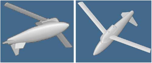
The SAK developed in this study consists of a central main body to which the aerial munition is attached. The SAK itself is attached to the belly of the aircraft via a bolting mechanism. Upon release from the aircraft, SAK wings pop-out from their initial folded position to the fully extended position. This enables the SAK to glide towards the target. The geometrical view of the designed SAK obtained through USAF Datcom( Reference Finck 27 ) is depicted in Fig. 1.
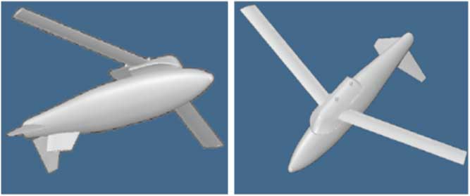
Figure 1 SAK used in this research.
The GCM developed for the SAK provides real-time guidance commands to achieve stabilisation and directional control. To reduce the cost of the modification kit, the number of control surfaces has been kept to a bare minimum. Utilising a single pair of control fins located at the rear end of the fuselage, both the roll and yaw movements are controlled. Like ailerons, these control surfaces can be asymmetrically deflected to control the roll movement. For directional control, they can be symmetrically deflected similar to the rudder functions. This modification resulted in a highly non-linear coupled motion of the vehicle in response to control surface deflection. This design, therefore, made the control architecture more challenging. The dedicated GCM designed for the SAK constitutes (a) a scheduler, for near real-time trajectory generation; (b) a stability controller, for platform stabilisation; and (c) a tracking controller for tracking the optimised trajectory. Presently, 1,000 lb class Mk-82 series free-fall munitions can be retrofit to smart munition through this kit. When the munitions reach the vicinity of the target, the explosive charge is activated by a suitable control permitting SAK to jettison the munition without interference. Complete geometrical description and design parameters of SAK are shown in Table 1.
Table 1 SAK geometric and mass properties
2.2 Flight dynamics model
In order to evaluate performance, as well as to develop a guidance and control system, it has to create a suitable model that meets the specific properties of the guided bomb. In this research, 6-DOF ( Reference Mir, Maqsood and Akhtar 30 ) model which is typically utilised in flight dynamic modelling, is used to model the vehicle motion in the 3D space. A flat Earth approximation is used to define the inertial co-ordinate system. The body frame is defined by the conventional manner. The dynamic equations are written with respect to body co-ordinates with appropriate kinematic equations relating body translational and rotational rates and with inertial translational and Euler angle rotational rates, respectively. The governing equations of motion representing (a) dynamics of translation (Equations (1)), (b) dynamics of rotation (Equations (2)), (c) kinematics (Equations (3)) and (d) navigation (Equation (4)), assuming non-rotating Earth, are defined as
 $$\matrix{ {\dot{U}} \hfill & {{\equals}RV{\minus}QW{\minus}g\sin \rtheta {\plus}{{X_{A} {\plus}X_{T} } \over m}} \hfill \cr {\dot{V}} \hfill & {{\equals}{\minus}RU{\plus}PW{\plus}g\sin \rphi \cos \rtheta {\plus}{{Y_{A} {\plus}Y_{T} } \over m}} \hfill \cr {\dot{U}} \hfill & {{\equals}QU{\minus}PV{\plus}g\cos \rphi \cos \rtheta {\plus}{{Z_{A} {\plus}Z_{T} } \over m}} \hfill \cr {} \hfill & {} \hfill \cr } $$
 $$\matrix{ {\Gamma \dot{P}} \hfill & {{\equals}J_{{XZ}} (J_{X} {\minus}J_{Y} {\plus}J_{Z} )PQ{\minus}[J_{Z} (J_{Z} {\minus}J_{Y} ){\plus}J_{{XZ}}^{2} ]QR{\plus}J_{Z} l{\plus}J_{{XZ}} n} \hfill \cr {\Gamma \dot{Q}} \hfill & {{\equals}(J_{Z} {\minus}J_{X} )PR{\minus}J_{{XZ}} (P^{2} {\minus}R^{2} ){\plus}m} \hfill \cr {\Gamma \dot{P}} \hfill & {{\equals}[J_{X} (J_{X} {\minus}J_{Y} ){\plus}J_{{XZ}}^{2} ]PQ{\minus}J_{{XZ}} (J_{X} {\minus}J_{Y} {\plus}J_{Z} )QR{\plus}J_{{XZ}} l{\plus}J_{X} n} \hfill \cr {} \hfill & {} \hfill \cr } $$
 $$\matrix{ {\dot{\rphi }} \hfill & {{\equals}P{\plus}\tan \rtheta (Q\sin \rphi {\plus}R\cos \rphi )} \hfill \cr {\dot{\rtheta }} \hfill & {{\equals}Q\cos \rphi {\minus}R\sin \rphi } \hfill \cr {\dot{\rpsi }} \hfill & {{\equals}{{Q\sin \rphi {\plus}R\cos \rphi } \over {\cos \rtheta }}} \hfill \cr {} \hfill & {} \hfill \cr } $$
 $$\matrix{ {\dot{P}_{E} } \hfill & {{\equals}U\cos \rtheta \cos \rpsi {\plus}V({\minus}\cos \rphi \sin \rpsi {\plus}\sin \rphi \sin \rtheta \cos \rpsi )} \hfill \cr {} \hfill & {{\plus}W(\sin \rphi \sin \rpsi {\plus}\cos \rphi \sin \rtheta \cos \rpsi )} \hfill \cr {\dot{P}_{N} } \hfill & {{\equals}U\cos \rtheta \sin \rpsi {\plus}V(\cos \rphi \cos \rpsi {\plus}\sin \rphi \sin \rtheta \sin \rpsi )} \hfill \cr {} \hfill & {{\plus}W({\minus}\sin \rphi \cos \rpsi {\plus}\cos \rphi \sin \rtheta \sin \rpsi )} \hfill \cr {\dot{h}} \hfill & {{\equals}U\sin \rtheta {\minus}V\sin \rphi \cos \rtheta {\minus}W\cos \rphi \cos \rtheta } \hfill \cr {} \hfill & {} \hfill \cr } $$
where U, V and W are the linear velocities along body x-, y- and z-axis, respectively,
 $$\rphi ,{\rm \rtheta }\,\,{\rm and}\,\,{\rm \rpsi }$$
are the Euler angles defining the orientation of body frame with respect to inertial frame, P, Q and R are the angular velocities along body x-, y- and z-axis, respectively,
$$\rphi ,{\rm \rtheta }\,\,{\rm and}\,\,{\rm \rpsi }$$
are the Euler angles defining the orientation of body frame with respect to inertial frame, P, Q and R are the angular velocities along body x-, y- and z-axis, respectively,
 $$P_{n} $$
and
$$P_{n} $$
and
 $$P_{e} $$
are the position co-ordinates along the inertial north and east directions, h is the vehicle altitude,
$$P_{e} $$
are the position co-ordinates along the inertial north and east directions, h is the vehicle altitude,
 $$X_{A} ,Y_{A} ,Z_{A} $$
are the axial, side and tangential forces defining components of the aerodynamic force in the body frame, m is the mass, g is the acceleration due to gravity, J is the moment of inertia matrix, l, m and n are the angular velocity components (roll, pitch and yaw moments) in the body axis, α and β are the aerodynamic angles representing angle-of-attack and side slip angle, respectively.
$$X_{A} ,Y_{A} ,Z_{A} $$
are the axial, side and tangential forces defining components of the aerodynamic force in the body frame, m is the mass, g is the acceleration due to gravity, J is the moment of inertia matrix, l, m and n are the angular velocity components (roll, pitch and yaw moments) in the body axis, α and β are the aerodynamic angles representing angle-of-attack and side slip angle, respectively.
2.3 Aerodynamic parameters estimation
The aerodynamic forces and moments acting on the aerial vehicle during different stages of the flight are governed by Equations (5) and (6) respectively:
 $$\matrix{ {L{\equals}q_{\infty} SC_{L} ,D{\equals}q_{\infty} SC_{D} ,Y{\equals}q_{\infty} SC_{Y} } \hfill \cr {} \hfill \cr } $$
where L, D and Y are the aerodynamic lift, drag and side force, respectively, in the wind axis.
 $$q_{\infty} $$
is the dynamic pressure, S is the wing area and
$$q_{\infty} $$
is the dynamic pressure, S is the wing area and
 $$C_{L} ,C_{D} \,{\rm and}\,C_{Y} $$
are the dimensionless aerodynamic coefficients for lift, drag and side forces, respectively:
$$C_{L} ,C_{D} \,{\rm and}\,C_{Y} $$
are the dimensionless aerodynamic coefficients for lift, drag and side forces, respectively:
 $$l_{w} {\equals}q_{\infty} bSC_{l} ,\quad m_{W} {\equals}q_{\infty} cSC_{m} ,\quad n_{W} {\equals}q_{\infty} bSC_{n} $$
where l
w
, m
w
and n
w
are the roll, pitch and yaw moment in the wind axis, respectively, b is the wing span, c is the wing chord and
 $$C_{l} ,C_{m} \,{\rm and}\,C_{n} $$
are the dimensionless aerodynamic coefficients for roll, pitch and yaw moments, respectively.
$$C_{l} ,C_{m} \,{\rm and}\,C_{n} $$
are the dimensionless aerodynamic coefficients for roll, pitch and yaw moments, respectively.
The body aerodynamic force and moment coefficients in Equations (5) and (6) vary with the flight conditions and control settings. A high fidelity aerodynamic model is necessary to accurately determine these aerodynamic coefficients. In this research, both empirical( Reference Roskam 31 ) and non-empirical techniques (such as CFD( Reference Petterson 29 ) and USAF Datcom( Reference Finck 27 )) are utilised to determine these coefficients. The high fidelity model employed for aerodynamic parameter estimation is elaborated in the following equation:
 $$\matrix{ {C_{i} {\equals}C_{{i,{\rm static}}} ({\rm \ralpha ,\rbeta ,\delta }_{{{\rm control}}} ,M){\plus}C_{{i,{\rm dynamic}}} ({\dot{\ralpha }, \dot{\rbeta }},p,q,r)} \hfill \cr {} \hfill \cr } $$
where C i =C L , C D , C Y , C l , C m , C n represent the coefficient of lift, drag, side force, rolling moment, pitch moment and yawing moment, respectively.
The non-dimensional coefficients are usually obtained through linear interpolations using data obtained from various sources. In this research, different methodologies were adopted to ascertain the static and dynamic components of these coefficients(
Reference Le Roy, Morgand and Farcy
32
). Evaluation of static (basic) coefficient data (see Equation (8)) was performed employing CFD(
Reference Buning, Gomez and Scallion
28
,
Reference Petterson
29
) technique. All the parameters were obtained as a function of control (
 $${\rm \delta }_{{{\rm control}}} )$$
, angle-of-attack (α), side slip (β) and Mach number (M)
$${\rm \delta }_{{{\rm control}}} )$$
, angle-of-attack (α), side slip (β) and Mach number (M)
 $$\matrix{ {C_{{i,{\rm static}}} ({\rm \ralpha ,\rbeta ,\delta }_{{{\rm control}}} {\rm ,M})} \hfill & {\Rightarrow C_{{D_{b} }} ({\rm \ralpha ,\rbeta ,\delta }_{{{\rm control}}} {\rm ,M}),C_{{L_{b} }} ({\rm \ralpha ,\rbeta ,\delta }_{{{\rm control}}} {\rm ,M}),C_{{Y_{b} }} ({\rm \ralpha ,\rbeta ,\delta }_{{{\rm control}}} {\rm ,M}),} \hfill \cr {} \hfill & \vskip8pt {C_{{l_{b} }} ({\rm \ralpha ,\rbeta ,\delta }_{{{\rm control}}} {\rm ,M}),C_{{m_{b} }} ({\rm \ralpha ,\rbeta ,\delta }_{{{\rm control}}} {\rm ,M}),C_{{n_{b} }} ({\rm \ralpha ,\rbeta ,\delta }_{{{\rm control}}} {\rm ,M}),} \hfill \cr {} \hfill & {} \hfill \cr } $$
where
 $$C_{{D_{b} }} $$
,
$$C_{{D_{b} }} $$
,
 $$C_{{L_{b} }} $$
,
$$C_{{L_{b} }} $$
,
 $$C_{{Y_{b} }} $$
,
$$C_{{Y_{b} }} $$
,
 $$C_{{l_{b} }} $$
 $$C_{{m_{b} }} $$
and
$$C_{{m_{b} }} $$
and
 $$C_{{n_{b} }} $$
represents the basic components of the aerodynamic forces and moments as a function of (
$$C_{{n_{b} }} $$
represents the basic components of the aerodynamic forces and moments as a function of (
 $${\rm \delta }_{{{\rm control}}} )$$
, angle-of-attack (α), side slip (β) and Mach number (M).
$${\rm \delta }_{{{\rm control}}} )$$
, angle-of-attack (α), side slip (β) and Mach number (M).
Dynamic component (Equation (9)) consists of rate and acceleration derivatives. These are evaluated utilising empirical( Reference Roskam 31 ) and non-empirical ('USAF Stability and Control DATCOM' ( Reference Finck 27 )) techniques:
 $$\matrix{ {C_{{i,{\rm dynamic}}} ({\dot{\ralpha },\dot{\rbeta }},p,q,r){\equals}{\rm Rate}\,{\rm derivatives}{\plus}{\rm Acceleration}\,{\rm derivatives}} \hfill \cr {} \hfill \cr } $$
where the rate derivatives are the derivatives due to roll (p) rate, pitch rate (q) and yaw rate (r) as shown in the following equation:
 $$\matrix{ {{\rm Rate}\,{\rm derivatives}{\equals}(C_{{L_{q} }} ,C_{{D_{q} }} ,C_{{m_{q} }} ){\plus}(C_{{Y_{p} }} ,C_{{l_{p} }} ,C_{{n_{p} }} ){\plus}(C_{{Y_{r} }} ,C_{{l_{r} }} ,C_{{n_{r} }} )} \hfill \cr {} \hfill \cr } $$
Acceleration derivatives are the derivatives due to change in the aerodynamic angles
 $$({\rm \dot{\ralpha },\dot{\rbeta }})$$
and are defined in the following equation:
$$({\rm \dot{\ralpha },\dot{\rbeta }})$$
and are defined in the following equation:
 $$\matrix{ {{\rm Acceleration}\,{\rm derivatives}{\equals}(C_{{L_{{\dot{\ralpha }}} }} {\plus}C_{{D_{{\dot{\ralpha }}} }} {\plus}C_{{m_{{\dot{\ralpha }}} }} ){\plus}(C_{{Y_{{\dot{\rbeta }}} }} {\plus}C_{{l_{{\dot{\rbeta }}} }} {\plus}C_{{m_{{\dot{\rbeta }}} }} ).} \hfill \cr {} \hfill \cr } $$
Utilising Equation (9), dynamic derivatives are evaluated:
 $$\matrix{ {C_{{D({\rm Dyn})}} } \hfill & {{\equals}C_{{D_{b} }} {\plus}C_{{D_{{\dot{\ralpha }}} }} {\rm \dot{\ralpha }}\left( {{{\bar{c}} \over {2V_{t} }}} \right){\plus}C_{{D_{q} }} q\left( {{{\bar{c}} \over {2V_{t} }}} \right),} \hfill \vskip10pt \cr {C_{{L({\rm Dyn})}} } \hfill & {{\equals}C_{{L_{b} }} {\plus}C_{{L_{{\dot{\ralpha }}} }} {\rm \dot{\ralpha }}\left( {{{\bar{c}} \over {2V_{t} }}} \right){\plus}C_{{L_{q} }} q\left( {{{\bar{c}} \over {2V_{t} }}} \right),} \hfill \vskip10pt \cr {C_{{Y({\rm Dyn})}} } \hfill & {{\equals}C_{{Y_{b} }} {\plus}C_{{D_{{\dot{\rbeta }}} }} {\rm \dot{\rbeta }}\left( {{{\bar{c}} \over {2V_{t} }}} \right){\plus}(C_{{Y_{p} }} p{\plus}C_{{Y_{r} }} r)\left( {{{\bar{c}} \over {2V_{t} }}} \right),} \hfill \cr } $$
 $$\matrix{ {C_{{l(Dyn)}} } \hfill & {{\equals}C_{{l_{b} }} {\plus}C_{{l_{{\dot{\rbeta }}} }} \dot{\rbeta }({{\bar{c}} \over {2V_{t} }}){\plus}(C_{{l_{p} }} p{\plus}C_{{l_{r} }} r)({{\bar{c}} \over {2V_{t} }}),} \hfill \vskip10pt \cr {C_{{m(Dyn)}} } \hfill & {{\equals}C_{{m_{b} }} {\plus}C_{{m_{{\dot{\ralpha }}} }} \dot{\ralpha }({{\bar{c}} \over {2V_{t} }}){\plus}C_{{m_{q} }} q({{\bar{c}} \over {2V_{t} }}),} \hfill \vskip10pt \cr {C_{{n(Dyn)}} } \hfill & {{\equals}C_{{n_{b} }} {\plus}C_{{n_{{\dot{\rbeta }}} }} \dot{\rbeta }({{\bar{c}} \over {2V_{t} }}){\plus}(C_{{n_{p} }} p{\plus}C_{{n_{r} }} r)({{\bar{c}} \over {2V_{t} }}),} \hfill \cr {} \hfill & {} \hfill \cr } $$
where
 $$C_{{L(Dyn)}} $$
,
$$C_{{L(Dyn)}} $$
,
 $$C_{{D(Dyn)}} $$
,
$$C_{{D(Dyn)}} $$
,
 $$C_{{Y(Dyn)}} $$
,
$$C_{{Y(Dyn)}} $$
,
 $$C_{{l(Dyn)}} $$
,
$$C_{{l(Dyn)}} $$
,
 $$C_{{m(Dyn)}} $$
and
$$C_{{m(Dyn)}} $$
and
 $$C_{{n(Dyn)}} $$
represent the dynamic derivatives for the aerodynamic forces (lift, drag and side force) and moments (roll, pitch and yaw moments) coefficients, respectively.
$$C_{{n(Dyn)}} $$
represent the dynamic derivatives for the aerodynamic forces (lift, drag and side force) and moments (roll, pitch and yaw moments) coefficients, respectively.
The resultant aerodynamic coefficients are then calculated utilising Equation (7) and are then utilised to compute the values of the aerodynamic load during different stages of the flight.
2.4 Generation of aerodynamic flight profile
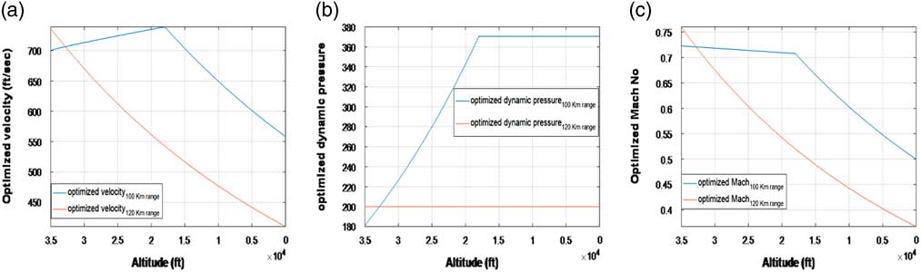
Generation of an optimal flight profile, in which parameters such as velocity, dynamic pressure, and Mach number are optimised, forms an essential part of the design of the GCM( Reference Jiang, Li, Li, Huang, Yang and Jiang 33 – Reference Jain and Tsiotras 36 ). This is important since the use of ad hoc profile or control policies to evaluate competing configurations may inappropriately penalise the performance of one configuration over another. Moreover, to avoid any undesirable aero-elastic phenomena, maximum dynamic pressure must be constrained. Thus, to guarantee optimised trajectory, it is important to optimise the aerodynamic flight profile and develop control policy for each configuration early in the design process. Two different types of optimised flight profiles (based on the dynamic pressure) are created to acquire ranges between 100 and 120 km, once SAK is air launched from an altitude of 35,000 ft. Table 2 depicts the flight profile developed for acquiring 100 km range.
Table 2 SAK geometric and mass properties

Graphical illustration of the optimised flight profile (for both 100 km and 120 km ranges) is depicted in Fig. 2. The velocity, dynamic pressure and Mach number are optimised for the entire flight regime (ranging from 35,000 ft to the ground target).

Figure 2 Optimal trajectories: aerodynamic flight profile.
2.5 Formulation of optimal control problem
In this section, steady-state values for the state and control variables are determined at each point of a pre-specified trajectory by computing an equilibria point of the differential equations specified in Equations (1)–(4). The key idea includes linearising the non-linear system along the trajectory, then using the resulting time-varying linearisation to obtain a time-varying state feedback controller that locally stabilises the system along the trajectory. The optimisation techniques similar to Refs. 37–41 enhanced SAK range to about 100 km with high accuracy. The problem is configured as a constrained optimisation problem( Reference Maqsood and Hiong Go 42 ), with an objective to determine an open loop control that optimises the specified performance index, subject to certain constraints( Reference Maqsood and Hiong Go 42 ). For optimisation, Matlab® non-linear constrained optimisation technique, based on Sequential Quadratic Programming (SQP) and quasi-Newton methods, is utilised. Steady states for the optimised trajectory were obtained for a co-ordinated turn flight at different turn rates as shown in the following equation:
 $${\rm Turn}\,{\rm rate}\,({\rm \dot{\rpsi }}){\equals}[{\minus}10,{\minus}7,{\minus}5,{\minus}3,{\minus}2,1,0,1,2,3,4,5,10]^{T\circ} \,/\,{\rm s}.$$
In order to generate the optimised trajectories at the desired turn rates (as specified in Equation (14), the performance measure that is minimised is defined in the following equation:
 $$J_{{min}} {\equals}w_{1} \dot{V}_{T} {\plus}w_{2} \dot{\ralpha }{\plus}w_{3} \dot{\rbeta }{\plus}w_{4} \dot{p}{\plus}w_{5} \dot{q}{\plus}w_{6} \dot{r}$$
where
 $$w_{1} ...w_{6} {\equals}1$$
and
$$w_{1} ...w_{6} {\equals}1$$
and
 $${\dot{\ralpha }}$$
,
$${\dot{\ralpha }}$$
,
 $${\dot{\rbeta }}$$
,
$${\dot{\rbeta }}$$
,
 $$\dot{p}$$
,
$$\dot{p}$$
,
 $$\dot{q}$$
,
$$\dot{q}$$
,
 $$\dot{r}$$
are the rate derivatives of velocity, angle-of-attack, side slip angle and roll, pitch and yaw rates, respectively. This cost function is minimised by the optimisation algorithm at each equilibria point of the pre-specified trajectory governed by the differential equations specified in Equations (1)–(4).
$$\dot{r}$$
are the rate derivatives of velocity, angle-of-attack, side slip angle and roll, pitch and yaw rates, respectively. This cost function is minimised by the optimisation algorithm at each equilibria point of the pre-specified trajectory governed by the differential equations specified in Equations (1)–(4).
The state and control variables utilised during the optimisation process are defined in the following equations:
 $$\matrix{ {{\mib{x}} {\equals}} \hfill & {[V_{T} ,\ralpha ,\rbeta ,\rphi ,\rtheta ,\rpsi ,p,q,r,P_{n} ,P_{e} ,h]^{T} ,\quad {\bf x}\in{\Bbb R}^{{12}} } \hfill \cr {{\mib{u}} {\equals}} \hfill & {[LCF,RCF]^{T} ,\quad {\bf u}\in{\Bbb R}^{2} } \hfill \cr } $$
where left control fin (LCF) and right control fin (RCF) are the control variables.
Path constraints along with the bounds on the state and control variables are defined in the following equation:
 $$\matrix{ {0\leq h\leq 35000ft,{\minus}3^{\circ} \,\lt\,\ralpha \,\lt\,6^{\circ} ,{\minus}6^{\circ} \,\lt\,\rbeta \,\lt\,6^{\circ} } \cr {Mach\leq 0.75,100km\leq Range\leq 120km.} \cr } $$
Terminal constraints are defined in the following equations:
 $$\matrix{ {} \hfill & {P_{n} (te){\minus}P_{{n_{{(te)}} }} \leq \Delta P_{n} ,} \hfill \cr {} \hfill & {P_{e} (te){\minus}P_{{e_{{(te)}} }} \leq \Delta P_{e} ,} \hfill \cr {} \hfill & {h(te){\minus}h_{{te}} \leq \Delta h,} \hfill \cr {} \hfill & {} \hfill \cr } $$
where
 $$P_{n} (te),P_{e} (te),h(te)$$
are the SAK co-ordinates at the terminal point,
$$P_{n} (te),P_{e} (te),h(te)$$
are the SAK co-ordinates at the terminal point,
 $$P_{{n_{{(te)}} }} ,P_{{e_{{(te)}} }} ,h_{{te}} $$
are the target co-ordinates and
$$P_{{n_{{(te)}} }} ,P_{{e_{{(te)}} }} ,h_{{te}} $$
are the target co-ordinates and
 $$\Delta P_{n} ,\Delta P_{e} ,\Delta h$$
are the permissible tolerances.
$$\Delta P_{n} ,\Delta P_{e} ,\Delta h$$
are the permissible tolerances.
According to the model assumptions, the orientation of SAK at any point 'b' can be described in terms of earlier point 'a', by the following equation:
 $$\matrix{ {{\mib{x}} (t_{a} ){\equals}{\b{x}} (t_{a} ){\plus}{\int}_{t_{a} }^{t_{b} } {\b{\dot{x}}} (t)dt,} \hfill \cr {} \hfill \cr } $$
where
 $${\mib{x}} (t_{b} )$$
and
$${\mib{x}} (t_{b} )$$
and
 $${\mib{x}} (t_{a} )$$
represents the state variables at time t
b
and t
a
, respectively.
$${\mib{x}} (t_{a} )$$
represents the state variables at time t
b
and t
a
, respectively.
An LQR control-based optimisation framework was, therefore, formulated which utilises a set of dynamic constraints represented by Equations (1)–(4), path constraints shown in Equations (17) and terminal constraints of Equations (18), while minimising the performance measure represented by Equation (15). As a result of the optimisation process, steady-state values for the state and control variables along various optimal trajectories (governed by Equation (14)) were obtained. The optimisation process utilised the optimal flight profile parameters (velocity, dynamic pressure and Mach number) evaluated in Section. 2 2.4.
During optimisation process, certain states and variables were kept fixed along the trim points of the optimal ballistic trajectories while other states and control variables were kept free for optimisation (Equation (20)) within the permissible ranges:
 $$\matrix{ {{\rm Fixed\_states}} {{\equals}[V_{T} ,h,\dot{\rphi },{\rm \dot{\rtheta },\dot{\rpsi }}]} \hfill \cr {{\rm Free\_states\,\, \hbox {\&}\;Controls}} \hfill {{\equals}[{\rm \ralpha ,\rbeta ,\rgamma },\rphi ,{\rm \rtheta },p,q,r,LCF,RCF]} \hfill \cr {} \hfill & {} \hfill \cr } $$
The numeric values of the V
T
and h utilised along different trim points of the trajectory are specified in Table 2. Also numeric values of
 $$\dot{\rphi }{\equals}0,{\rm \dot{\rtheta }}{\equals}0\,\&\,{\rm \dot{\rpsi }}{\equals}0$$
are used during optimisation. The optimal trim state value for
$$\dot{\rphi }{\equals}0,{\rm \dot{\rtheta }}{\equals}0\,\&\,{\rm \dot{\rpsi }}{\equals}0$$
are used during optimisation. The optimal trim state value for
 $${\rm \rgamma },{\rm \ralpha },{\rm \rbeta },\rphi ,{\rm \rtheta },p,q,r,LCF,RCF$$
within the permissible ranges was numerically ascertained along different trim points by the optimisation algorithm.
$${\rm \rgamma },{\rm \ralpha },{\rm \rbeta },\rphi ,{\rm \rtheta },p,q,r,LCF,RCF$$
within the permissible ranges was numerically ascertained along different trim points by the optimisation algorithm.
As a result of the optimisation, optimal trim values of the state and control variables were ascertained along trim points for the entire flight envelope (35,000-ground level). This included determining optimal trajectories for different turn rates governed by Equation (14). The trim values of the state and control variables along different trim points for one such optimal trajectory
 $$({\rm \dot{\rpsi }}{\equals}0)$$
are depicted in Table.3.
$$({\rm \dot{\rpsi }}{\equals}0)$$
are depicted in Table.3.
Table 3 Optimal state and control variables along equilibria points of the optimal trajectory (
 $$\dot{\psi }{\equals}0$$
)
$$\dot{\psi }{\equals}0$$
)
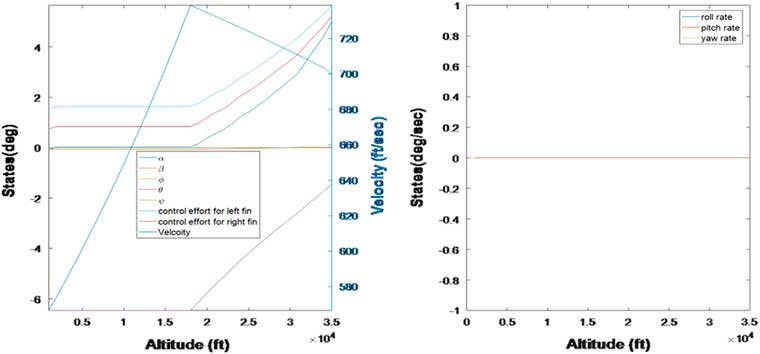
Figure 3 graphically depicts the values of steady-state control needed to guide the vehicle towards an intended target at 100 km range from the launching platform. System state response is also depicted in the same figure for the optimal
 $$\dot{\rpsi }{\equals}0$$
trajectory.
$$\dot{\rpsi }{\equals}0$$
trajectory.
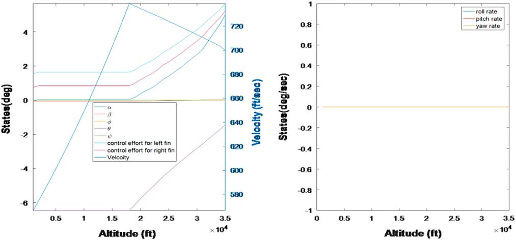
Figure 3 Optimal trajectories for the state and control variable for
 $$\dot{\psi }{\equals}0$$
trajectory.
$$\dot{\psi }{\equals}0$$
trajectory.
3.0 OPEN LOOP STABILITY AND CONTROLLABILITY ANALYSIS
3.1 Stability analysis
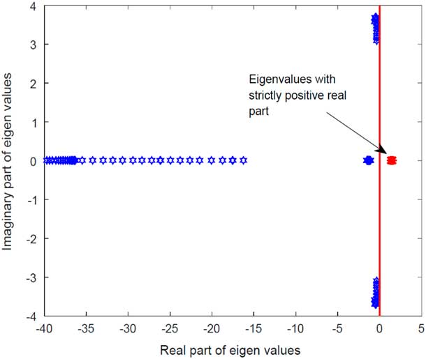
In this subsection, stability analysis of the SAK is performed utilising linear analysis tools. The stability aspects are determined for the system linearised about the equilibria point ascertained in Section 2.5. Eigen-value analysis revealed the system as unstable, as it contained a number of eigenvalues having strictly positive real part(s). The eigen-values are shown in Fig. 4.

Figure 4 Linearised system eigenvalues.
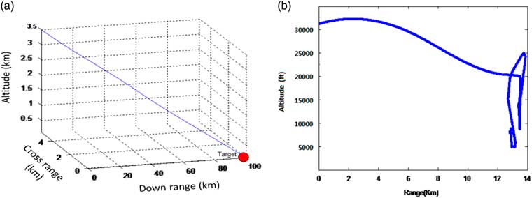
Due to this intrinsic instability, the non-linear system (governed by Equations (1)–(4)), when simulated for launch from an altitude of 35,000 ft, showed a complete unstable response (see Fig. 5). The SAK instead of following the optimised trajectory (Fig. 5(a)), exhibited an unstable response which resulted in the ballistic range of just 15 km (see Fig. 5(b)). This instability( Reference Christophersen, Pickell, Neidhoefer, Koller, Kannan and Johnson 43 ) caused the SAK to move in an uncontrolled manner immediately after launch. Resultantly, the SAK instead of following a gradual flight path angle showed a steep vertical descent.

Figure 5 Ballistic munition range.
3.2 Controllability analysis
Having shown in previous subsection that the system is intrinsically unstable, in this section, we determine the controllability aspects of the SAK. This is to ascertain that through suitable control, whether the unstable system can be made linearly/non-linearly controllable. The non-linear dynamic system governed by Equations (1)–(4) can be represented in the general form shown in the following:
 $${{\dot{\mib x}}} {\equals}{\bf F}(x(t),u(t))$$
A sufficient condition for the local controllability of the system (21) at
 $${\mib{x}} _{0} $$
is that the linearised system about
$${\mib{x}} _{0} $$
is that the linearised system about
 $${\mib{x}} _{0} $$
as defined in the following equation to be controllable:
$${\mib{x}} _{0} $$
as defined in the following equation to be controllable:
 $${\mib{\dot{x}}} {\equals}{\bf Ax}{\plus}{\bf Bu}.$$
By setting
 $${\mib{A}} {\equals}\left[ {{{\partial f({\mib{x}} ,{\mib{u}} )} \over {\partial {\mib{x}} }}} \right]_{{({\mib{x}} _{0} ,{\mib{u}} _{0} )}} $$
(
$${\mib{A}} {\equals}\left[ {{{\partial f({\mib{x}} ,{\mib{u}} )} \over {\partial {\mib{x}} }}} \right]_{{({\mib{x}} _{0} ,{\mib{u}} _{0} )}} $$
(
 $${\mib{A}} $$
 $$\in{\Bbb R}^{{n{\times}n}} $$
) and
$$\in{\Bbb R}^{{n{\times}n}} $$
) and
 $${\mib{B}} {\equals}\left[ {{{\partial {\mib{f}} ({\mib{x}} ,{\mib{u}} )} \over {\partial {\mib{u}} }}} \right]_{{({\mib{x}} _{0} ,{\mib{u}} _{0} )}} $$
(
$${\mib{B}} {\equals}\left[ {{{\partial {\mib{f}} ({\mib{x}} ,{\mib{u}} )} \over {\partial {\mib{u}} }}} \right]_{{({\mib{x}} _{0} ,{\mib{u}} _{0} )}} $$
(
 $${\mib{B}} $$
 $$\in{\Bbb R}^{{n{\times}m}} $$
), a controllability matrix
$$\in{\Bbb R}^{{n{\times}m}} $$
), a controllability matrix
 $${\mib{C}} $$
can be constructed as in Equation (23) to determine local controllability:
$${\mib{C}} $$
can be constructed as in Equation (23) to determine local controllability:
 $${\mib{C}} {\equals}\left[ {\matrix{ {{\mib{B}} ,{\mib{AB}} ,...,{\mib{A}} ^{n} {\mib{B}} } \cr } } \right],\quad {\mib{C}} \in{\Bbb R}^{{n{\times}nm}} .$$
A sufficient condition for the controllability of the linearised system is that the
 $${\Bbb R}^{{n{\times}nm}} $$
controllability matrix defined by Equation (23) has full row rank (i.e.
$${\Bbb R}^{{n{\times}nm}} $$
controllability matrix defined by Equation (23) has full row rank (i.e.
 $${\rm rank}(C){\equals}n$$
).
$${\rm rank}(C){\equals}n$$
).
In this study, the non-linear system, governed by Equations (1)–(4) was linearised about the equilibria (obtained in Section 2.5). To perform model linearisation, mathematical framework was developed in Matlab Simulink environment. In this model, the non-linear dynamics governed by Equations (1)–(4) along with all dependencies were incorporated. Resultantly, a linearised state space representation of the form specified in Equation (22) was ascertained about the equilibrium point.
The linearised system dynamics was concluded to be controllable as it had full rank Kalman matrix. This satisfied a sufficient condition for concluding the controllability of the original non-linear system, about the equilibria. This guaranteed that through a suitable control architecture, the unstable states of the system can be forced to follow the reference trajectory.
4.0 CONTROL LAW SYNTHESIS
The guidance schemes for the aerial munitions are in general based on either the classical approach using proportional navigation guidance (PNG) or on modern control theory (MCT). The proportional navigation used in the classical approach employs feedback with a constant gain from the angular rate of the line of sight between the target and the aerial vehicle, in order to minimise the final miss distance( Reference Kim, Kim and Park 22 , Reference Murtaugh and Criel 44 ). PNG has been most widely used in various guided weapons since the 1940s as it requires a small amount of information that can be easily obtained from seeker mounted on the weapons or the ground radar, such as the closing velocity and the line-of-sight (LOS) rate of guided weapons( Reference Zarchan 45 ). The modern control approach separates the guidance problem into estimation and optimum control. The former involves estimating the state variables, whereas in the latter, the optimum guidance law is derived in terms of time-varying feedback gains by a linear quadratic optimisation technique( Reference Lee, Jeon and Tahk 46 , Reference Stallard 47 ). To achieve optimality with guaranteed degree of robustness, the research work carried out in this study utilised a blend of both modern and classical approaches. LQR( Reference Hespanha 48 )-based control architecture is designed for stability purpose, where the Riccati equation is derived to provide time-varying feedback gains. Also PD-based navigation controller (utilising line of site principal) was utilised to ensure target tracking.
4.1 Stabilisation controller
In this section, control law synthesis(
Reference Dadkhah and Mettler
49
–
Reference Sujit, Saripalli and Sousa
52
) is performed for the SAK to meet the stabilisation issues after launch from the aerial platform (as discussed in Section 3.1). To achieve optimality with guaranteed degree of robustness, LQR(
Reference Hespanha
48
)-based control architecture is designed for stability purpose. The controller utilises the state information for providing the desired control. To simply the architecture, system non-effective states were excluded from the control loop. States mentioned in Equation (24) which includes (a) navigation state variables (x,y,h) and (b) heading state (
 $${\rm \rpsi }$$
) were neglected in the control design. This was because the system dynamics was independent of the variations in parameters of these states:
$${\rm \rpsi }$$
) were neglected in the control design. This was because the system dynamics was independent of the variations in parameters of these states:
 $$\matrix{ {{\mib{x}} _{{{\rm not\hbox{-}included}}} {\equals}[x,y,h,{\rm \rpsi }]^{T} .} \hfill \cr {} \hfill \cr } $$
The states utilised in the control architecture is represented in the following equation:
 $$\matrix{ {{\mib{x}} _{{{\rm utilized}}} {\equals}[V_{T} ,{\rm \ralpha ,\rbeta },\rphi ,{\rm \rtheta },p,q,r]^{T} .\quad {\mib{x}} _{{red}} \in{\Bbb {\rm R}}^{8} } \hfill \cr {} \hfill \cr } $$
The longitudinal dynamics of the reduced system is elaborated in the following equation:
 $$\matrix{ {{\mib{x}} _{{{\rm utilized}_{{{\rm (long)}}} }} {\equals}[V_{T} ,{\rm \ralpha },\rtheta ,q]^{T} ,\quad {\mib{x}} _{{{\rm red}_{{{\rm (long)}}} }} \in{\Bbb {\rm R}}^{4} } \hfill \cr {} \hfill \cr } $$
whereas the lateral dynamics are defined in the following equation:
 $$\matrix{ {{\mib{x}} _{{{\rm utilized}_{{{\rm (lat)}}} }} {\equals}[{\rm \rbeta },\rphi ,p,r]^{T} .\quad {\mib{x}} _{{{\rm red}_{{{\rm (lat)}}} }} \in{\Bbb {\rm R}}^{4} } \hfill \cr {} \hfill \cr } $$
The optimised values of the state (Q) and controller weighting matrices are shown below in the following equation:
 $$\matrix{ {} \hfill & {{\mib{Q}} {\equals}{\rm diag}[10,13,5,30,56,70,13,40]^{T} } \hfill \cr {} \hfill & {{\mib{R}} {\equals}{\rm diag}[10,4]^{T} } \hfill \cr } $$
Eigenvalue analysis of the linearised system with LQR controller was then performed to determine close loop stability. The system was identified to be stable as all the eigenvalues along the trim points of the optimised trajectory have strictly negative real parts. Eigenvalues analysis of the linearised system is depicted in Fig. 6.
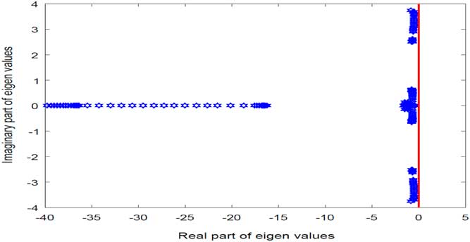
Figure 6 Eigenvalues of closed loop stable system.
In order to validate the viability and effectiveness of the proposed control architecture, a six DOF Simulink model incorporating vehicle, actuator and controller dynamics was developed in Matlab environment. Actuator dynamics was ascertained from the desired performance specification, as specified in Table 4. Stated parameters such as settling time, damping ratio and percentage overshoot, governs the dynamics of the actuator.
Table 4 Actuator performance parameters.
Based on these specifications, the second-order approximation of the actuator dynamics was made. This is elaborated in the following equation:
 $$\matrix{ {{\rm Actuator}\,{\rm dynamics}{\equals}G_{{DC}} \cdot {{w_{n}^{2} } \over {s^{2} {\plus}2{\rm \zeta }w_{n} s{\plus}w_{n}^{2} }},} \hfill \cr {} \hfill \cr } $$
where
 $$G_{{DC}} $$
is the DC gain ,
$$G_{{DC}} $$
is the DC gain ,
 $$w_{n} {\equals}\sqrt {{k \over m}} $$
is the natural frequency and
$$w_{n} {\equals}\sqrt {{k \over m}} $$
is the natural frequency and
 $${\rm \rzeta }$$
is the damping ratio.
$${\rm \rzeta }$$
is the damping ratio.
Simulation results (refer Fig. 7) showed a stable system response with the vehicle glide range extended to about 100 km. In comparison with the SAK open loop range of about 15 km, this was considerable improvement.
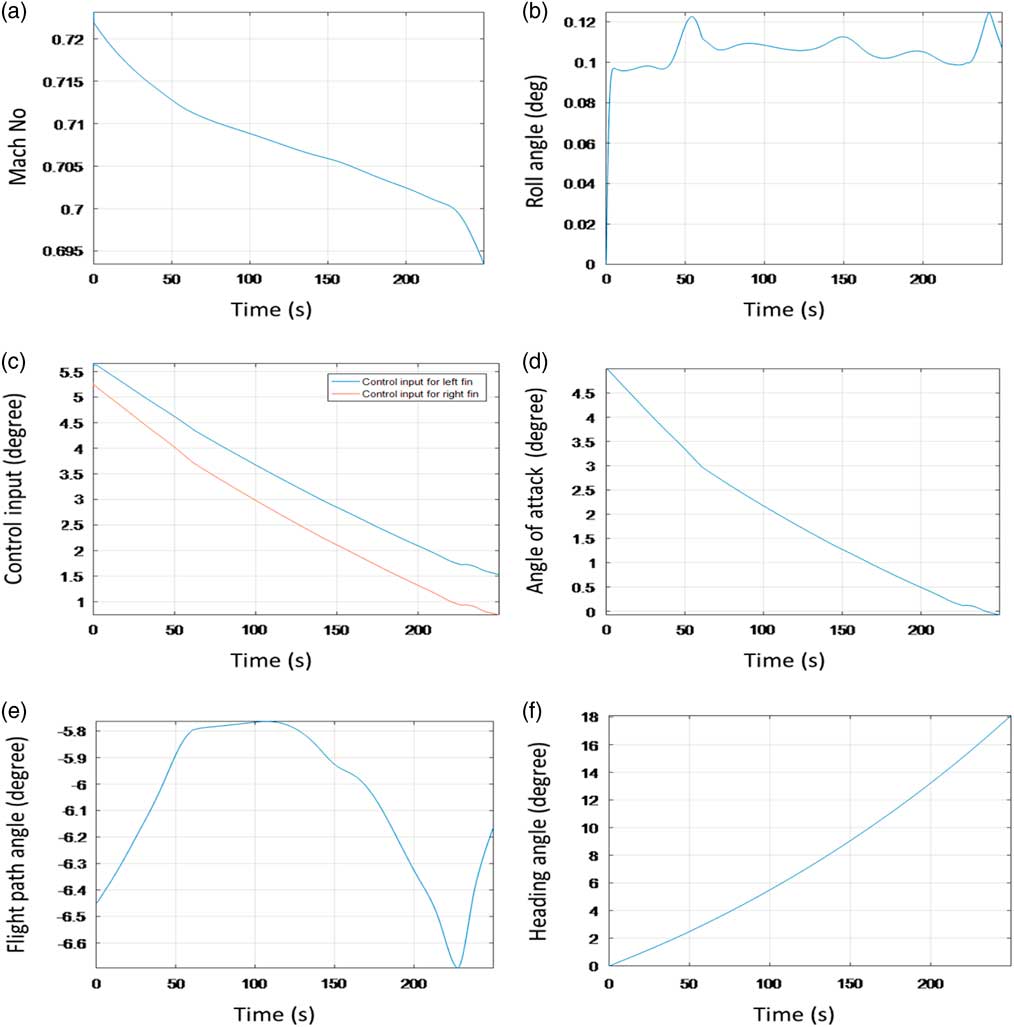
Figure 7 Close loop response with stabilisation control.
This considerable range enhancement was attained as the SAK followed the optimised trajectory under the control of the LQR based controller architecture. During simulation, system states exhibited a stable response. This concluded the effectiveness of the designed control architecture. However, it remains to highlight that actual implementation with navigation might result in range deterioration.
4.2 Tracking error
In the designed state feed-back LQR-based control architecture, problem of deviation from the desired course was encountered. In spite of having stable system response with theoretical range enhancement to about 100 km, the SAK has a considerable off shoot from the target location. This is shown in Fig. 8. The deviation from desired course was encountered as the designed control law did not utilise the directional information (
 $${\rm \rpsi })$$
provided by navigational equation (see Equation (4)). Both the longitudinal and lateral dynamics were independent from directional orientation provided by navigational equation (see Equation (4)). Accurate guidance to the target, therefore, requires incorporation of an additional control loop which minimises the drift in the heading.
$${\rm \rpsi })$$
provided by navigational equation (see Equation (4)). Both the longitudinal and lateral dynamics were independent from directional orientation provided by navigational equation (see Equation (4)). Accurate guidance to the target, therefore, requires incorporation of an additional control loop which minimises the drift in the heading.
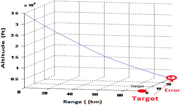
Figure 8 SAK response with stabilisation controller: range enhanced to 100 km but tracking problem encountered.
4.3 Implementation of tracking controller
Guidance is the very important component to accurately commanding a guided bomb to a target. In order to guide the SAK towards the target location, a tracking controller was added in the control architecture. Utilising the information of the present heading and the desired heading, estimates for the drift are made. Steering commands are then generated to precisely guide the SAK towards the target location. With the addition of the guidance controller( Reference Jamilnia and Naghash 53 – Reference Asadi, Sabzehparvar, Atkins and Talebi 55 ) in the GCM module, the framework for the control architecture was completed. Control law( Reference Fresconi, Cooper and Costello 56 ) based on PD controller for tracking is specified in the following equation:
 $$\matrix{ {{\rm Control}\,{\rm law}{\equals}A{\rm \rpsi }_{{{\rm error}}} {\plus}B{\rm \dot{\rpsi }}_{{{\rm error}}} } \hfill \cr {} \hfill \cr } $$
where
 $${\rm \rpsi }_{{{\rm error}}} $$
=
$${\rm \rpsi }_{{{\rm error}}} $$
=
 $${\rm \rpsi }_{{{\rm actual}}} $$
−
$${\rm \rpsi }_{{{\rm actual}}} $$
−
 $${\rm \rpsi }_{{{\rm error}}} $$
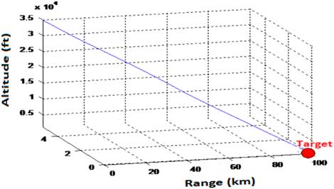
. Non-linear simulations carried out to evaluate the closed loop system response having both stability and guidance controllers exhibited a stable system response. Besides range enhanced to 100 km, the vehicle was accurately guided to the desired target location, with reduced CEP. This is shown in Fig. 9.
$${\rm \rpsi }_{{{\rm error}}} $$
. Non-linear simulations carried out to evaluate the closed loop system response having both stability and guidance controllers exhibited a stable system response. Besides range enhanced to 100 km, the vehicle was accurately guided to the desired target location, with reduced CEP. This is shown in Fig. 9.

Figure 9 SAK trajectory with stabilisation and guidance control.
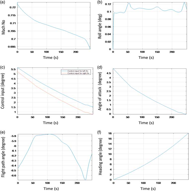
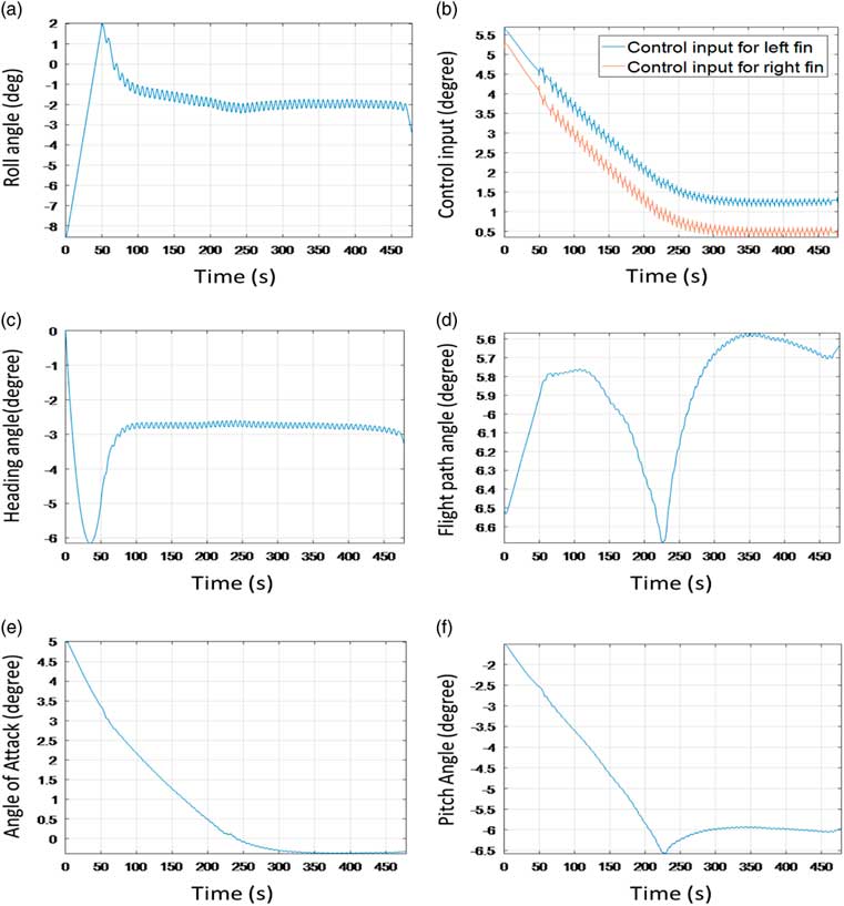
State and control variable response of the closed loop system is depicted in Fig. 10. It is clear from the figure that all the system states follow a trajectory to ensure that SAK after launch from the aircraft precisely hits the target within a range of about 100 km.
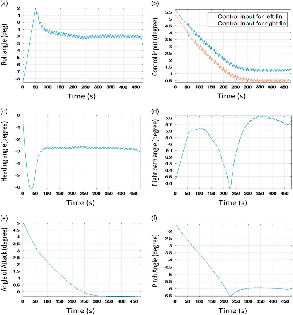
Figure 10 Close loop response with stabilisation and guidance controllers.
5.0 CONCLUSIONS
In this research, a framework is proposed for the design and development of a SAK that can modify the general purpose munition into a smart munition. Mathematical model for the development of integrated guidance and control module was presented. The starting point is a family of linear controllers with integral action designed for linearision of the non-linear equations of motion described in an appropriate state space. Based on this family, the method produces a gain scheduled controller that preserves the input–output properties of the original linear closed-loop systems as well as the closed-loop eigenvalues. The key feature of the method is the ability to automatically reconfigure the control inputs required to track the optimised trajectory, while maintaining the platform stability. The method is simple to apply and lead to an efficient architecture, which can convert the free fall munition into a smart munition. It enhanced the strike characteristics of the munition, their power and circular error probable (CEP) at cost levels which makes series production and mass scale utilisation economically acceptable.
The important results of this study are elaborated in Section 4 and are summarised below:
1. Development of SAK: An original SAK is developed which can carry the free fall munition to the desired target location.
2. Development of guidance and control module (GCM): This paper proposes an open framework for the design of guidance and control system for an original SAK, where both the guidance and control systems are designed simultaneously. The resulting trajectory tracking system achieves zero steady-state tracking error about the nominal trajectory. The guidance and control algorithm implemented could track the target using a single pair of control fins. This configuration although made the control architecture design more challenging but greatly reduced the modification cost.
3. Extended ballistic range and accuracy: Through the proposed design, the ballistic range of the munition has significantly been increased (about 100 km). This is comparable with what is achieved through majority of the existing modification kits, e.g., but not limited to Refs. 3 and 57. Apart from extended range, considerable improvement in accuracy is also achieved with improved CEP.
4. Open architecture and cost effective solution: The proposed framework provided an open solution which is cost effective, easy to implement and suitable for on-board implementation (see Section 2).
5. Limitations of the study: The investigations made in this research provides a mathematical-based analysis for designing a preliminary guidance and control system for the aerial munition. The theoretical validation of the proposed architecture was made through extensive simulations. The analysis provided is a first step towards full scale implementation of the SAK. So, the paper lays the ground for a research towards this direction, and justification to experiment/validate the methodology. The suggested model needs further hardware implementation and validation through flight demonstration utilising a realistic inertial/GNSS blended navigation system. This might lead to results which can vary the theoretically obtained ranges and CEP values. Therefore, the estimate of 100 km range and the CEP, once dovetailed with navigation module and practically implemented on hardware may expect some reduction.
6. Also the dearth in the literature made extremely difficult to compare our findings with other techniques. There have been numerous studies that implement similar technique on different problems. However, most of these studies (as mentioned in Section 1) provide very limited information about the details of the guidance and control architecture being employed for smart munitions. Keeping in view the peculiar advantages of different methodologies utilised in the literature, a well-established technique known to control community was implemented in this study. A blend of both modern and classical approaches was utilised to achieve optimal performance. The results achieved in this study are in line with Ref. 22, in which a similar guidance and control system algorithm for precision guided kits like JDAM is proposed.
7. Future outcomes: The modification kit proposed in this study can retrofit 500 lb MK-82 series free-fall munition into a smart munition. With requisite modifications, the proposed framework can be extended to retrofit other types of general purpose ballistic munitions as well.
APPENDIX A. SCHEMATICS DECRYPTION OF THE GUIDANCE AND CONTROL MODULE
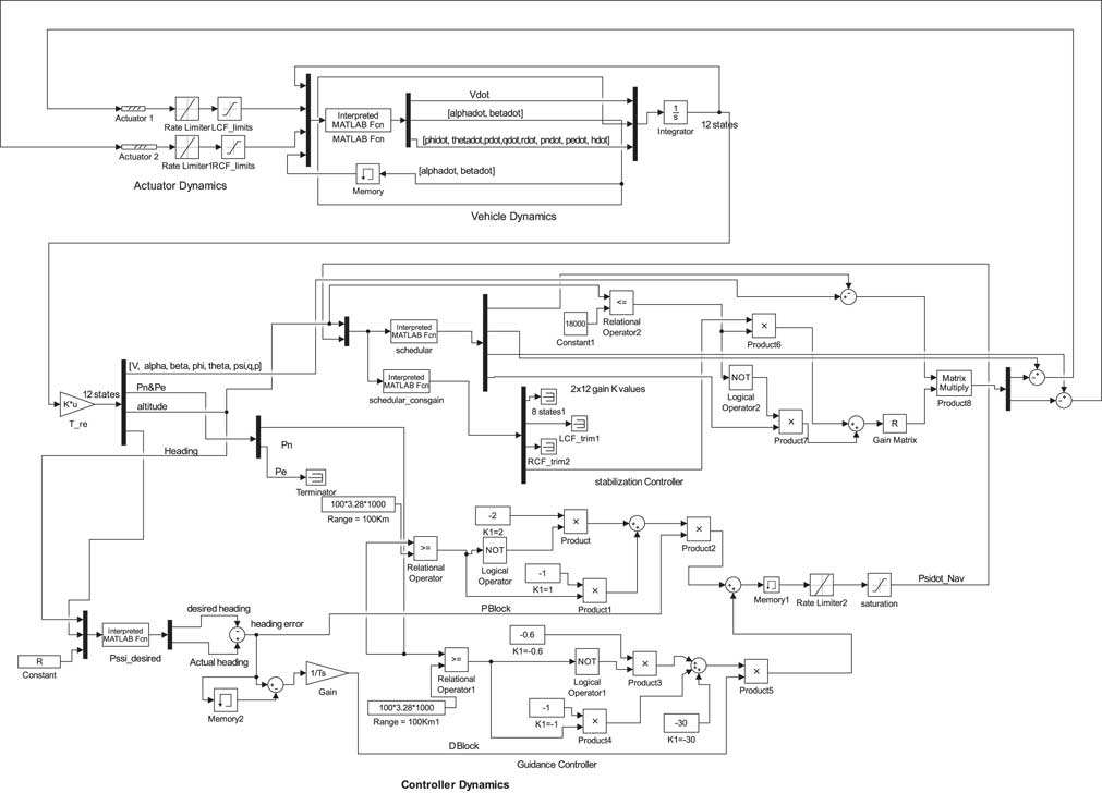
This appendix presents the schematic description of the GCM designed for the SAK. The detailed schematic layout is shown in Fig. 11. As shown in Fig. 11, the GCM mainly comprises of the three basic modules namely (a) actuator dynamics module, (b) vehicle dynamics module and (c) controller dynamics module. Individual details of these modules are explained in Fig. 11.

Figure 11 Schematic description of the GCM.
Vehicle dynamics module: The vehicle dynamics module is the main computational block of the architecture in which the non-linear 6-DOF equations of motion (refer Equations (1)–(4)) for the SAK are incorporated. The inputs to this module are the existing control information and state information at the previous step. Estimates for the updated estimates for the states are then made and are passed to the controller module.
Controller dynamics module: The controller dynamics module constitutes the control architecture and is composed of three main modules: (a) a scheduler, (b) a guidance controller and (c) a stabilisation controller. The updated state information from the vehicle dynamics module is provided to the guidance sub module. This information is utilised to estimate vehicle existing orientation in the 3D space. Based on the relative location of the vehicle w.r.t target, the estimates for drift in the existing heading are made. Steering commands are then generated to cancel this drift in the heading and guide the vehicle towards the target. The navigation controller is developed using classical PD control architecture. The drift information computed by guidance controller is also provided to the scheduler. The scheduler computes the desired values for the LQR controller gains and reference values for the equilibria state and control. This information is provided to the stabilisation controller. Utilising all available information, the LQR-based stabilisation controller finally generates desired controls for the actuator module.
Actuator dynamics module: The actuator dynamics module houses the actuator dynamics. The control commands are fed to the actuators module from the controller module. They are processed within the actuator module and then finally provided to the respective actuators of the two control fins.