


1 Introduction
Acoustic ducts of different shapes and sizes are ubiquitous in engineering applications as well as everyday life. From the curves and flare in a trombone (Hirschberg et al. Reference Hirschberg, Gilbert, Msallam and Wijnands1996; Rendón et al. Reference Rendón, Orduña-Bustamante, Narezo, Pérez-López and Sorrentini2010), or the call of an elephant propagating down its trunk (Gilbert et al. Reference Gilbert, Dalmont, Potier and Reby2014), to the design of automotive exhaust pipes and the curved air intakes on military aircraft (Brambley & Peake Reference Brambley and Peake2008), many ducts feature both a complex geometry and pressure waves of sufficient amplitude that nonlinearity should not be ignored. Until now, most work has dealt with either the geometrical problem of curved-duct acoustics in a linear regime or nonlinear acoustics in simple geometries. In this paper we shall address the combination of the two problems.
There are a number of works dealing with curved waveguides (see Rostafiński (Reference Rostafiński1991) for a fairly comprehensive review of early work). Current methods generally fall into one of three categories: perturbation methods (e.g. Ting & Miksis Reference Ting and Miksis1983) which limit the applicability of the solution to, for example, slender ducts; direct computation (e.g. Cabelli Reference Cabelli1980) limiting the physical insight; and methods based on the separation of variables. One such method, the multimodal method (MMM) – first proposed by Pagneux, Amir & Kergomard (Reference Pagneux, Amir and Kergomard1996) for the study of ducts of varying cross-section and subsequently generalised to two-dimensional (2-D) curved ducts (Félix & Pagneux Reference Félix and Pagneux2001), three-dimensional (3-D) curved ducts (Félix & Pagneux Reference Félix and Pagneux2002) and lined ducts (Bi et al. Reference Bi, Pagneux, Lafarge and Aurégan2006) – decomposes the pressure and velocity into a basis of straight-duct modes, relates these modes via an impedance matrix, and numerically solves the resulting equations throughout the duct, allowing for greater insight without the cost of restrictive approximations. This method shall form the basis of the present work, where we extend it to a weakly nonlinear regime. Similarly, ducts of varying width also have received much attention (see Campos (Reference Campos1984) for a review). Again, methods based on modal decomposition by Pagneux et al. (Reference Pagneux, Amir and Kergomard1996) shall influence our work.
The study of nonlinear acoustics in waveguides has hitherto largely focussed on the study of straight, uniform ducts or simplified wave approximations. Following the work of Hirschberg et al. (Reference Hirschberg, Gilbert, Msallam and Wijnands1996), who demonstrated that nonlinear effects give rise to wave steepening and shock formation in trombones, there has been much work on the modelling of acoustics in brass instruments (for example Thompson & Strong Reference Thompson and Strong2001; Gilbert, Menguy & Campbell Reference Gilbert, Menguy and Campbell2008; Rendón et al. Reference Rendón, Orduña-Bustamante, Narezo, Pérez-López and Sorrentini2010). Current literature in this area is typically restricted to one-dimensional (1-D) plane wave propagation, despite the fact that the plane wave approximation is a very poor approximation to the wave profile in a horn (Pagneux et al. Reference Pagneux, Amir and Kergomard1996). Other work dealing with non-planar wave propagation includes Fernando et al. (Reference Fernando, Druon, Coulouvrat and Marchiano2011), who use a multimodal method to calculate non-planar wave propagation in a straight duct. While this method has much in common with ours, it is not readily amenable to curved ducts due to the absence of a way of dealing with reflected waves.
The paper is set out in the following way. In § 2, we present an exposition of our method and derive its governing equations. This includes the introduction of our novel ‘nonlinear admittance’ term and the associated algebra governing it. In § 3 we derive the nonlinear boundary conditions for an infinite uniform outlet duct, including those which may be curved, and address the stability of such solutions. Our numerical method is presented in § 4, and in § 5 we show our numerical results, again, comparing with those previously published to illustrate the importance of taking nonlinear effects into account. In § 6 we investigate nonlinear propagation in ducts of identical length but differing geometry to show the effect different geometries have on the acoustic wave. In § 7 we introduce a new ‘nonlinear reflectance’ which takes into account the amplitude of the signal and use this to demonstrate how the reflectance of a duct changes with amplitude in previously published work.
2 Governing equations
Following the work of many classic texts (see for example Hamilton et al. (Reference Hamilton and Blackstock1998) chap. 3) we begin with the inviscid mass and momentum conservation equations
 $$\begin{eqnarray}\displaystyle & \displaystyle \frac{\unicode[STIX]{x2202}\unicode[STIX]{x1D70C}}{\unicode[STIX]{x2202}t}+\unicode[STIX]{x1D735}\boldsymbol{\cdot }(\unicode[STIX]{x1D70C}\boldsymbol{u})=0, & \displaystyle\end{eqnarray}$$
 $$\begin{eqnarray}\displaystyle & \displaystyle \unicode[STIX]{x1D70C}\left(\frac{\unicode[STIX]{x2202}\boldsymbol{u}}{\unicode[STIX]{x2202}t}+\boldsymbol{u}\boldsymbol{\cdot }\unicode[STIX]{x1D735}\boldsymbol{u}\right)=-\unicode[STIX]{x1D735}p, & \displaystyle\end{eqnarray}$$
 $\unicode[STIX]{x1D70C}$
,
$\unicode[STIX]{x1D70C}$
,
 $p$
and
$p$
and
 $\boldsymbol{u}$
are the fluid density, pressure, and velocity. We introduce non-dimensional variables of the form
$\boldsymbol{u}$
are the fluid density, pressure, and velocity. We introduce non-dimensional variables of the form  $$\begin{eqnarray}p=\unicode[STIX]{x1D70C}_{0}c_{0}^{2}\hat{p},\quad \unicode[STIX]{x1D70C}=\unicode[STIX]{x1D70C}_{0}\hat{\unicode[STIX]{x1D70C}},\quad \boldsymbol{u}=c_{0}\hat{\boldsymbol{u}},\end{eqnarray}$$
where
 $\unicode[STIX]{x1D70C}_{0}$
and
$\unicode[STIX]{x1D70C}_{0}$
and
 $c_{0}$
are the reference density and speed of sound for the stationary fluid respectively. Perturbations about a state of rest are then considered
$c_{0}$
are the reference density and speed of sound for the stationary fluid respectively. Perturbations about a state of rest are then considered
 $$\begin{eqnarray}\hat{p}=\hat{p}_{0}+\hat{p}^{\prime },\quad \hat{\unicode[STIX]{x1D70C}}=\hat{\unicode[STIX]{x1D70C}}_{0}+\hat{\unicode[STIX]{x1D70C}}^{\prime },\quad \hat{\boldsymbol{u}}=\hat{\boldsymbol{u}}^{\prime },\end{eqnarray}$$
with
 $\hat{p}^{\prime }\sim \hat{\unicode[STIX]{x1D70C}}^{\prime }\sim \hat{\boldsymbol{u}}^{\prime }\sim M$
where
$\hat{p}^{\prime }\sim \hat{\unicode[STIX]{x1D70C}}^{\prime }\sim \hat{\boldsymbol{u}}^{\prime }\sim M$
where
 $M<1$
is the perturbation Mach number, which is assumed to be small but finite. This approximation holds true in many situations. The conversion from Mach number to root mean square (r.m.s.) sound pressure level (SPL) in decibels for a sinusoidal pressure source in air at
$M<1$
is the perturbation Mach number, which is assumed to be small but finite. This approximation holds true in many situations. The conversion from Mach number to root mean square (r.m.s.) sound pressure level (SPL) in decibels for a sinusoidal pressure source in air at
 $20\,^{\circ }$
C is approximately
$20\,^{\circ }$
C is approximately
 $$\begin{eqnarray}\text{SPL}\sim (194+20\log _{10}M)~\text{dB}.\end{eqnarray}$$
For pressure sources such as that of the mouthpiece of the trombone when played fortissimo, SPLs can typically be around 170 dB corresponding to a Mach number of up to around 0.1. As such, the small but finite Mach number approximation is a very realistic one.
Discarding terms of
 $\mathit{O}(M^{3})$
and higher in (2.1a
) and (2.1b
) gives
$\mathit{O}(M^{3})$
and higher in (2.1a
) and (2.1b
) gives
 $$\begin{eqnarray}\displaystyle & \displaystyle \frac{1}{c_{0}}\frac{\unicode[STIX]{x2202}\hat{\unicode[STIX]{x1D70C}}^{\prime }}{\unicode[STIX]{x2202}t}+\unicode[STIX]{x1D735}\boldsymbol{\cdot }\hat{\boldsymbol{u}}^{\prime }=-\hat{\boldsymbol{u}}^{\prime }\boldsymbol{\cdot }\unicode[STIX]{x1D735}\hat{\unicode[STIX]{x1D70C}}^{\prime }-\hat{\unicode[STIX]{x1D70C}}^{\prime }\unicode[STIX]{x1D735}\boldsymbol{\cdot }\hat{\boldsymbol{u}}^{\prime }, & \displaystyle\end{eqnarray}$$
 $$\begin{eqnarray}\displaystyle & \displaystyle \frac{1}{c_{0}}\frac{\unicode[STIX]{x2202}\hat{\boldsymbol{u}}^{\prime }}{\unicode[STIX]{x2202}t}+\unicode[STIX]{x1D735}\hat{p}^{\prime }=-\hat{\boldsymbol{u}}^{\prime }\boldsymbol{\cdot }\unicode[STIX]{x1D735}\hat{\boldsymbol{u}}^{\prime }+\hat{\unicode[STIX]{x1D70C}}^{\prime }\unicode[STIX]{x1D735}\hat{p}^{\prime }, & \displaystyle\end{eqnarray}$$
 $\unicode[STIX]{x2202}\hat{\boldsymbol{u}}^{\prime }/\unicode[STIX]{x2202}t=-c_{0}\unicode[STIX]{x1D735}\hat{p}^{\prime }$
has been used in the quadratic term on the right-hand side of the momentum equation. In much of what will follow we will perform similar manipulations, substituting
$\unicode[STIX]{x2202}\hat{\boldsymbol{u}}^{\prime }/\unicode[STIX]{x2202}t=-c_{0}\unicode[STIX]{x1D735}\hat{p}^{\prime }$
has been used in the quadratic term on the right-hand side of the momentum equation. In much of what will follow we will perform similar manipulations, substituting
 $\mathit{O}(M)$
expressions for acoustical quantities into
$\mathit{O}(M)$
expressions for acoustical quantities into
 $\mathit{O}(M^{2})$
terms, noting that the error in doing so is
$\mathit{O}(M^{2})$
terms, noting that the error in doing so is
 $\mathit{O}(M^{3})$
which we are neglecting.
$\mathit{O}(M^{3})$
which we are neglecting.We now consider the entropy equation
 $$\begin{eqnarray}\frac{\text{D}S}{\text{D}t}=0,\end{eqnarray}$$
which holds everywhere, since our weakly nonlinear assumptions means any shocks are weak shocks. We shall take our fluid to have initially uniform entropy
 $S_{0}$
. By (2.6) our fluid will retain this value at all times. As a result, we may Taylor expand the equation of state
$S_{0}$
. By (2.6) our fluid will retain this value at all times. As a result, we may Taylor expand the equation of state
 $p=p(S,\unicode[STIX]{x1D70C})$
at fixed entropy about
$p=p(S,\unicode[STIX]{x1D70C})$
at fixed entropy about
 $\unicode[STIX]{x1D70C}=\unicode[STIX]{x1D70C}_{0}$
,
$\unicode[STIX]{x1D70C}=\unicode[STIX]{x1D70C}_{0}$
,
 $S=S_{0}$
, to get
$S=S_{0}$
, to get
 $$\begin{eqnarray}p^{\prime }=A\left(\frac{\unicode[STIX]{x1D70C}^{\prime }}{\unicode[STIX]{x1D70C}_{0}}\right)+\frac{B}{2!}\left(\frac{\unicode[STIX]{x1D70C}^{\prime }}{\unicode[STIX]{x1D70C}_{0}}\right)^{2}+\cdots =c_{0}^{2}\unicode[STIX]{x1D70C}^{\prime }+\frac{B}{2A}\frac{c_{0}^{2}}{\unicode[STIX]{x1D70C}_{0}}\unicode[STIX]{x1D70C}^{\prime 2}+\cdots \,,\end{eqnarray}$$
where
 $$\begin{eqnarray}A=\unicode[STIX]{x1D70C}_{0}\left(\frac{\unicode[STIX]{x2202}p}{\unicode[STIX]{x2202}\unicode[STIX]{x1D70C}}\right)_{S,0}=\unicode[STIX]{x1D70C}_{0}c_{0}^{2},\quad \text{and}\quad B=\unicode[STIX]{x1D70C}_{0}^{2}\left(\frac{\unicode[STIX]{x2202}^{2}p}{\unicode[STIX]{x2202}\unicode[STIX]{x1D70C}^{2}}\right)_{S,0}.\end{eqnarray}$$
For a perfect gas
 $B/A=\unicode[STIX]{x1D6FE}-1$
where
$B/A=\unicode[STIX]{x1D6FE}-1$
where
 $\unicode[STIX]{x1D6FE}$
is the ratio of specific heats. In non-dimensional variables
$\unicode[STIX]{x1D6FE}$
is the ratio of specific heats. In non-dimensional variables
 $$\begin{eqnarray}\hat{p}^{\prime }=\hat{\unicode[STIX]{x1D70C}}^{\prime }+\frac{B}{2A}\hat{\unicode[STIX]{x1D70C}}^{\prime 2}.\end{eqnarray}$$
Inverting this equation (correct to second order) gives
 $$\begin{eqnarray}\hat{\unicode[STIX]{x1D70C}}^{\prime }=\hat{p}^{\prime }-\frac{B}{2A}\hat{p}^{\prime 2},\end{eqnarray}$$
which can be used to eliminate density from the mass and momentum equations. This gives
 $$\begin{eqnarray}\displaystyle & \displaystyle \frac{1}{c_{0}}\frac{\unicode[STIX]{x2202}\hat{p}^{\prime }}{\unicode[STIX]{x2202}t}+\unicode[STIX]{x1D735}\boldsymbol{\cdot }\hat{\boldsymbol{u}}^{\prime }=-\hat{p}\unicode[STIX]{x1D735}\boldsymbol{\cdot }\hat{\boldsymbol{u}}^{\prime }-\hat{\boldsymbol{u}}^{\prime }\boldsymbol{\cdot }\unicode[STIX]{x1D735}\hat{p}+\frac{1}{c_{0}}\frac{B}{2A}\frac{\unicode[STIX]{x2202}}{\unicode[STIX]{x2202}t}(\hat{p}^{\prime 2}), & \displaystyle\end{eqnarray}$$
 $$\begin{eqnarray}\displaystyle & \displaystyle \frac{1}{c_{0}}\frac{\unicode[STIX]{x2202}\hat{\boldsymbol{u}}^{\prime }}{\unicode[STIX]{x2202}t}+\unicode[STIX]{x1D735}\hat{p}^{\prime }=-\hat{\boldsymbol{u}}^{\prime }\boldsymbol{\cdot }\unicode[STIX]{x1D735}\hat{\boldsymbol{u}}^{\prime }+\hat{p}^{\prime }\unicode[STIX]{x1D735}\hat{p}^{\prime }. & \displaystyle\end{eqnarray}$$
 $\unicode[STIX]{x1D714}$
,
$\unicode[STIX]{x1D714}$
,  $$\begin{eqnarray}\hat{p}=\mathop{\sum }_{a=-\infty }^{\infty }P^{a}(\boldsymbol{x})\text{e}^{-\text{i}a\unicode[STIX]{x1D714}t},\quad \hat{\boldsymbol{u}}=\mathop{\sum }_{a=-\infty }^{\infty }\boldsymbol{U}^{a}(\boldsymbol{x})\text{e}^{-\text{i}a\unicode[STIX]{x1D714}t},\end{eqnarray}$$
where
 $P^{-a}={P^{a}}^{\ast }$
and
$P^{-a}={P^{a}}^{\ast }$
and
 $\boldsymbol{U}^{-a}={\boldsymbol{U}^{a}}^{\ast }$
(with
$\boldsymbol{U}^{-a}={\boldsymbol{U}^{a}}^{\ast }$
(with
 $\ast$
denoting the complex conjugate) so that both
$\ast$
denoting the complex conjugate) so that both
 $\hat{p}$
and
$\hat{p}$
and
 $\hat{\boldsymbol{u}}$
are real (and can be substituted into quadratic terms without worry). Both
$\hat{\boldsymbol{u}}$
are real (and can be substituted into quadratic terms without worry). Both
 $P^{0}$
and
$P^{0}$
and
 $U^{0}$
are taken to be identically zero (see appendix A).
$U^{0}$
are taken to be identically zero (see appendix A).
Equations (2.11a ) and (2.11b ) then become
 $$\begin{eqnarray}\displaystyle \mathop{\sum }_{a=-\infty }^{\infty }(-\text{i}akP^{a}+\unicode[STIX]{x1D735}\boldsymbol{\cdot }\boldsymbol{U}^{a})\text{e}^{-\text{i}a\unicode[STIX]{x1D714}t} & = & \displaystyle \mathop{\sum }_{b,c=-\infty }^{\infty }\left(\vphantom{\frac{B}{2A}}-P^{b}\unicode[STIX]{x1D735}\boldsymbol{\cdot }\boldsymbol{U}^{c}-\boldsymbol{U}^{b}\boldsymbol{\cdot }\unicode[STIX]{x1D735}P^{c}\right.\nonumber\\ \displaystyle & & \displaystyle -\left.\frac{B}{2A}\text{i}(b+c)kP^{b}P^{c}\right)\text{e}^{-\text{i}(b+c)\unicode[STIX]{x1D714}t},\end{eqnarray}$$
 $$\begin{eqnarray}\displaystyle \mathop{\sum }_{a=-\infty }^{\infty }(-\text{i}ak\boldsymbol{U}^{a}+\unicode[STIX]{x1D735}P^{a})\text{e}^{-\text{i}a\unicode[STIX]{x1D714}t} & = & \displaystyle \mathop{\sum }_{b,c=-\infty }^{\infty }(-\boldsymbol{U}^{b}\boldsymbol{\cdot }\unicode[STIX]{x1D735}\boldsymbol{U}^{c}+P^{b}\unicode[STIX]{x1D735}P^{c})\text{e}^{-\text{i}(b+c)\unicode[STIX]{x1D714}t},\qquad\end{eqnarray}$$
 $k=\unicode[STIX]{x1D714}/c_{0}$
is the base wavenumber. Equating terms of the Fourier series yields
$k=\unicode[STIX]{x1D714}/c_{0}$
is the base wavenumber. Equating terms of the Fourier series yields  $$\begin{eqnarray}\displaystyle -\text{i}akP^{a}+\unicode[STIX]{x1D735}\boldsymbol{\cdot }\boldsymbol{U}^{a} & = & \displaystyle \mathop{\sum }_{b=-\infty }^{\infty }\left(-P^{a-b}\unicode[STIX]{x1D735}\boldsymbol{\cdot }\boldsymbol{U}^{b}-\boldsymbol{U}^{a-b}\boldsymbol{\cdot }\unicode[STIX]{x1D735}P^{b}-\frac{B}{2A}\text{i}akP^{b}P^{a-b}\right),\qquad\end{eqnarray}$$
 $$\begin{eqnarray}\displaystyle -\text{i}ak\boldsymbol{U}^{a}+\unicode[STIX]{x1D735}P^{a} & = & \displaystyle \mathop{\sum }_{b=-\infty }^{\infty }(-\boldsymbol{U}^{a-b}\boldsymbol{\cdot }\unicode[STIX]{x1D735}\boldsymbol{U}^{b}+P^{a-b}\unicode[STIX]{x1D735}P^{b}).\end{eqnarray}$$
2.1 Duct geometry

Figure 1. Illustration of the geometry of the duct.
Figure 1 illustrates the geometry of our duct. We define our duct by its centreline
 $\boldsymbol{q}(s)$
in terms of the longitudinal arc length
$\boldsymbol{q}(s)$
in terms of the longitudinal arc length
 $s$
from the pressure source inlet. The general position vector in the duct is given by
$s$
from the pressure source inlet. The general position vector in the duct is given by
 $$\begin{eqnarray}\boldsymbol{x}(s,r)=\boldsymbol{q}(s)+r\hat{\boldsymbol{n}},\end{eqnarray}$$
where
 $h_{-}(s)\leqslant r\leqslant h_{+}(s)$
(with
$h_{-}(s)\leqslant r\leqslant h_{+}(s)$
(with
 $h_{-}(s)<0$
) defines the transverse position inside the duct of width
$h_{-}(s)<0$
) defines the transverse position inside the duct of width
 $h=(h_{+}-h_{-})$
and
$h=(h_{+}-h_{-})$
and
 $\hat{\boldsymbol{n}}=\hat{\boldsymbol{n}}(s)$
is the unit normal to the duct defined by the Frenet–Serret formulas,
$\hat{\boldsymbol{n}}=\hat{\boldsymbol{n}}(s)$
is the unit normal to the duct defined by the Frenet–Serret formulas,
 $$\begin{eqnarray}\frac{\text{d}\boldsymbol{q}}{\text{d}s}=\hat{\boldsymbol{t}},\quad \frac{\text{d}\hat{\boldsymbol{t}}}{\text{d}s}=\unicode[STIX]{x1D705}(s)\hat{\boldsymbol{n}},\quad \frac{\text{d}\hat{\boldsymbol{n}}}{\text{d}s}=-\unicode[STIX]{x1D705}(s)\hat{\boldsymbol{t}},\end{eqnarray}$$
with
 $\unicode[STIX]{x1D705}(s)$
being the local curvature of the centreline and
$\unicode[STIX]{x1D705}(s)$
being the local curvature of the centreline and
 $\hat{\boldsymbol{t}}=\hat{\boldsymbol{t}}(s)$
the unit tangent vector to the centreline. The basis vectors and their corresponding Lamé coefficients are
$\hat{\boldsymbol{t}}=\hat{\boldsymbol{t}}(s)$
the unit tangent vector to the centreline. The basis vectors and their corresponding Lamé coefficients are
 $$\begin{eqnarray}\boldsymbol{e}_{s}=\hat{\boldsymbol{t}},\quad h_{s}=1-\unicode[STIX]{x1D705}r,\quad \boldsymbol{e}_{r}=\hat{\boldsymbol{n}},\quad h_{r}=1.\end{eqnarray}$$
Using these, equations (2.14a
) and (2.14b
) can now be expanded in their coordinate specific forms resulting in three coupled equations for the Fourier modes of pressure
 $P^{a}$
, longitudinal velocity
$P^{a}$
, longitudinal velocity
 $U^{a}$
and transverse velocity
$U^{a}$
and transverse velocity
 $V^{a}$
 $$\begin{eqnarray}\displaystyle & & \displaystyle -\text{i}akP^{a}+\frac{1}{1-\unicode[STIX]{x1D705}r}\frac{\unicode[STIX]{x2202}U^{a}}{\unicode[STIX]{x2202}s}+\frac{\unicode[STIX]{x2202}V^{a}}{\unicode[STIX]{x2202}r}-\frac{\unicode[STIX]{x1D705}V^{a}}{1-\unicode[STIX]{x1D705}r}\nonumber\\ \displaystyle & & \displaystyle \quad =\mathop{\sum }_{b=-\infty }^{\infty }\left(-\text{i}bkP^{a-b}P^{b}-\text{i}bkU^{a-b}U^{b}-\text{i}bkV^{a-b}V^{b}-\frac{B}{2A}\text{i}akP^{b}P^{a-b}\right),\end{eqnarray}$$
 $$\begin{eqnarray}\displaystyle & & \displaystyle -\text{i}akU^{a}+\frac{1}{1-\unicode[STIX]{x1D705}r}\frac{\unicode[STIX]{x2202}P^{a}}{\unicode[STIX]{x2202}s}\nonumber\\ \displaystyle & & \displaystyle \quad =\mathop{\sum }_{b=-\infty }^{\infty }\left(-\frac{U^{a-b}}{1-\unicode[STIX]{x1D705}r}\frac{\unicode[STIX]{x2202}U^{b}}{\unicode[STIX]{x2202}s}-V^{a-b}\frac{\unicode[STIX]{x2202}U^{b}}{\unicode[STIX]{x2202}r}+\frac{\unicode[STIX]{x1D705}}{1-\unicode[STIX]{x1D705}r}U^{a-b}V^{b}+\text{i}bkP^{a-b}U^{b}\right),\end{eqnarray}$$
 $$\begin{eqnarray}\displaystyle & & \displaystyle -\text{i}akV^{a}+\frac{\unicode[STIX]{x2202}P^{a}}{\unicode[STIX]{x2202}r}=\mathop{\sum }_{b=-\infty }^{\infty }\left(\frac{-U^{a-b}}{1-\unicode[STIX]{x1D705}r}\frac{\unicode[STIX]{x2202}V^{b}}{\unicode[STIX]{x2202}s}-V^{a-b}\frac{\unicode[STIX]{x2202}V^{b}}{\unicode[STIX]{x2202}r}-\frac{\unicode[STIX]{x1D705}}{1-\unicode[STIX]{x1D705}r}U^{a-b}U^{b}+\text{i}bkP^{a-b}V^{b}\right).\nonumber\\ \displaystyle & & \displaystyle\end{eqnarray}$$
From here, the temporal Fourier modes are expanded about a basis of spatial straight duct modes
 $$\begin{eqnarray}P^{a}=\mathop{\sum }_{p=0}^{\infty }P_{p}^{a}(s)\unicode[STIX]{x1D713}_{p}(s,r),\quad U^{a}=\mathop{\sum }_{p=0}^{\infty }U_{p}^{a}(s)\unicode[STIX]{x1D713}_{p}(s,r),\quad V^{a}=\mathop{\sum }_{p=0}^{\infty }V_{p}^{a}(s)\unicode[STIX]{x1D713}_{p}(s,r),\end{eqnarray}$$
where the
 $\unicode[STIX]{x1D713}_{p}$
satisfy
$\unicode[STIX]{x1D713}_{p}$
satisfy
 $$\begin{eqnarray}\frac{\text{d}^{2}\unicode[STIX]{x1D713}_{p}}{\text{d}r^{2}}+\unicode[STIX]{x1D702}_{p}^{2}\unicode[STIX]{x1D713}_{p}=0,\quad \int _{h_{-}}^{h_{+}}\unicode[STIX]{x1D713}_{p}\unicode[STIX]{x1D713}_{q}\,\text{d}r=\unicode[STIX]{x1D6FF}_{pq},\quad \left.\frac{\unicode[STIX]{x2202}\unicode[STIX]{x1D713}_{p}}{\unicode[STIX]{x2202}r}\right|_{r=h_{\pm }}=0,\end{eqnarray}$$
and are therefore given by
 $$\begin{eqnarray}\unicode[STIX]{x1D713}_{p}=C_{p}\cos \left(p\unicode[STIX]{x03C0}\frac{(r-h_{-})}{(h_{+}-h_{-})}\right),\quad C_{p}=\sqrt{\frac{2-\unicode[STIX]{x1D6FF}_{p0}}{h_{+}-h_{-}}},\quad \unicode[STIX]{x1D702}_{p}=\frac{p\unicode[STIX]{x03C0}}{h_{+}-h_{-}}.\end{eqnarray}$$
Here, we have expanded both the longitudinal and the transverse velocity components in terms of the duct basis, contrary to Félix & Pagneux (Reference Félix and Pagneux2001) who eliminated
 $V^{a}$
from the analogous linear equations at this point. It turns out that the higher radial derivatives that would arise from eliminating
$V^{a}$
from the analogous linear equations at this point. It turns out that the higher radial derivatives that would arise from eliminating
 $V^{a}$
from the above equations make it more complicated to apply the correct boundary conditions at the duct wall in the quadratic terms on the right-hand side, as described below. Projecting the equations onto the modal basis first, then eliminating the modal amplitudes of the transverse velocity
$V^{a}$
from the above equations make it more complicated to apply the correct boundary conditions at the duct wall in the quadratic terms on the right-hand side, as described below. Projecting the equations onto the modal basis first, then eliminating the modal amplitudes of the transverse velocity
 $V_{p}^{a}$
, turns out to be much simpler than eliminating the
$V_{p}^{a}$
, turns out to be much simpler than eliminating the
 $V^{a}$
from the above equations and then projecting onto the modal basis. At linear order, the two methods produce identical results (see appendix F).
$V^{a}$
from the above equations and then projecting onto the modal basis. At linear order, the two methods produce identical results (see appendix F).
As an aside, one may question the validity of expanding the temporal modes as a series of spatial duct modes, each with zero derivative on the boundary. This issue is dealt with in more detail in Pagneux et al. (Reference Pagneux, Amir and Kergomard1996), however we will briefly mention that this causes no difficulty, since an infinite series of terms with zero derivative at the boundary do not necessarily have a zero derivative. (For example, the function
 $y(x)=x$
has the Fourier cosine series expansion
$y(x)=x$
has the Fourier cosine series expansion
 $y(x)={\textstyle \frac{1}{2}}-(4/\unicode[STIX]{x03C0}^{2})\sum _{n=0}^{\infty }(1/(2n+1)^{2})\cos \big((2n+1)\unicode[STIX]{x03C0}x\big)$
, convergent for
$y(x)={\textstyle \frac{1}{2}}-(4/\unicode[STIX]{x03C0}^{2})\sum _{n=0}^{\infty }(1/(2n+1)^{2})\cos \big((2n+1)\unicode[STIX]{x03C0}x\big)$
, convergent for
 $x\in [0,1]$
. At both boundaries
$x\in [0,1]$
. At both boundaries
 $y(x)$
has derivative
$y(x)$
has derivative
 $1$
, despite each term in the sum having zero derivative at both boundaries.) Rather, care must be taken to apply the correct boundary conditions before expanding in terms of the
$1$
, despite each term in the sum having zero derivative at both boundaries.) Rather, care must be taken to apply the correct boundary conditions before expanding in terms of the
 $\unicode[STIX]{x1D713}_{p}$
basis.
$\unicode[STIX]{x1D713}_{p}$
basis.
We now wish to project the above equations onto the basis of modes. We first multiply the equations by a factor
 $(1-\unicode[STIX]{x1D705}r)$
, then by a general duct mode
$(1-\unicode[STIX]{x1D705}r)$
, then by a general duct mode
 $\unicode[STIX]{x1D713}_{p}$
and integrate across the duct width, ensuring to apply the no penetration boundary condition at the duct wall. This is given by
$\unicode[STIX]{x1D713}_{p}$
and integrate across the duct width, ensuring to apply the no penetration boundary condition at the duct wall. This is given by
 $$\begin{eqnarray}\boldsymbol{U}^{a}|_{r=h_{\pm }}\boldsymbol{\cdot }\boldsymbol{n}^{\pm }=0,\quad \boldsymbol{n}^{\pm }(s)=h_{\pm }^{\prime }\boldsymbol{e}_{s}-(1-\unicode[STIX]{x1D705}h_{\pm })\boldsymbol{e}_{r},\end{eqnarray}$$
where
 $\boldsymbol{n}^{\pm }$
are the normals to the duct wall. This corresponds to
$\boldsymbol{n}^{\pm }$
are the normals to the duct wall. This corresponds to
 $$\begin{eqnarray}h_{\pm }^{\prime }U^{a}=(1-\unicode[STIX]{x1D705}h_{\pm })V^{a}\quad \text{at }r=h_{\pm }.\end{eqnarray}$$
(Note that this simple relation between
 $U^{a}$
and
$U^{a}$
and
 $V^{a}$
at the duct wall would have been significantly complicated by nonlinear terms had we used (2.18c
) to eliminate
$V^{a}$
at the duct wall would have been significantly complicated by nonlinear terms had we used (2.18c
) to eliminate
 $V^{a}$
above.) Equation (2.23) can be used to eliminate
$V^{a}$
above.) Equation (2.23) can be used to eliminate
 $V^{a}$
at the boundaries. For example (summation convention assumed),
$V^{a}$
at the boundaries. For example (summation convention assumed),
 $$\begin{eqnarray}\int _{h_{-}}^{h_{+}}\frac{\unicode[STIX]{x2202}V^{a}}{\unicode[STIX]{x2202}r}\unicode[STIX]{x1D713}_{p}\,\text{d}r=\left[\frac{h^{\prime }}{1-\unicode[STIX]{x1D705}h}\unicode[STIX]{x1D713}_{p}\unicode[STIX]{x1D713}_{q}\right]_{h_{-}}^{h_{+}}U_{q}^{a}-\int _{h_{-}}^{h_{+}}\frac{\unicode[STIX]{x2202}\unicode[STIX]{x1D713}_{p}}{\unicode[STIX]{x2202}r}\unicode[STIX]{x1D713}_{q}\,\text{d}rV_{q}^{a}.\end{eqnarray}$$
Similarly,
 $$\begin{eqnarray}\int _{h_{-}}^{h_{+}}\frac{\unicode[STIX]{x2202}U^{a}}{\unicode[STIX]{x2202}s}\unicode[STIX]{x1D713}_{p}\,\text{d}r=\frac{\unicode[STIX]{x2202}U_{p}^{a}}{\unicode[STIX]{x2202}s}-[h^{\prime }\unicode[STIX]{x1D713}_{p}\unicode[STIX]{x1D713}_{q}]_{h_{-}}^{h_{+}}U_{q}^{a}-\int _{h_{-}}^{h_{+}}\frac{\unicode[STIX]{x2202}\unicode[STIX]{x1D713}_{p}}{\unicode[STIX]{x2202}s}\unicode[STIX]{x1D713}_{q}\,\text{d}rU_{q}^{a}.\end{eqnarray}$$
Other terms of note include
 $$\begin{eqnarray}\displaystyle \int _{h_{-}}^{h_{+}}U^{a-b}\frac{\unicode[STIX]{x2202}U^{b}}{\unicode[STIX]{x2202}s}\unicode[STIX]{x1D713}_{p}\,\text{d}r & = & \displaystyle \frac{1}{2}\frac{\text{d}}{\text{d}s}\left(\int _{h_{-}}^{h_{+}}\unicode[STIX]{x1D713}_{p}\unicode[STIX]{x1D713}_{q}\unicode[STIX]{x1D713}_{r}\,\text{d}r\right)U_{q}^{a-b}U_{r}^{b}-\frac{1}{2}\left[h^{\prime }\unicode[STIX]{x1D713}_{p}\unicode[STIX]{x1D713}_{q}\unicode[STIX]{x1D713}_{r}\right]_{h_{-}}^{h_{+}}U_{q}^{a-b}U_{r}^{b}\nonumber\\ \displaystyle & & \displaystyle +\,\frac{1}{2}\int _{h_{-}}^{h_{+}}\unicode[STIX]{x1D713}_{p}\unicode[STIX]{x1D713}_{q}\unicode[STIX]{x1D713}_{r}\,\text{d}r\left(U_{r}^{b}\frac{\text{d}}{\text{d}s}U_{q}^{a-b}+U_{q}^{a-b}\frac{\text{d}}{\text{d}s}U_{r}^{b}\right)\nonumber\\ \displaystyle & & \displaystyle -\,\frac{1}{2}\int _{h_{-}}^{h_{+}}\frac{\unicode[STIX]{x2202}\unicode[STIX]{x1D713}_{p}}{\unicode[STIX]{x2202}s}\unicode[STIX]{x1D713}_{q}\unicode[STIX]{x1D713}_{r}\,\text{d}rU_{q}^{a-b}U_{r}^{b},\end{eqnarray}$$
where the sum over
 $b$
has been reordered, and
$b$
has been reordered, and
 $$\begin{eqnarray}\displaystyle & & \displaystyle \int _{h_{-}}^{h_{+}}(1-\unicode[STIX]{x1D705}r)V^{a-b}\frac{\unicode[STIX]{x2202}U^{b}}{\unicode[STIX]{x2202}r}\unicode[STIX]{x1D713}_{p}\,\text{d}r\nonumber\\ \displaystyle & & \displaystyle \quad =[h^{\prime }U^{a-b}U^{b}\unicode[STIX]{x1D713}_{p}]_{h_{-}}^{h_{+}}-\int _{h_{-}}^{h_{+}}(1-\unicode[STIX]{x1D705}r)V^{a-b}U^{b}\frac{\unicode[STIX]{x2202}\unicode[STIX]{x1D713}_{p}}{\unicode[STIX]{x2202}r}\,\text{d}r\nonumber\\ \displaystyle & & \displaystyle \qquad +\,\unicode[STIX]{x1D705}\int _{h_{-}}^{h_{+}}V^{a-b}U^{b}\unicode[STIX]{x1D713}_{p}\,\text{d}r-\int _{h_{-}}^{h_{+}}(1-\unicode[STIX]{x1D705}r)\frac{\unicode[STIX]{x2202}V^{a-b}}{\unicode[STIX]{x2202}r}U^{b}\unicode[STIX]{x1D713}_{p}\,\text{d}r\nonumber\\ \displaystyle & & \displaystyle \quad =[h^{\prime }U^{a-b}U^{b}\unicode[STIX]{x1D713}_{p}]_{h_{-}}^{h_{+}}-\int _{h_{-}}^{h_{+}}(1-\unicode[STIX]{x1D705}r)V^{a-b}U^{b}\frac{\unicode[STIX]{x2202}\unicode[STIX]{x1D713}_{p}}{\unicode[STIX]{x2202}r}\,\text{d}r\nonumber\\ \displaystyle & & \displaystyle \qquad -\,\int _{h_{-}}^{h_{+}}\text{i}(a-b)k(1-\unicode[STIX]{x1D705}r)P^{a-b}U^{b}\unicode[STIX]{x1D713}_{p}\,\text{d}r+\int _{h_{-}}^{h_{+}}\frac{\unicode[STIX]{x2202}U^{a-b}}{\unicode[STIX]{x2202}s}U^{b}\unicode[STIX]{x1D713}_{p}\,\text{d}r,\end{eqnarray}$$
where the linear part of (2.18a
) has been used to substitute for
 $\unicode[STIX]{x2202}V^{a-b}/\unicode[STIX]{x2202}r$
. Using these, equations (2.18a
) and (2.18b
) become
$\unicode[STIX]{x2202}V^{a-b}/\unicode[STIX]{x2202}r$
. Using these, equations (2.18a
) and (2.18b
) become
 $$\begin{eqnarray}\displaystyle & & \displaystyle \frac{\text{d}}{\text{d}s}U_{p}^{a}-\text{i}ak\unicode[STIX]{x1D733}_{pq}[1-\unicode[STIX]{x1D705}r]P_{q}^{a}-\unicode[STIX]{x1D733}_{\{p\}q}U_{q}^{a}-\unicode[STIX]{x1D733}_{[\,p]q}[1-\unicode[STIX]{x1D705}r]V_{q}^{a}\nonumber\\ \displaystyle & & \displaystyle \quad =-\left(\text{i}bk+\text{i}ak\frac{B}{2A}\right)\unicode[STIX]{x1D733}_{pqr}[1-\unicode[STIX]{x1D705}r]P_{q}^{a-b}P_{r}^{b}-\text{i}bk\unicode[STIX]{x1D733}_{pqr}[1-\unicode[STIX]{x1D705}r]U_{q}^{a-b}U_{r}^{b}\nonumber\\ \displaystyle & & \displaystyle \qquad -\,\text{i}bk\unicode[STIX]{x1D733}_{pqr}[1-\unicode[STIX]{x1D705}r]V_{q}^{a-b}V_{r}^{b},\end{eqnarray}$$
 $$\begin{eqnarray}\displaystyle & & \displaystyle \frac{\text{d}}{\text{d}s}P_{p}^{a}-\text{i}ak\unicode[STIX]{x1D733}_{pq}[1-\unicode[STIX]{x1D705}r]U_{q}^{a}-([h^{\prime }\unicode[STIX]{x1D713}_{p}\unicode[STIX]{x1D713}_{q}]_{h_{-}}^{h_{+}}+\unicode[STIX]{x1D733}_{\{p\}q})P_{q}^{a}\nonumber\\ \displaystyle & & \displaystyle \quad =\left(\unicode[STIX]{x1D733}_{\{p\}qr}-\frac{\text{d}}{\text{d}s}(\unicode[STIX]{x1D733}_{pqr})\right)U_{q}^{a-b}U_{r}^{b}+\text{i}ak\unicode[STIX]{x1D733}_{pqr}[1-\unicode[STIX]{x1D705}r]P_{q}^{a-b}U_{r}^{b}\nonumber\\ \displaystyle & & \displaystyle \qquad +\,(\unicode[STIX]{x1D705}\unicode[STIX]{x1D733}_{pqr}+\unicode[STIX]{x1D733}_{[\,p]qr}[1-\unicode[STIX]{x1D705}r])U_{q}^{a-b}V_{r}^{b}-\unicode[STIX]{x1D733}_{pqr}\left(U_{r}^{b}\frac{\text{d}}{\text{d}s}U_{q}^{a-b}+U_{q}^{a-b}\frac{\text{d}}{\text{d}s}U_{r}^{b}\right)\!.\qquad\end{eqnarray}$$
 $\unicode[STIX]{x1D733}$
as a shorthand to denote integrals over the modes. Square brackets around an index represent radial derivatives on that mode, and curly brackets represent longitudinal derivatives. The square brackets after the
$\unicode[STIX]{x1D733}$
as a shorthand to denote integrals over the modes. Square brackets around an index represent radial derivatives on that mode, and curly brackets represent longitudinal derivatives. The square brackets after the
 $\unicode[STIX]{x1D733}$
are the integral kernel (assumed to be 1 if no brackets are present). So for example
$\unicode[STIX]{x1D733}$
are the integral kernel (assumed to be 1 if no brackets are present). So for example  $$\begin{eqnarray}\left.\begin{array}{@{}c@{}}\unicode[STIX]{x1D733}_{[\,p]q}=\displaystyle \int _{h_{-}}^{h_{+}}{\displaystyle \frac{\unicode[STIX]{x2202}\unicode[STIX]{x1D713}_{p}}{\unicode[STIX]{x2202}r}}\unicode[STIX]{x1D713}_{q}\,\text{d}r=(\unicode[STIX]{x1D733}_{p[q]})^{\text{T}}\\ \unicode[STIX]{x1D733}_{\{p\}qr}[1-\unicode[STIX]{x1D705}r]=\displaystyle \int _{h_{-}}^{h_{+}}{\displaystyle \frac{\unicode[STIX]{x2202}\unicode[STIX]{x1D713}_{p}}{\unicode[STIX]{x2202}s}}\unicode[STIX]{x1D713}_{q}\unicode[STIX]{x1D713}_{r}(1-\unicode[STIX]{x1D705}r)\,\text{d}r.\end{array}\right\}\end{eqnarray}$$
We now turn our attention to (2.18c
). Using the linear relationship between
 $V$
and
$V$
and
 $P$
from the left-hand side of (2.18c
) and the symmetry of mixed partials, we can find the linear expression for
$P$
from the left-hand side of (2.18c
) and the symmetry of mixed partials, we can find the linear expression for
 $\unicode[STIX]{x2202}V/\unicode[STIX]{x2202}s$
,
$\unicode[STIX]{x2202}V/\unicode[STIX]{x2202}s$
,
 $$\begin{eqnarray}\frac{\unicode[STIX]{x2202}V^{a}}{\unicode[STIX]{x2202}s}=\frac{1}{\text{i}ak}\frac{\unicode[STIX]{x2202}^{2}P^{a}}{\unicode[STIX]{x2202}s\unicode[STIX]{x2202}r}=(1-\unicode[STIX]{x1D705}r)\frac{\unicode[STIX]{x2202}U^{a}}{\unicode[STIX]{x2202}r}-\unicode[STIX]{x1D705}U^{a}.\end{eqnarray}$$
We also require the linear expression for
 $V_{p}^{a}$
in terms of
$V_{p}^{a}$
in terms of
 $P_{p}^{a}$
, also from the left-hand side of (2.18c
),
$P_{p}^{a}$
, also from the left-hand side of (2.18c
),
 $$\begin{eqnarray}V_{p}^{a}=\frac{1}{\text{i}ak}[\unicode[STIX]{x1D713}_{p}\unicode[STIX]{x1D713}_{q}]_{h_{-}}^{h_{+}}P_{q}^{a}-\frac{1}{\text{i}ak}\unicode[STIX]{x1D733}_{[\,p]q}P_{q}^{a}=\frac{1}{\text{i}ak}\unicode[STIX]{x1D733}_{p[q]}P_{q}^{a}.\end{eqnarray}$$
Using these, we can eliminate
 $V^{a}$
from the right-hand side of the projection of (2.18c
),
$V^{a}$
from the right-hand side of the projection of (2.18c
),
 $$\begin{eqnarray}\displaystyle & & \displaystyle -\text{i}ak\unicode[STIX]{x1D733}_{pq}[1-\unicode[STIX]{x1D705}r]V_{q}^{a}+([\unicode[STIX]{x1D713}_{p}\unicode[STIX]{x1D713}_{q}(1-\unicode[STIX]{x1D705}r)]_{h_{-}}^{h_{+}}-\unicode[STIX]{x1D733}_{[\,p]q}[1-\unicode[STIX]{x1D705}r]+\unicode[STIX]{x1D705}\unicode[STIX]{x1D6FF}_{pq})P_{q}^{a}\nonumber\\ \displaystyle & & \displaystyle \quad =\frac{1}{2}\left(\vphantom{\frac{h^{\prime 2}}{1-\unicode[STIX]{x1D705}h}}-[\unicode[STIX]{x1D713}_{p}\unicode[STIX]{x1D713}_{q}\unicode[STIX]{x1D713}_{r}(1-\unicode[STIX]{x1D705}r)]_{h_{-}}^{h_{+}}+\unicode[STIX]{x1D733}_{[\,p]qr}[1-\unicode[STIX]{x1D705}r]\right.\nonumber\\ \displaystyle & & \displaystyle \qquad -\left.\unicode[STIX]{x1D705}\unicode[STIX]{x1D733}_{pqr}-\left[\frac{h^{\prime 2}}{1-\unicode[STIX]{x1D705}h}\unicode[STIX]{x1D713}_{p}\unicode[STIX]{x1D713}_{q}\unicode[STIX]{x1D713}_{r}\right]_{h_{-}}^{h_{+}}\right)U_{q}^{a-b}U_{r}^{b}\nonumber\\ \displaystyle & & \displaystyle \qquad -\,\frac{1}{2k^{2}(a-b)b}(\unicode[STIX]{x1D733}_{[\,p]qr}[1-\unicode[STIX]{x1D705}r]-\unicode[STIX]{x1D705}\unicode[STIX]{x1D733}_{pqr})([\unicode[STIX]{x1D713}_{q}\unicode[STIX]{x1D713}_{s}]_{h_{-}}^{h_{+}}-\unicode[STIX]{x1D733}_{[q]s})([\unicode[STIX]{x1D713}_{r}\unicode[STIX]{x1D713}_{t}]_{h_{-}}^{h_{+}}-\unicode[STIX]{x1D733}_{[r]t})P_{s}^{a-b}P_{t}^{b}\nonumber\\ \displaystyle & & \displaystyle \qquad +\,\unicode[STIX]{x1D733}_{pqr}[1-\unicode[STIX]{x1D705}r]([\unicode[STIX]{x1D713}_{r}\unicode[STIX]{x1D713}_{t}]_{h_{-}}^{h_{+}}-\unicode[STIX]{x1D733}_{[r]t})P_{q}^{a-b}P_{t}^{b}.\end{eqnarray}$$
Using (2.31) and (2.32) we can eliminate
 $V$
from (2.28a
) and (2.28b
) to get
$V$
from (2.28a
) and (2.28b
) to get
 $$\begin{eqnarray}\displaystyle & \displaystyle \boldsymbol{u}^{\prime }+\unicode[STIX]{x1D648}\boldsymbol{p}+\unicode[STIX]{x1D642}\boldsymbol{u}={\mathcal{A}}[\boldsymbol{u},\boldsymbol{u}]+{\mathcal{B}}[\,\boldsymbol{p},\boldsymbol{p}], & \displaystyle\end{eqnarray}$$
 $$\begin{eqnarray}\displaystyle & \displaystyle \boldsymbol{p}^{\prime }-\unicode[STIX]{x1D649}\boldsymbol{u}-\unicode[STIX]{x1D643}\boldsymbol{p}={\mathcal{C}}[\boldsymbol{u},\boldsymbol{p}]+{\mathcal{D}}[\boldsymbol{u},\boldsymbol{u}], & \displaystyle\end{eqnarray}$$
 $\text{d}/\text{d}s$
. Matrix multiplication is defined over spatial modes in the following manner
$\text{d}/\text{d}s$
. Matrix multiplication is defined over spatial modes in the following manner  $$\begin{eqnarray}(\unicode[STIX]{x1D648}\boldsymbol{p})_{p}^{a}=\mathop{\sum }_{q=0}^{\infty }\unicode[STIX]{x1D648}_{pq}^{a}P_{q}^{a}.\end{eqnarray}$$
Calligraphic letters denote rank-5 tensors, with square brackets denoting the following action
 $$\begin{eqnarray}({\mathcal{A}}[\boldsymbol{x},\boldsymbol{y}])_{p}^{a}=\mathop{\sum }_{b=-\infty }^{\infty }\mathop{\sum }_{q,r=0}^{\infty }{\mathcal{A}}_{pqr}^{ab}X_{q}^{a-b}Y_{r}^{b}.\end{eqnarray}$$
The matrices and tensors are given by
 $$\begin{eqnarray}\displaystyle \unicode[STIX]{x1D648}_{pq}^{a} & = & \displaystyle -\text{i}ak\unicode[STIX]{x1D733}_{pq}[1-\unicode[STIX]{x1D705}r]-\frac{1}{\text{i}ak}\unicode[STIX]{x1D733}_{[\,p]s}[1-\unicode[STIX]{x1D705}r]\unicode[STIX]{x1D733}_{s[q]},\end{eqnarray}$$
 $$\begin{eqnarray}\displaystyle \unicode[STIX]{x1D649}_{pq}^{a} & = & \displaystyle \text{i}ak\unicode[STIX]{x1D733}_{pq}[1-\unicode[STIX]{x1D705}r],\end{eqnarray}$$
 $$\begin{eqnarray}\displaystyle \unicode[STIX]{x1D642}_{pq}^{a} & = & \displaystyle -\unicode[STIX]{x1D733}_{\{p\}q},\end{eqnarray}$$
 $$\begin{eqnarray}\displaystyle \unicode[STIX]{x1D643}_{pq}^{a} & = & \displaystyle -\unicode[STIX]{x1D733}_{p\{q\}},\end{eqnarray}$$
 $$\begin{eqnarray}\displaystyle {\mathcal{A}}_{pqr}^{ab} & = & \displaystyle -\text{i}bk\unicode[STIX]{x1D733}_{pqr}[1-\unicode[STIX]{x1D705}r]\nonumber\\ \displaystyle & & \displaystyle -\,\frac{1}{2}\unicode[STIX]{x1D733}_{[\,p]s}[1-\unicode[STIX]{x1D705}r](\unicode[STIX]{x1D649}^{-1})_{st}^{a}\left(\vphantom{\left[\frac{h}{1}\right]_{h}^{h}}-[\unicode[STIX]{x1D713}_{t}\unicode[STIX]{x1D713}_{q}\unicode[STIX]{x1D713}_{r}(1-\unicode[STIX]{x1D705}r)]_{h_{-}}^{h_{+}}+\unicode[STIX]{x1D733}_{[t]qr}[1-\unicode[STIX]{x1D705}r]\right.\nonumber\\ \displaystyle & & \displaystyle -\,\left.\unicode[STIX]{x1D705}\unicode[STIX]{x1D733}_{tqr}-\left[\frac{h^{\prime 2}}{1-\unicode[STIX]{x1D705}h}\unicode[STIX]{x1D713}_{t}\unicode[STIX]{x1D713}_{q}\unicode[STIX]{x1D713}_{r}\right]_{h_{-}}^{h_{+}}\right),\end{eqnarray}$$
 $$\begin{eqnarray}\displaystyle {\mathcal{B}}_{pqr}^{ab} & = & \displaystyle -\left(\text{i}bk+\text{i}ak\frac{B}{2A}\right)\unicode[STIX]{x1D733}_{pqr}[1-\unicode[STIX]{x1D705}r]-\frac{1}{\text{i}(a-b)k}\underbrace{\unicode[STIX]{x1D733}_{pst}[1-\unicode[STIX]{x1D705}r]\unicode[STIX]{x1D733}_{s[q]}\unicode[STIX]{x1D733}_{t[r]}}_{\unicode[STIX]{x1D733}_{p[q][r]}[1-\unicode[STIX]{x1D705}r]}\nonumber\\ \displaystyle & & \displaystyle -\,\unicode[STIX]{x1D733}_{[\,p]s}[1-\unicode[STIX]{x1D705}r](\unicode[STIX]{x1D649}^{-1})_{st}^{a}\left(\frac{-1}{2k^{2}(a-b)b}(\unicode[STIX]{x1D733}_{[t]uv}[1-\unicode[STIX]{x1D705}r]-\unicode[STIX]{x1D705}\unicode[STIX]{x1D733}_{tuv})\unicode[STIX]{x1D733}_{u[q]}\unicode[STIX]{x1D733}_{v[r]}\right.\nonumber\\ \displaystyle & & \displaystyle +\left.\unicode[STIX]{x1D733}_{tqu}[1-\unicode[STIX]{x1D705}r]\unicode[STIX]{x1D733}_{u[r]}\vphantom{\frac{1}{k}}\right),\end{eqnarray}$$
 $$\begin{eqnarray}\displaystyle {\mathcal{C}}_{pqr}^{ab} & = & \displaystyle \text{i}ak\unicode[STIX]{x1D733}_{pqr}[1-\unicode[STIX]{x1D705}r]+\frac{1}{\text{i}bk}\underbrace{(\unicode[STIX]{x1D705}\unicode[STIX]{x1D733}_{pqs}+\unicode[STIX]{x1D733}_{[\,p]qs}[1-\unicode[STIX]{x1D705}r])\unicode[STIX]{x1D733}_{s[r]}}_{\unicode[STIX]{x1D705}\unicode[STIX]{x1D733}_{pq[r]}+\unicode[STIX]{x1D733}_{[\,p]q[r]}[1-\unicode[STIX]{x1D705}r]}+\,2\unicode[STIX]{x1D733}_{pqs}\unicode[STIX]{x1D648}_{sr}^{b},\end{eqnarray}$$
 $$\begin{eqnarray}\displaystyle {\mathcal{D}}_{pqr}^{ab} & = & \displaystyle \unicode[STIX]{x1D733}_{\{p\}qr}-\frac{\text{d}}{\text{d}s}(\unicode[STIX]{x1D733}_{pqr})+2\unicode[STIX]{x1D733}_{pqs}\unicode[STIX]{x1D642}_{sr}^{b}.\end{eqnarray}$$
The
 $\unicode[STIX]{x1D733}$
can also be calculated analytically (see appendix B). Here,
$\unicode[STIX]{x1D733}$
can also be calculated analytically (see appendix B). Here,
 $\unicode[STIX]{x1D648}$
,
$\unicode[STIX]{x1D648}$
,
 $\unicode[STIX]{x1D649}$
,
$\unicode[STIX]{x1D649}$
,
 ${\mathcal{A}}$
,
${\mathcal{A}}$
,
 ${\mathcal{B}}$
and
${\mathcal{B}}$
and
 ${\mathcal{C}}$
encode the curvature of the duct, while
${\mathcal{C}}$
encode the curvature of the duct, while
 $\unicode[STIX]{x1D642},\unicode[STIX]{x1D643}$
and
$\unicode[STIX]{x1D642},\unicode[STIX]{x1D643}$
and
 ${\mathcal{D}}$
arise from variation in the duct width, vanishing when it is uniform.
${\mathcal{D}}$
arise from variation in the duct width, vanishing when it is uniform.
Due to the presence of evanescent modes these equations are numerically unstable and cannot be integrated directly (Pagneux et al. Reference Pagneux, Amir and Kergomard1996). Following the work of Félix & Pagneux (Reference Félix and Pagneux2001), we define a relation between the pressure and velocity in terms of the admittance. When solving for pressure it is easier to work with the admittance rather than the impedance to avoid inverting large matrices in the work that will follow.
The following relationship is defined
 $$\begin{eqnarray}\boldsymbol{u}=\unicode[STIX]{x1D654}\boldsymbol{p}+{\mathcal{Y}}[\,\boldsymbol{p},\boldsymbol{p}],\end{eqnarray}$$
where
 $\unicode[STIX]{x1D654}=\unicode[STIX]{x1D654}(s)$
is the linear part of the admittance (
$\unicode[STIX]{x1D654}=\unicode[STIX]{x1D654}(s)$
is the linear part of the admittance (
 $\unicode[STIX]{x1D654}=\unicode[STIX]{x1D655}^{-1}$
where
$\unicode[STIX]{x1D654}=\unicode[STIX]{x1D655}^{-1}$
where
 $\unicode[STIX]{x1D655}$
is the impedance matrix of Félix & Pagneux (Reference Félix and Pagneux2001)) and
$\unicode[STIX]{x1D655}$
is the impedance matrix of Félix & Pagneux (Reference Félix and Pagneux2001)) and
 ${\mathcal{Y}}={\mathcal{Y}}(s)$
is the second-order nonlinear correction to the impedance, henceforth referred to as the ‘nonlinear admittance’ term. We differentiate (2.37) with respect to
${\mathcal{Y}}={\mathcal{Y}}(s)$
is the second-order nonlinear correction to the impedance, henceforth referred to as the ‘nonlinear admittance’ term. We differentiate (2.37) with respect to
 $s$
,
$s$
,
 $$\begin{eqnarray}\boldsymbol{u}^{\prime }=\unicode[STIX]{x1D654}^{\prime }\boldsymbol{p}+\unicode[STIX]{x1D654}\boldsymbol{p}^{\prime }+{\mathcal{Y}}^{\prime }[\,\boldsymbol{p},\boldsymbol{p}]+{\mathcal{Y}}[\,\boldsymbol{p}^{\prime },\boldsymbol{p}]+{\mathcal{Y}}[\,\boldsymbol{p},\boldsymbol{p}^{\prime }],\end{eqnarray}$$
substitute in (2.33a ) and (2.33b ),
 $$\begin{eqnarray}\displaystyle & & \displaystyle -\unicode[STIX]{x1D648}\boldsymbol{p}-\unicode[STIX]{x1D642}\boldsymbol{u}+{\mathcal{A}}[\boldsymbol{u},\boldsymbol{u}]+{\mathcal{B}}[\,\boldsymbol{p},\boldsymbol{p}]=\unicode[STIX]{x1D654}^{\prime }\boldsymbol{p}+\unicode[STIX]{x1D654}(\unicode[STIX]{x1D649}\boldsymbol{u}+\unicode[STIX]{x1D643}\boldsymbol{p}+{\mathcal{C}}[\boldsymbol{u},\boldsymbol{p}]+{\mathcal{D}}[\boldsymbol{u},\boldsymbol{u}])\nonumber\\ \displaystyle & & \displaystyle \quad +\,{\mathcal{Y}}^{\prime }[\,\boldsymbol{p},\boldsymbol{p}]+{\mathcal{Y}}[\unicode[STIX]{x1D649}\boldsymbol{u}+\unicode[STIX]{x1D643}\boldsymbol{p},\boldsymbol{p}]+{\mathcal{Y}}[\,\boldsymbol{p},\unicode[STIX]{x1D649}\boldsymbol{u}+\unicode[STIX]{x1D643}\boldsymbol{p}]\end{eqnarray}$$
and use (2.37) to express
 $\boldsymbol{u}$
in terms of
$\boldsymbol{u}$
in terms of
 $\boldsymbol{p}$
 $$\begin{eqnarray}\displaystyle & & \displaystyle -\unicode[STIX]{x1D648}\boldsymbol{p}-\unicode[STIX]{x1D642}\unicode[STIX]{x1D654}\boldsymbol{p}-\unicode[STIX]{x1D642}{\mathcal{Y}}[\,\boldsymbol{p},\boldsymbol{p}]+{\mathcal{A}}[\unicode[STIX]{x1D654}\boldsymbol{p},\unicode[STIX]{x1D654}\boldsymbol{p}]+{\mathcal{B}}[\,\boldsymbol{p},\boldsymbol{p}]=\unicode[STIX]{x1D654}^{\prime }\boldsymbol{p}+\unicode[STIX]{x1D654}(\!\unicode[STIX]{x1D649}\unicode[STIX]{x1D654}\boldsymbol{p}+\unicode[STIX]{x1D649}{\mathcal{Y}}[\,\boldsymbol{p},\boldsymbol{p}]\nonumber\\ \displaystyle & & \displaystyle \quad +\,\unicode[STIX]{x1D643}\boldsymbol{p}+{\mathcal{C}}[\unicode[STIX]{x1D654}\boldsymbol{p},\boldsymbol{p}]+{\mathcal{D}}[\unicode[STIX]{x1D654}\boldsymbol{p},\unicode[STIX]{x1D654}\boldsymbol{p}]\!)+{\mathcal{Y}}^{\prime }[\,\boldsymbol{p},\boldsymbol{p}]+{\mathcal{Y}}[\unicode[STIX]{x1D649}\unicode[STIX]{x1D654}\boldsymbol{p}+\unicode[STIX]{x1D643}\boldsymbol{p},\boldsymbol{p}]+{\mathcal{Y}}[\,\boldsymbol{p},\unicode[STIX]{x1D649}\unicode[STIX]{x1D654}\boldsymbol{p}+\unicode[STIX]{x1D643}\boldsymbol{p}].\nonumber\\ \displaystyle & & \displaystyle\end{eqnarray}$$
This equation has two distinct orders of magnitude: terms linear in
 $\boldsymbol{p}$
, and terms quadratic in
$\boldsymbol{p}$
, and terms quadratic in
 $\boldsymbol{p}$
. We can equate linear terms and the quadratic terms separately to get two distinct equations
$\boldsymbol{p}$
. We can equate linear terms and the quadratic terms separately to get two distinct equations
 $$\begin{eqnarray}\displaystyle & \unicode[STIX]{x1D654}^{\prime }\boldsymbol{p}+\unicode[STIX]{x1D654}\unicode[STIX]{x1D649}\unicode[STIX]{x1D654}\boldsymbol{p}+\unicode[STIX]{x1D648}\boldsymbol{p}+\unicode[STIX]{x1D654}\unicode[STIX]{x1D643}\boldsymbol{p}+\unicode[STIX]{x1D642}\unicode[STIX]{x1D654}\boldsymbol{p}=0, & \displaystyle\end{eqnarray}$$
 $$\begin{eqnarray}\displaystyle & {\mathcal{Y}}^{\prime }[\,\boldsymbol{p},\boldsymbol{p}]+{\mathcal{Y}}[\unicode[STIX]{x1D649}\unicode[STIX]{x1D654}\boldsymbol{p},\boldsymbol{p}]+{\mathcal{Y}}[\,\boldsymbol{p},\unicode[STIX]{x1D649}\unicode[STIX]{x1D654}\boldsymbol{p}]+\unicode[STIX]{x1D654}\unicode[STIX]{x1D649}{\mathcal{Y}}[\,\boldsymbol{p},\boldsymbol{p}]+\unicode[STIX]{x1D654}{\mathcal{C}}[\unicode[STIX]{x1D654}\boldsymbol{p},\boldsymbol{p}]-{\mathcal{A}}[\unicode[STIX]{x1D654}\boldsymbol{p},\unicode[STIX]{x1D654}\boldsymbol{p}] & \displaystyle \nonumber\\ \displaystyle & -\,{\mathcal{B}}[\,\boldsymbol{p},\boldsymbol{p}]+{\mathcal{Y}}[\unicode[STIX]{x1D643}\boldsymbol{p},\boldsymbol{p}]+{\mathcal{Y}}[\,\boldsymbol{p},\unicode[STIX]{x1D643}\boldsymbol{p}]+\unicode[STIX]{x1D642}{\mathcal{Y}}[\,\boldsymbol{p},\boldsymbol{p}]+\unicode[STIX]{x1D654}{\mathcal{D}}[\unicode[STIX]{x1D654}\boldsymbol{p},\unicode[STIX]{x1D654}\boldsymbol{p}]=0. & \displaystyle\end{eqnarray}$$
 $\boldsymbol{p}$
, provided the linear part of the admittance and the nonlinear part of the admittance satisfy
$\boldsymbol{p}$
, provided the linear part of the admittance and the nonlinear part of the admittance satisfy  $$\begin{eqnarray}\displaystyle & \unicode[STIX]{x1D654}^{\prime }+\unicode[STIX]{x1D654}\unicode[STIX]{x1D649}\unicode[STIX]{x1D654}+\unicode[STIX]{x1D648}+\unicode[STIX]{x1D654}\unicode[STIX]{x1D643}+\unicode[STIX]{x1D642}\unicode[STIX]{x1D654}=0 & \displaystyle\end{eqnarray}$$
 $$\begin{eqnarray}\displaystyle & {\mathcal{Y}}^{\prime }[\unicode[STIX]{x1D644},\unicode[STIX]{x1D644}]+{\mathcal{Y}}[\unicode[STIX]{x1D649}\unicode[STIX]{x1D654},\unicode[STIX]{x1D644}]+{\mathcal{Y}}[\unicode[STIX]{x1D644},\unicode[STIX]{x1D649}\unicode[STIX]{x1D654}]+\unicode[STIX]{x1D654}\unicode[STIX]{x1D649}{\mathcal{Y}}[\unicode[STIX]{x1D644},\unicode[STIX]{x1D644}]+\unicode[STIX]{x1D654}{\mathcal{C}}[\unicode[STIX]{x1D654},\unicode[STIX]{x1D644}]-{\mathcal{A}}[\unicode[STIX]{x1D654},\unicode[STIX]{x1D654}] & \displaystyle \nonumber\\ \displaystyle & -\,{\mathcal{B}}[\unicode[STIX]{x1D644},\unicode[STIX]{x1D644}]+{\mathcal{Y}}[\unicode[STIX]{x1D643},\unicode[STIX]{x1D644}]+{\mathcal{Y}}[\unicode[STIX]{x1D644},\unicode[STIX]{x1D643}]+\unicode[STIX]{x1D642}{\mathcal{Y}}[\unicode[STIX]{x1D644},\unicode[STIX]{x1D644}]+\unicode[STIX]{x1D654}{\mathcal{D}}[\unicode[STIX]{x1D654},\unicode[STIX]{x1D654}]=0, & \displaystyle\end{eqnarray}$$
 $\unicode[STIX]{x1D644}_{pq}^{a}=\unicode[STIX]{x1D6FF}_{pq}\forall a$
is the identity tensor. Here, the square bracket notation acting on matrices denotes
$\unicode[STIX]{x1D644}_{pq}^{a}=\unicode[STIX]{x1D6FF}_{pq}\forall a$
is the identity tensor. Here, the square bracket notation acting on matrices denotes  $$\begin{eqnarray}(\unicode[STIX]{x1D655}{\mathcal{A}}[\unicode[STIX]{x1D653},\unicode[STIX]{x1D654}])_{pqr}^{ab}=\mathop{\sum }_{s,t,u=0}^{\infty }\unicode[STIX]{x1D655}_{pu}^{a}{\mathcal{A}}_{ust}^{ab}\unicode[STIX]{x1D653}_{sq}^{a-b}\unicode[STIX]{x1D654}_{tr}^{b}.\end{eqnarray}$$
These equations are solved from the outlet of the duct – where an appropriate radiation condition boundary condition is imposed – to the inlet. Once both parts of the admittance are found throughout the duct, they can be used to express the velocity modes in terms of pressure modes in (2.33b ). The result is a numerically stable first order equation for the pressure which can be solved from the inlet to the outlet using suitable initial conditions at the inlet to describe the waveform (both temporally and spatially) there,
 $$\begin{eqnarray}\boldsymbol{p}^{\prime }=\unicode[STIX]{x1D649}\unicode[STIX]{x1D654}\boldsymbol{p}+\unicode[STIX]{x1D649}{\mathcal{Y}}[\,\boldsymbol{p},\boldsymbol{p}]+{\mathcal{C}}[\unicode[STIX]{x1D654}\boldsymbol{p},\boldsymbol{p}]+\unicode[STIX]{x1D643}\boldsymbol{p}+{\mathcal{D}}[\unicode[STIX]{x1D654}\boldsymbol{p},\unicode[STIX]{x1D654}\boldsymbol{p}].\end{eqnarray}$$
Due to the varying admittance this equation takes into account a superposition of forwards and backwards travelling modes, as determined by the radiation condition at the outlet and any reflections due to the varying duct geometry, as well as the nonlinear interactions between modes. As such, this method is suitable for ducts where reflected waves are important, such as those that are curved or have an open/closed exit. For details of how to decompose this wave into its forward and backward propagating modes using a linear and nonlinear reflection coefficient, see § 7.
To summarise the proposed method, for a given duct and a given frequency, equations (2.42a ) and (2.42b ) need to be solved from the duct outlet, where an appropriate radiation condition is imposed, to the duct inlet. These equations are independent of the actual forcing at the inlet, and characterise the linear and weakly nonlinear response of the duct at the given frequency. One result of this is the linear and nonlinear admittance at the duct inlet, given by (2.37), which describes the input admittance of the duct and generalises the usual linear admittance to include Mach number dependent effects. Given the pressure forcing at the inlet, equation (2.44) may be solved from the inlet to the outlet to give the pressure oscillation at all points in the duct. In general, solving (2.42a ) and (2.42b ) is performed numerically, although analytic progress may be made in certain simplifying cases. One such case is a 1-D straight duct, given in appendix C. Another such case is a uniform constant-curvature duct, the solution to which may be used as the downstream impedance boundary condition for more complicated ducts, which we consider next.
3 An infinite uniform duct
Consider an infinitely long uniform duct of constant curvature for which we have only outgoing propagating waves and decaying evanescent waves. In such a duct no point can be distinguished from another longitudinally, therefore we must have the admittance being a fixed point of the admittance equations. To find the fixed points, we begin by combining (2.33a ) and (2.33b ) (ignoring the quadratic terms for the moment), to form a second-order ordinary differential equation for the pressure modes
 $$\begin{eqnarray}\boldsymbol{p}^{\prime \prime }+\unicode[STIX]{x1D649}\unicode[STIX]{x1D648}\boldsymbol{p}=0.\end{eqnarray}$$
Here we are considering a uniform duct of constant curvature, so
 $\unicode[STIX]{x1D642},\unicode[STIX]{x1D643}$
and the derivatives of
$\unicode[STIX]{x1D642},\unicode[STIX]{x1D643}$
and the derivatives of
 $\unicode[STIX]{x1D648}$
and
$\unicode[STIX]{x1D648}$
and
 $\unicode[STIX]{x1D649}$
vanish. As previously noted, this equation is numerically unstable. We can however make progress analytically. The solution in terms of forward and backwards modes is given by
$\unicode[STIX]{x1D649}$
vanish. As previously noted, this equation is numerically unstable. We can however make progress analytically. The solution in terms of forward and backwards modes is given by
 $$\begin{eqnarray}\boldsymbol{p}=\boldsymbol{p}^{+}+\boldsymbol{p}^{-}=\mathop{\sum }_{i=1}^{\infty }(c_{i}^{+}\boldsymbol{v}_{i}\text{e}^{\text{i}\unicode[STIX]{x1D706}_{i}s}+c_{i}^{-}\boldsymbol{v}_{i}\text{e}^{-i\unicode[STIX]{x1D706}_{i}s}),\end{eqnarray}$$
where the
 $\boldsymbol{v}_{i}$
are the eigenvectors of
$\boldsymbol{v}_{i}$
are the eigenvectors of
 $\unicode[STIX]{x1D649}\unicode[STIX]{x1D648}$
with eigenvalues
$\unicode[STIX]{x1D649}\unicode[STIX]{x1D648}$
with eigenvalues
 $\unicode[STIX]{x1D706}_{i}^{2}$
, with arbitrary
$\unicode[STIX]{x1D706}_{i}^{2}$
, with arbitrary
 $c_{i}^{+}$
and
$c_{i}^{+}$
and
 $c_{i}^{-}$
. Here, we have split the solution into forward and backward waves. The roots of the
$c_{i}^{-}$
. Here, we have split the solution into forward and backward waves. The roots of the
 $\unicode[STIX]{x1D706}_{i}$
are chosen as follows
$\unicode[STIX]{x1D706}_{i}$
are chosen as follows
 $$\begin{eqnarray}\unicode[STIX]{x1D706}_{i}=\left\{\begin{array}{@{}ll@{}}(\unicode[STIX]{x1D706}_{i}^{2})^{1/2},\quad & \unicode[STIX]{x1D706}_{i}^{2}>0,\\ \text{i}(-\unicode[STIX]{x1D706}_{i}^{2})^{1/2},\quad & \unicode[STIX]{x1D706}_{i}^{2}<0,\end{array}\right.\end{eqnarray}$$
to ensure either propagating or decaying evanescent modes in the positive direction. Based on extensive numerical evaluations, we observe that all of the eigenvectors of
 $\unicode[STIX]{x1D649}\unicode[STIX]{x1D648}$
are real (even though
$\unicode[STIX]{x1D649}\unicode[STIX]{x1D648}$
are real (even though
 $\unicode[STIX]{x1D649}\unicode[STIX]{x1D648}$
it is not necessarily symmetric for
$\unicode[STIX]{x1D649}\unicode[STIX]{x1D648}$
it is not necessarily symmetric for
 $\unicode[STIX]{x1D705}\neq 0$
). We now introduce the characteristic forward and backwards admittance, linearly relating the forwards and backwards modes
$\unicode[STIX]{x1D705}\neq 0$
). We now introduce the characteristic forward and backwards admittance, linearly relating the forwards and backwards modes
 $$\begin{eqnarray}\boldsymbol{u}^{\pm }=\unicode[STIX]{x1D654}^{\pm }\boldsymbol{p}^{\pm }.\end{eqnarray}$$
Using this, together with the linear equation relating pressure and velocity
 $(\boldsymbol{p}^{\pm })^{\prime }=\unicode[STIX]{x1D649}\boldsymbol{u}^{\pm }$
, we obtain and expression for
$(\boldsymbol{p}^{\pm })^{\prime }=\unicode[STIX]{x1D649}\boldsymbol{u}^{\pm }$
, we obtain and expression for
 $\unicode[STIX]{x1D654}^{\pm }$
 $$\begin{eqnarray}\unicode[STIX]{x1D654}^{\pm }=\pm \unicode[STIX]{x1D649}^{-1}\unicode[STIX]{x1D651}\unicode[STIX]{x1D726}\unicode[STIX]{x1D651}^{-1}=\pm \text{i}\unicode[STIX]{x1D649}^{-1}\sqrt{\unicode[STIX]{x1D649}\unicode[STIX]{x1D648}},\end{eqnarray}$$
where
 $\unicode[STIX]{x1D651}=(\boldsymbol{v}_{1},\boldsymbol{v}_{2},\ldots )$
and
$\unicode[STIX]{x1D651}=(\boldsymbol{v}_{1},\boldsymbol{v}_{2},\ldots )$
and
 $\unicode[STIX]{x1D726}=\text{diag}(\text{i}\unicode[STIX]{x1D706}_{1},~\text{i}\unicode[STIX]{x1D706}_{2},\ldots )$
. These can be shown to be fixed points of the linear admittance equation by direct substitution into (2.42a
) (again, ignoring
$\unicode[STIX]{x1D726}=\text{diag}(\text{i}\unicode[STIX]{x1D706}_{1},~\text{i}\unicode[STIX]{x1D706}_{2},\ldots )$
. These can be shown to be fixed points of the linear admittance equation by direct substitution into (2.42a
) (again, ignoring
 $\unicode[STIX]{x1D642}$
and
$\unicode[STIX]{x1D642}$
and
 $\unicode[STIX]{x1D643}$
as the duct is assumed uniform)
$\unicode[STIX]{x1D643}$
as the duct is assumed uniform)
 $$\begin{eqnarray}{\unicode[STIX]{x1D654}^{\pm }}^{\prime }=\unicode[STIX]{x1D649}^{-1}\sqrt{\unicode[STIX]{x1D649}\unicode[STIX]{x1D648}}\unicode[STIX]{x1D7EC}^{-1}\sqrt{\unicode[STIX]{x1D649}\unicode[STIX]{x1D648}}-\unicode[STIX]{x1D648}=0.\end{eqnarray}$$
Therefore,
 $\unicode[STIX]{x1D654}=\unicode[STIX]{x1D654}^{+}$
is the admittance of a uniform, constant-curvature duct supporting only outgoing propagating waves and decaying evanescent waves.
$\unicode[STIX]{x1D654}=\unicode[STIX]{x1D654}^{+}$
is the admittance of a uniform, constant-curvature duct supporting only outgoing propagating waves and decaying evanescent waves.
Using these characteristic linear admittances, we now wish to find the fixed points of the nonlinear admittance in (2.42b
). In order to do so we first introduce a matrix
 $\unicode[STIX]{x1D652}$
with columns given by the eigenvectors of
$\unicode[STIX]{x1D652}$
with columns given by the eigenvectors of
 $\unicode[STIX]{x1D654}^{\pm }\unicode[STIX]{x1D649}$
with corresponding eigenvalue matrix
$\unicode[STIX]{x1D654}^{\pm }\unicode[STIX]{x1D649}$
with corresponding eigenvalue matrix
 $\pm \unicode[STIX]{x1D726}$
. Fixed points of the nonlinear admittance equation satisfy
$\pm \unicode[STIX]{x1D726}$
. Fixed points of the nonlinear admittance equation satisfy
 $$\begin{eqnarray}{\mathcal{Y}}^{\pm }[\unicode[STIX]{x1D649}\unicode[STIX]{x1D654}^{\pm },\unicode[STIX]{x1D644}]+{\mathcal{Y}}^{\pm }[\unicode[STIX]{x1D644},\unicode[STIX]{x1D649}\unicode[STIX]{x1D654}^{\pm }]+\unicode[STIX]{x1D654}^{\pm }\unicode[STIX]{x1D649}{\mathcal{Y}}^{\pm }[\unicode[STIX]{x1D644},\unicode[STIX]{x1D644}]+\unicode[STIX]{x1D654}^{\pm }{\mathcal{C}}[\unicode[STIX]{x1D654}^{\pm },\unicode[STIX]{x1D644}]-{\mathcal{A}}[\unicode[STIX]{x1D654}^{\pm },\unicode[STIX]{x1D654}^{\pm }]-{\mathcal{B}}[\unicode[STIX]{x1D644},\unicode[STIX]{x1D644}]=0.\end{eqnarray}$$
We apply
 $\unicode[STIX]{x1D652}^{-1}$
on the left of this equation and
$\unicode[STIX]{x1D652}^{-1}$
on the left of this equation and
 $\unicode[STIX]{x1D651}$
to the right on both terms in the square brackets
$\unicode[STIX]{x1D651}$
to the right on both terms in the square brackets
 $$\begin{eqnarray}\displaystyle & & \displaystyle \unicode[STIX]{x1D652}^{-1}{\mathcal{Y}}^{\pm }[\pm \unicode[STIX]{x1D651}\unicode[STIX]{x1D726},\unicode[STIX]{x1D651}]+\unicode[STIX]{x1D652}^{-1}{\mathcal{Y}}^{\pm }[\unicode[STIX]{x1D651},\pm \unicode[STIX]{x1D651}\unicode[STIX]{x1D726}]+\unicode[STIX]{x1D652}^{-1}\unicode[STIX]{x1D654}^{\pm }\unicode[STIX]{x1D649}{\mathcal{Y}}^{\pm }[\unicode[STIX]{x1D651},\unicode[STIX]{x1D651}]\nonumber\\ \displaystyle & & \displaystyle \quad +\,\unicode[STIX]{x1D652}^{-1}\unicode[STIX]{x1D654}^{\pm }{\mathcal{C}}[\unicode[STIX]{x1D654}^{\pm }\unicode[STIX]{x1D651},\unicode[STIX]{x1D651}]-\unicode[STIX]{x1D652}^{-1}{\mathcal{A}}[\unicode[STIX]{x1D654}^{\pm }\unicode[STIX]{x1D651},\unicode[STIX]{x1D654}^{\pm }\unicode[STIX]{x1D651}]-\unicode[STIX]{x1D652}^{-1}{\mathcal{B}}[\unicode[STIX]{x1D651},\unicode[STIX]{x1D651}]=0,\end{eqnarray}$$
where we recall that
 $\unicode[STIX]{x1D651}$
,
$\unicode[STIX]{x1D651}$
,
 $\unicode[STIX]{x1D652}$
and
$\unicode[STIX]{x1D652}$
and
 $\unicode[STIX]{x1D726}$
each have an upper index and the matrix square bracket algebra is defined by (2.43). Next, we transform
$\unicode[STIX]{x1D726}$
each have an upper index and the matrix square bracket algebra is defined by (2.43). Next, we transform
 ${\mathcal{Y}}^{\pm }$
in the following manner
${\mathcal{Y}}^{\pm }$
in the following manner
 $$\begin{eqnarray}{\mathcal{Y}}^{\pm }[\boldsymbol{x},\boldsymbol{y}]=\unicode[STIX]{x1D652}\tilde{{\mathcal{Y}}}^{\pm }[\unicode[STIX]{x1D651}^{-1}\boldsymbol{x},\unicode[STIX]{x1D651}^{-1}\boldsymbol{y}]\end{eqnarray}$$
to obtain
 $$\begin{eqnarray}\displaystyle & & \displaystyle \tilde{{\mathcal{Y}}}^{\pm }[\pm \unicode[STIX]{x1D726},\unicode[STIX]{x1D644}]+\tilde{{\mathcal{Y}}}^{\pm }[\unicode[STIX]{x1D644},\pm \unicode[STIX]{x1D726}]\pm \unicode[STIX]{x1D726}\tilde{{\mathcal{Y}}}^{\pm }[\unicode[STIX]{x1D644},\unicode[STIX]{x1D644}]\nonumber\\ \displaystyle & & \displaystyle \quad +\,\unicode[STIX]{x1D652}^{-1}\unicode[STIX]{x1D654}^{\pm }{\mathcal{C}}[\unicode[STIX]{x1D654}^{\pm }\unicode[STIX]{x1D651},\unicode[STIX]{x1D651}]-\unicode[STIX]{x1D652}^{-1}{\mathcal{A}}[\unicode[STIX]{x1D654}^{\pm }\unicode[STIX]{x1D651},\unicode[STIX]{x1D654}^{\pm }\unicode[STIX]{x1D651}]-\unicode[STIX]{x1D652}^{-1}{\mathcal{B}}[\unicode[STIX]{x1D651},\unicode[STIX]{x1D651}]=0.\end{eqnarray}$$
As we are acting
 $\tilde{{\mathcal{Y}}}$
on purely diagonal matrices, its components can easily be read off
$\tilde{{\mathcal{Y}}}$
on purely diagonal matrices, its components can easily be read off
 $$\begin{eqnarray}(\tilde{{\mathcal{Y}}}^{\pm })_{pqr}^{ab}=\frac{(\unicode[STIX]{x1D652}^{-1}{\mathcal{A}}[\unicode[STIX]{x1D654}^{\pm }\unicode[STIX]{x1D651},\unicode[STIX]{x1D654}^{\pm }\unicode[STIX]{x1D651}]+\unicode[STIX]{x1D652}^{-1}{\mathcal{B}}[\unicode[STIX]{x1D651},\unicode[STIX]{x1D651}]-\unicode[STIX]{x1D652}^{-1}\unicode[STIX]{x1D654}^{\pm }{\mathcal{C}}[\unicode[STIX]{x1D654}^{\pm }\unicode[STIX]{x1D651},\unicode[STIX]{x1D651}])_{pqr}^{ab}}{\pm i\unicode[STIX]{x1D706}_{p}^{a}\pm i\unicode[STIX]{x1D706}_{q}^{a-b}\pm i\unicode[STIX]{x1D706}_{r}^{b}}.\end{eqnarray}$$
The reverse transformation is then applied to obtain the characteristic nonlinear part of the admittance. It can easily be seen that
 ${\mathcal{Y}}^{+}=-{\mathcal{Y}}^{-}$
. As the equation governing
${\mathcal{Y}}^{+}=-{\mathcal{Y}}^{-}$
. As the equation governing
 ${\mathcal{Y}}$
is linear, the
${\mathcal{Y}}$
is linear, the
 ${\mathcal{Y}}^{+}$
is unique (up to the equivalence class under summation – see appendix D) for a given choice of
${\mathcal{Y}}^{+}$
is unique (up to the equivalence class under summation – see appendix D) for a given choice of
 $\unicode[STIX]{x1D654}^{+}$
.
$\unicode[STIX]{x1D654}^{+}$
.
The linear and nonlinear impedances
 $\unicode[STIX]{x1D654}=\unicode[STIX]{x1D654}^{+}$
and
$\unicode[STIX]{x1D654}=\unicode[STIX]{x1D654}^{+}$
and
 ${\mathcal{Y}}={\mathcal{Y}}^{+}$
for a uniform constant-curvature duct may be used as a downstream boundary condition to (2.42a
) and (2.42b
) for arbitrary ducts. The solutions
${\mathcal{Y}}={\mathcal{Y}}^{+}$
for a uniform constant-curvature duct may be used as a downstream boundary condition to (2.42a
) and (2.42b
) for arbitrary ducts. The solutions
 $\unicode[STIX]{x1D654}=\unicode[STIX]{x1D654}^{+}$
and
$\unicode[STIX]{x1D654}=\unicode[STIX]{x1D654}^{+}$
and
 ${\mathcal{Y}}={\mathcal{Y}}^{+}$
correspond to the radiation condition
${\mathcal{Y}}={\mathcal{Y}}^{+}$
correspond to the radiation condition
 $$\begin{eqnarray}\boldsymbol{u}=\unicode[STIX]{x1D654}^{+}\boldsymbol{p}+{\mathcal{Y}}^{+}[\,\boldsymbol{p},\boldsymbol{p}],\end{eqnarray}$$
relating pressure and velocity modes at the exit, implying only outgoing waves and decaying evanescent waves in the uniform duct outlet of constant curvature.
3.1 Stability of fixed points of the admittance
One may question the stability of these fixed points by considering a small perturbation. For the linear part of the admittance take a small matrix perturbation
 $\unicode[STIX]{x1D73A}$
 $$\begin{eqnarray}\unicode[STIX]{x1D654}^{\pm }=\pm \unicode[STIX]{x1D649}^{-1}\unicode[STIX]{x1D651}\unicode[STIX]{x1D726}\unicode[STIX]{x1D651}^{-1}+\unicode[STIX]{x1D649}^{-1}\unicode[STIX]{x1D651}\unicode[STIX]{x1D73A}\unicode[STIX]{x1D651}^{-1}.\end{eqnarray}$$
In (2.42a ) this becomes
 $$\begin{eqnarray}\unicode[STIX]{x1D73A}^{\prime }=\mp \unicode[STIX]{x1D73A}\unicode[STIX]{x1D726}\mp \unicode[STIX]{x1D726}\unicode[STIX]{x1D73A}+\mathit{O}(\unicode[STIX]{x1D700}^{2}).\end{eqnarray}$$
Hence,
 $\unicode[STIX]{x1D654}^{+}$
is (at least Lyapunov) stable to small perturbations provided all the components of
$\unicode[STIX]{x1D654}^{+}$
is (at least Lyapunov) stable to small perturbations provided all the components of
 $\unicode[STIX]{x1D726}$
have
$\unicode[STIX]{x1D726}$
have
 $\text{Re}\unicode[STIX]{x1D726}\leqslant 0$
(remembering that we are solving in the negative
$\text{Re}\unicode[STIX]{x1D726}\leqslant 0$
(remembering that we are solving in the negative
 $s$
direction, so a positive exponential solution corresponds to a decaying perturbation) which is the case given our choice of decaying evanescent solutions. In a physical situation, we would in fact expect all of the components of
$s$
direction, so a positive exponential solution corresponds to a decaying perturbation) which is the case given our choice of decaying evanescent solutions. In a physical situation, we would in fact expect all of the components of
 $\unicode[STIX]{x1D6EC}$
to have at least a small negative real part (due to losses in the system), in which case this would be an asymptotically stable fixed point. On the other hand, due to the opposite signs our
$\unicode[STIX]{x1D6EC}$
to have at least a small negative real part (due to losses in the system), in which case this would be an asymptotically stable fixed point. On the other hand, due to the opposite signs our
 $\unicode[STIX]{x1D654}^{-}$
can be seen to be unstable (it is possible to form a stable
$\unicode[STIX]{x1D654}^{-}$
can be seen to be unstable (it is possible to form a stable
 $\unicode[STIX]{x1D654}^{-}$
corresponding to backwards propagating waves with forward decaying evanescent modes, however these would be unphysical). This justifies the use of
$\unicode[STIX]{x1D654}^{-}$
corresponding to backwards propagating waves with forward decaying evanescent modes, however these would be unphysical). This justifies the use of
 $\mathsf{Y}^{+}$
as a boundary condition for our linear admittance.
$\mathsf{Y}^{+}$
as a boundary condition for our linear admittance.
Similarly for the nonlinear part of the admittance consider a corresponding tensor perturbation
 $\unicode[STIX]{x1D700}$
 $$\begin{eqnarray}{\mathcal{Y}}={\mathcal{Y}}^{+}+\unicode[STIX]{x1D652}\unicode[STIX]{x1D700}[\unicode[STIX]{x1D651}^{-1},\unicode[STIX]{x1D651}^{-1}].\end{eqnarray}$$
In (2.42b ), we get
 $$\begin{eqnarray}\unicode[STIX]{x1D700}^{\prime }[\unicode[STIX]{x1D644},\unicode[STIX]{x1D644}]=-\unicode[STIX]{x1D700}[\unicode[STIX]{x1D726},\unicode[STIX]{x1D644}]-\unicode[STIX]{x1D700}[\unicode[STIX]{x1D644},\unicode[STIX]{x1D726}]-\unicode[STIX]{x1D726}\unicode[STIX]{x1D700}[\unicode[STIX]{x1D644},\unicode[STIX]{x1D644}].\end{eqnarray}$$
So similarly, we have (at least Lyapunov) stability provided all the components of
 $\unicode[STIX]{x1D726}$
have
$\unicode[STIX]{x1D726}$
have
 $\text{Re}\unicode[STIX]{x1D726}\leqslant 0$
, again justifying the use of
$\text{Re}\unicode[STIX]{x1D726}\leqslant 0$
, again justifying the use of
 ${\mathcal{Y}}^{+}$
as a boundary condition for the nonlinear admittance.
${\mathcal{Y}}^{+}$
as a boundary condition for the nonlinear admittance.
4 Numerical method
To implement our method we truncate the summations at
 $a_{max}$
temporal harmonics and
$a_{max}$
temporal harmonics and
 $p_{max}$
spatial modes. We shall not go into great detail on the convergence of this method with respect to the number of modes taken, but one can expect a Fourier series type convergence temporally. Spatially, the number of modes required varies greatly on the shape of the duct – uniform ducts typically require fewer modes than variable width ones to the correctly apply the boundary conditions. For an example of convergence, we consider the uniform curved duct described later in § 5.4 with sinusoidal planar source and
$p_{max}$
spatial modes. We shall not go into great detail on the convergence of this method with respect to the number of modes taken, but one can expect a Fourier series type convergence temporally. Spatially, the number of modes required varies greatly on the shape of the duct – uniform ducts typically require fewer modes than variable width ones to the correctly apply the boundary conditions. For an example of convergence, we consider the uniform curved duct described later in § 5.4 with sinusoidal planar source and
 $M=0.10$
. We define the error to be
$M=0.10$
. We define the error to be
 $$\begin{eqnarray}\text{error}={\displaystyle \frac{\displaystyle \int _{0}^{2\unicode[STIX]{x03C0}/\unicode[STIX]{x1D714}}\int _{0}^{s_{max}}\int _{h_{-}}^{h_{+}}|p-p_{ref}|\,\text{d}r\,\text{d}s\,\text{d}t}{\displaystyle \int _{0}^{2\unicode[STIX]{x03C0}/\unicode[STIX]{x1D714}}\int _{0}^{s_{max}}\int _{h_{-}}^{h_{+}}|p_{ref}|\,\text{d}r\,\text{d}s\,\text{d}t}}.\end{eqnarray}$$
We take our reference pressure
 $p_{ref}$
to be the solution produced by 10 spatial and 10 temporal modes. Figure 2 shows the error resulting from varying the number of spatial modes with fixed number of temporal and vice versa. Varying the number of spatial modes we obtain convergence
$p_{ref}$
to be the solution produced by 10 spatial and 10 temporal modes. Figure 2 shows the error resulting from varying the number of spatial modes with fixed number of temporal and vice versa. Varying the number of spatial modes we obtain convergence
 ${\sim}1/N^{3.21}$
. This is almost identical to the value obtained by Félix & Pagneux (Reference Félix and Pagneux2001). Varying the number of temporal modes we obtain convergence
${\sim}1/N^{3.21}$
. This is almost identical to the value obtained by Félix & Pagneux (Reference Félix and Pagneux2001). Varying the number of temporal modes we obtain convergence
 ${\sim}1/N^{1.28}$
. This number is dependant on the Mach number with smaller Mach numbers resulting in a greater convergence. For high Mach numbers the solution is described by a sawtooth wave throughout most of the duct (see appendix C) for which the convergence of the Fourier series is
${\sim}1/N^{1.28}$
. This number is dependant on the Mach number with smaller Mach numbers resulting in a greater convergence. For high Mach numbers the solution is described by a sawtooth wave throughout most of the duct (see appendix C) for which the convergence of the Fourier series is
 ${\sim}1/N$
. This gives the lower bound on the convergence.
${\sim}1/N$
. This gives the lower bound on the convergence.

Figure 2. Convergence of the method for (a) fixed number of temporal modes and (b) fixed number of spatial modes.
Convergence of the pressure solution can take quite a few modes (and consequently a large amount of computational time), depending on the frequency, Mach number and duct geometry, and in any given case a convergence study such as given in figure 2 would be needed to confirm convergence. However, good approximations can be made with very few modes – indeed many of the duct properties calculated later (such as power output and reflectance) can be calculated with good accuracy with as few as 5 spatial and 5 temporal modes for the parameters considered.
For the remainder of the paper we shall be dealing with ducts with an infinite uniform outlet. As such, we set
 $\unicode[STIX]{x1D654}=\unicode[STIX]{x1D654}^{+}$
for the initial condition of (2.42a
) and solve backwards through the duct to calculate
$\unicode[STIX]{x1D654}=\unicode[STIX]{x1D654}^{+}$
for the initial condition of (2.42a
) and solve backwards through the duct to calculate
 $\unicode[STIX]{x1D654}=\unicode[STIX]{x1D654}(s)$
at every point in the duct. Next, we solve (2.42b
) with initial condition
$\unicode[STIX]{x1D654}=\unicode[STIX]{x1D654}(s)$
at every point in the duct. Next, we solve (2.42b
) with initial condition
 ${\mathcal{Y}}={\mathcal{Y}}^{+}$
. Again, we solve backwards through the duct using the previously found values of
${\mathcal{Y}}={\mathcal{Y}}^{+}$
. Again, we solve backwards through the duct using the previously found values of
 $\unicode[STIX]{x1D654}$
in our evaluations of (2.42b
). Finally we solve (2.44) forwards through the duct using both the previously found
$\unicode[STIX]{x1D654}$
in our evaluations of (2.42b
). Finally we solve (2.44) forwards through the duct using both the previously found
 $\unicode[STIX]{x1D654}$
and
$\unicode[STIX]{x1D654}$
and
 ${\mathcal{Y}}$
in the evaluations of the equation. For the initial condition of the pressure we will generally be using a sinusoidal plane piston source so that
${\mathcal{Y}}$
in the evaluations of the equation. For the initial condition of the pressure we will generally be using a sinusoidal plane piston source so that
 $$\begin{eqnarray}P_{p}^{a}(0)={\textstyle \frac{1}{2}}\sqrt{h_{+}(0)-h_{-}(0)}M\unicode[STIX]{x1D6FF}_{p0}\unicode[STIX]{x1D6FF}^{|a|1}.\end{eqnarray}$$
Many other pressure sources can be modelled, with initial conditions chosen by decomposing the desired initial waveform into the modal/Fourier basis. Once both
 $\unicode[STIX]{x1D654}$
and
$\unicode[STIX]{x1D654}$
and
 ${\mathcal{Y}}$
are found throughout the duct for a particular wavenumber
${\mathcal{Y}}$
are found throughout the duct for a particular wavenumber
 $k$
, different pressure waveforms and amplitudes can be solved for without re-evaluation of (2.42a
) and (2.42b
).
$k$
, different pressure waveforms and amplitudes can be solved for without re-evaluation of (2.42a
) and (2.42b
).
To solve (2.42a
) and (2.42b
) we use a fixed step 4th order Runge–Kutta algorithm. For most cases this is adequate. Due to the temporally decoupled nature of these equations a high degree of parallelisation is possible. Indeed, when taking
 $a_{max}$
temporal modes there are
$a_{max}$
temporal modes there are
 $3a_{max}(a_{max}-1)/2$
independent equations for
$3a_{max}(a_{max}-1)/2$
independent equations for
 ${\mathcal{Y}}$
(for each
${\mathcal{Y}}$
(for each
 $a\in [1,a_{max}]$
we have
$a\in [1,a_{max}]$
we have
 $b\in [a-a_{max},a_{max}]$
minus the cases when
$b\in [a-a_{max},a_{max}]$
minus the cases when
 $b=0$
or
$b=0$
or
 $a=b$
) which can be solved in parallel. An issue, however, with this method is the large size of
$a=b$
) which can be solved in parallel. An issue, however, with this method is the large size of
 ${\mathcal{Y}}$
which scales like
${\mathcal{Y}}$
which scales like
 $\mathit{O}(a_{max}^{2}\,p_{max}^{3})$
with number of spatial modes
$\mathit{O}(a_{max}^{2}\,p_{max}^{3})$
with number of spatial modes
 $p_{max}$
. As a result, computational memory can be an issue. To overcome this, we opt to use a first-order exponential integrator method for the pressure as this requires the calculation and evaluation of
$p_{max}$
. As a result, computational memory can be an issue. To overcome this, we opt to use a first-order exponential integrator method for the pressure as this requires the calculation and evaluation of
 ${\mathcal{Y}}$
at fewer points.
${\mathcal{Y}}$
at fewer points.
If we consider the equation for the pressure as the sum of a linear operator
 $\unicode[STIX]{x1D647}$
acting on
$\unicode[STIX]{x1D647}$
acting on
 $\boldsymbol{p}$
and a nonlinear part
$\boldsymbol{p}$
and a nonlinear part
 ${\mathcal{N}}$
 $$\begin{eqnarray}\boldsymbol{p}^{\prime }=\unicode[STIX]{x1D647}\,\boldsymbol{p}+{\mathcal{N}}\end{eqnarray}$$
the exact solution is given by
 $$\begin{eqnarray}\boldsymbol{p}(s)=\exp \left(\int _{0}^{s}\unicode[STIX]{x1D647}(t)\,\text{d}t\right)\boldsymbol{p}(0)+\int _{0}^{s}\exp \left(\int _{t}^{s}\unicode[STIX]{x1D647}(u)\,\text{d}u\right){\mathcal{N}}(t)\,\text{d}t.\end{eqnarray}$$
We now consider a small step
 $\unicode[STIX]{x1D6FF}s$
and make the approximation that both
$\unicode[STIX]{x1D6FF}s$
and make the approximation that both
 $\unicode[STIX]{x1D647}$
and
$\unicode[STIX]{x1D647}$
and
 ${\mathcal{N}}$
are constant over this interval (in many cases this is valid – for infinite uniform ducts of constant curvature
${\mathcal{N}}$
are constant over this interval (in many cases this is valid – for infinite uniform ducts of constant curvature
 $\unicode[STIX]{x1D647}$
is a fixed point and so this method provides the correct solution to the linear problem), we obtain our stepping algorithm
$\unicode[STIX]{x1D647}$
is a fixed point and so this method provides the correct solution to the linear problem), we obtain our stepping algorithm
 $$\begin{eqnarray}\boldsymbol{p}(s+\unicode[STIX]{x1D6FF}s)=\exp (\unicode[STIX]{x1D6FF}s\unicode[STIX]{x1D647}(s))\boldsymbol{p}(s)-\unicode[STIX]{x1D647}^{-1}(\unicode[STIX]{x1D644}-\exp (\unicode[STIX]{x1D6FF}s\unicode[STIX]{x1D647}(s))){\mathcal{N}}(s).\end{eqnarray}$$
Matrix exponentiation was performed using a Fortran 90 routine written by John Burkardt based on the scaling and squaring algorithm used in MATLAB (see Moler & Van Loan Reference Moler and Van Loan2003). Other matrix operations were performed using LAPACK routines (Anderson et al.
Reference Anderson, Bai, Bischof, Blackford, Demmel, Dongarra, Du Croz, Greenbaum, Hammarling and McKenney1999). Running the code on an 8 core 3.40 GHz i7 processor with 15 GB of RAM can take of the order of tens of minutes when running with 5 spatial and 5 temporal modes, up to of the order of several hours when running with 10
 $+$
spatial and 10
$+$
spatial and 10
 $+$
temporal modes.
$+$
temporal modes.
4.1 Numerical viscosity
To overcome the errors (and numerical instabilities that can arise thereof) associated with truncation of the infinite series we add a numerical viscosity. If one considers (see (C 9) in appendix C, where we demonstrated the sawtooth wave as a solution to our equations), we can calculate the exact error associated with a finite truncation
 $$\begin{eqnarray}\text{error}=\frac{\text{i}\unicode[STIX]{x1D6FD}kM^{2}\sqrt{h_{+}-h_{-}}}{(1+\unicode[STIX]{x1D70E})^{2}}\text{e}^{\text{i}aks}\left(\mathop{\sum }_{b=a-a_{max}}^{a_{max}}\frac{a}{2(a-b)b(1+\unicode[STIX]{x1D70E})^{2}}-\mathop{\sum }_{b=-\infty }^{\infty }\frac{a}{2(a-b)b(1+\unicode[STIX]{x1D70E})^{2}}\right),\end{eqnarray}$$
where
 $\unicode[STIX]{x1D6FD}=1+B/2A$
and
$\unicode[STIX]{x1D6FD}=1+B/2A$
and
 $\unicode[STIX]{x1D70E}=s/(\unicode[STIX]{x1D6FD}Mk)$
is the distance normalised by the shock formation distance. After some algebra, this can be found to give
$\unicode[STIX]{x1D70E}=s/(\unicode[STIX]{x1D6FD}Mk)$
is the distance normalised by the shock formation distance. After some algebra, this can be found to give
 $$\begin{eqnarray}\text{error}=\frac{\text{i}\unicode[STIX]{x1D6FD}kM^{2}\sqrt{h_{+}-h_{-}}}{(1+\unicode[STIX]{x1D70E})^{2}}\text{e}^{\text{i}aks}\mathop{\sum }_{b=0}^{a}\frac{1}{a_{max}-b}.\end{eqnarray}$$
The summation can be approximated to
 $-\log (1-(a/a_{max}))$
using Euler’s asymptotic expansion of the harmonic numbers. The factor multiplying this is proportional to the pressure. This gives us a numerical viscosity term which can be deducted from the right-hand side of our pressure equation
$-\log (1-(a/a_{max}))$
using Euler’s asymptotic expansion of the harmonic numbers. The factor multiplying this is proportional to the pressure. This gives us a numerical viscosity term which can be deducted from the right-hand side of our pressure equation
 $$\begin{eqnarray}-\frac{\unicode[STIX]{x1D6FD}Mka}{1+\unicode[STIX]{x1D70E}}\log \left(1-\frac{a}{a_{max}}\right)P^{a}.\end{eqnarray}$$
For
 $a\ll a_{max}$
the logarithm can be Taylor expanded. For small distances we obtain the mode number squared numerical viscosity used by other authors (e.g. Fernando et al.
Reference Fernando, Druon, Coulouvrat and Marchiano2011)
$a\ll a_{max}$
the logarithm can be Taylor expanded. For small distances we obtain the mode number squared numerical viscosity used by other authors (e.g. Fernando et al.
Reference Fernando, Druon, Coulouvrat and Marchiano2011)
 $$\begin{eqnarray}\frac{\unicode[STIX]{x1D6FD}Mka^{2}}{a_{max}}P^{a},\end{eqnarray}$$
however, the logarithmic error is more accurate and provides better numerical results, and shall be used for the remainder of the paper. We incorporate the viscosity by modification of
 $\unicode[STIX]{x1D647}$
:
$\unicode[STIX]{x1D647}$
:
 $$\begin{eqnarray}\unicode[STIX]{x1D647}^{\unicode[STIX]{x1D656}}\mapsto \unicode[STIX]{x1D647}^{\unicode[STIX]{x1D656}}+\frac{\unicode[STIX]{x1D6FD}Mka}{1+\unicode[STIX]{x1D70E}}\log \left(1-\frac{a}{a_{max}}\right)\unicode[STIX]{x1D644}^{\unicode[STIX]{x1D656}}.\end{eqnarray}$$
As the sawtooth shape is the limiting form of all weakly nonlinear wave propagation (and the most harmonically rich) this provides a very good least upper bound for viscosity, preventing a ‘pooling’ of energy at truncation and ensuring that the simulations remain stable without compromising the solution unduly.
4.2 Ducts of increasing width
As observed by Pagneux et al. (Reference Pagneux, Amir and Kergomard1996), ducts increasing in width – particularly those with a large degree of flare – exhibit a strong degree of coupling between spatial modes. This coupling can prove problematic numerically, especially when a large number of spatial modes are retained. To ensure good accuracy in
 $\unicode[STIX]{x1D654}$
and especially in
$\unicode[STIX]{x1D654}$
and especially in
 ${\mathcal{Y}}$
, one must take smaller step sizes in the integration scheme as one increases
${\mathcal{Y}}$
, one must take smaller step sizes in the integration scheme as one increases
 $p_{max}$
. This further compounds the issue of computational complexity with increasing
$p_{max}$
. This further compounds the issue of computational complexity with increasing
 $p_{max}$
already noted.
$p_{max}$
already noted.
A workaround to this issue is to truncate the number of spatial modes in proportion to the change in duct width. We retain the number of modes
 $p_{ret}$
given by
$p_{ret}$
given by
 $$\begin{eqnarray}p_{ret}=\left\lceil p_{max}\frac{h_{+}(s)-h_{-}(s)}{h_{max}}\right\rceil .\end{eqnarray}$$
So, in an increasing width duct, as we solve backwards for
 $\unicode[STIX]{x1D654}$
and
$\unicode[STIX]{x1D654}$
and
 ${\mathcal{Y}}$
we truncate more modes as we approach the inlet. Then, solving forwards for the pressure, we start with a reduced number of modes and include more as we approach the exit. In practice, where solutions remain stable, with a sufficient maximum number of modes, this truncation makes little difference to the output – the transverse resolution is still preserved. This issue does not arise in ducts of decreasing width as modes undergo cutoff rather than cuton, however an unrelated mathematical difficulty does appear and is discussed in § 5.5.
${\mathcal{Y}}$
we truncate more modes as we approach the inlet. Then, solving forwards for the pressure, we start with a reduced number of modes and include more as we approach the exit. In practice, where solutions remain stable, with a sufficient maximum number of modes, this truncation makes little difference to the output – the transverse resolution is still preserved. This issue does not arise in ducts of decreasing width as modes undergo cutoff rather than cuton, however an unrelated mathematical difficulty does appear and is discussed in § 5.5.
5 Results
We now validate our method against previously published work and examine the effect of adding nonlinearity into problems where only linear acoustics was previously considered.
5.1 One-dimensional duct
In appendix C we show analytically that our method recovers both the Fubini (pre shock) and sawtooth (
 $\unicode[STIX]{x1D70E}>3$
) waves as solutions, where
$\unicode[STIX]{x1D70E}>3$
) waves as solutions, where
 $$\begin{eqnarray}\unicode[STIX]{x1D70E}=\frac{s}{\unicode[STIX]{x1D6FD}Mk}\end{eqnarray}$$
is the distance normalised to the shock formation distance (
 $\unicode[STIX]{x1D6FD}=1+(B/2A)$
). We now compare our numerical solution to the Blackstock solution – an asymptotic matching between the Fubini and sawtooth solutions (Blackstock Reference Blackstock1966). This has modal amplitudes given by
$\unicode[STIX]{x1D6FD}=1+(B/2A)$
). We now compare our numerical solution to the Blackstock solution – an asymptotic matching between the Fubini and sawtooth solutions (Blackstock Reference Blackstock1966). This has modal amplitudes given by
 $$\begin{eqnarray}B_{n}=\underbrace{\frac{2}{n\unicode[STIX]{x03C0}}P_{sh}}_{\mathit{Sawtooth}}+\underbrace{\frac{2}{n\unicode[STIX]{x03C0}\unicode[STIX]{x1D70E}}\int _{\unicode[STIX]{x1D6F7}_{sh}}^{\unicode[STIX]{x03C0}}\cos n(\unicode[STIX]{x1D6F7}-\unicode[STIX]{x1D70E}\sin \unicode[STIX]{x1D6F7})\,\text{d}\unicode[STIX]{x1D6F7}}_{\mathit{Fubini}}\end{eqnarray}$$
for
 $P_{sh}$
and
$P_{sh}$
and
 $\unicode[STIX]{x1D6F7}_{sh}$
satisfying
$\unicode[STIX]{x1D6F7}_{sh}$
satisfying
 $$\begin{eqnarray}P_{sh}=\sin (\unicode[STIX]{x1D70E}P_{sh}),\quad \unicode[STIX]{x1D6F7}_{sh}=\unicode[STIX]{x1D70E}\sin \unicode[STIX]{x1D6F7}_{sh}.\end{eqnarray}$$
Figure 3 shows the modal amplitudes plotted against distance through the duct normalised in terms of the shock formation distance, comparing our method with the Blackstock solution. Truncation was taken at 100 modes. Excellent agreement can be seen up to the 80th mode and as far as 10 times the shock formation distance. Even for modes above this the agreement is still very good – there is a slight underestimation at the point of shock formation with modal peaks occurring slightly further down the duct, however beyond that the error never exceeds 5 % even for the 100th mode.

Figure 3. Comparison of modal amplitudes along the waveguide between our method and the analytic Blackstock solution for (a) modes 1–5 and (b) modes 10–80.
5.2 Two-dimensional straight duct
The case of non-planar wave propagation in a 2-D waveguide was dealt with by Fernando et al. (Reference Fernando, Druon, Coulouvrat and Marchiano2011). In appendix D we give a partial proof of the equivalence of our method with theirs. Here, we consider a numerical example from that paper to demonstrate the equivalence of our methods. Figure 4 shows the result of sending a finite amplitude plane wave down a rigid 2-D waveguide at an angle of
 $84^{\circ }$
. The frequency corresponds to
$84^{\circ }$
. The frequency corresponds to
 $kh=3.16$
. The pressure scan is taken at the shock formation distance over one time period. Truncation was taken at 20 spatial and 20 temporal modes. If one compares with figure 3 from said paper, one can see good qualitative agreement between the two, both giving rise to oblique shocks.
$kh=3.16$
. The pressure scan is taken at the shock formation distance over one time period. Truncation was taken at 20 spatial and 20 temporal modes. If one compares with figure 3 from said paper, one can see good qualitative agreement between the two, both giving rise to oblique shocks.
In dealing with the nonlinear admittance numerically (something which isn’t strictly necessary for an infinite uniform straight duct) we are forced to take fewer modes due to memory limitations than for the previous 1-D case. One could overcome this by substituting the analytical expression for
 ${\mathcal{Y}}$
into the pressure equation and simplifying. Such an equation would be more advantageous (for a uniform straight duct) than both methods discussed here – it would require less memory so a better resolution could be obtained, and it would also permit evanescent modes to be solved for. However, since it would not generalise to curved ducts, we do not pursue this further here.
${\mathcal{Y}}$
into the pressure equation and simplifying. Such an equation would be more advantageous (for a uniform straight duct) than both methods discussed here – it would require less memory so a better resolution could be obtained, and it would also permit evanescent modes to be solved for. However, since it would not generalise to curved ducts, we do not pursue this further here.

Figure 4. Pressure scan at 1 times the shock formation distance of the shock produced by a planar wave at
 $84^{\circ }$
. Compare with figure 3 from Fernando et al. (Reference Fernando, Druon, Coulouvrat and Marchiano2011).
$84^{\circ }$
. Compare with figure 3 from Fernando et al. (Reference Fernando, Druon, Coulouvrat and Marchiano2011).

Figure 5. Plots of the pressure distributions inside the exponential horn. Plots are normalised to the source amplitude. (a) Linear, (b) linear quarter of a cycle later, (c)
 $M=0.10$
, (d)
$M=0.10$
, (d)
 $M=0.10$
quarter of a cycle later, (e)
$M=0.10$
quarter of a cycle later, (e)
 $M=0.15$
, (f)
$M=0.15$
, (f)
 $M=0.15$
quarter of a cycle later, (g)
$M=0.15$
quarter of a cycle later, (g)
 $M=0.20$
, (h)
$M=0.20$
, (h)
 $M=0.20$
quarter of a cycle later.
$M=0.20$
quarter of a cycle later.
5.3 Variable width straight duct
We now turn our attention to straight ducts with varying width, in particular the exponential horn. The exponential horn with duct walls given by
 $h(s)=(h_{+}(s)-h_{-}(s))=h_{0}\text{e}^{ms}$
and
$h(s)=(h_{+}(s)-h_{-}(s))=h_{0}\text{e}^{ms}$
and
 $h_{-}(s)=-h_{+}(s)$
is an attractive problem to solve, both for its real world applications and that it has an approximate analytical solution to the linear problem – the solution to Webster’s horn equation, given by
$h_{-}(s)=-h_{+}(s)$
is an attractive problem to solve, both for its real world applications and that it has an approximate analytical solution to the linear problem – the solution to Webster’s horn equation, given by
 $$\begin{eqnarray}p=\text{e}^{-ms/2}(A\text{e}^{\text{i}ns}+B\text{e}^{-ins}),\end{eqnarray}$$
where
 $n^{2}=k^{2}-(m/2)^{2}$
. The factor of
$n^{2}=k^{2}-(m/2)^{2}$
. The factor of
 $1/2$
multiplying
$1/2$
multiplying
 $m$
comes from working in two dimensions rather than three dimensions when comparing with the usual solutions to the horn equation. Solutions with
$m$
comes from working in two dimensions rather than three dimensions when comparing with the usual solutions to the horn equation. Solutions with
 $k<m/2=k_{h}$
are evanescent, illustrating how the horn acts as a high pass filter. One can refer to appendix E for a proof of the equivalence of our method and Webster’s horn equation in the linear limit with a plane wave approximation.
$k<m/2=k_{h}$
are evanescent, illustrating how the horn acts as a high pass filter. One can refer to appendix E for a proof of the equivalence of our method and Webster’s horn equation in the linear limit with a plane wave approximation.
We consider an exponential horn terminated by an infinite straight duct of
 $h=16h_{0}$
with sinusoidal pressure source with amplitude
$h=16h_{0}$
with sinusoidal pressure source with amplitude
 $M$
at the throat of width
$M$
at the throat of width
 $h=h_{0}$
. The length of the horn is
$h=h_{0}$
. The length of the horn is
 $4.5h_{0}$
. This is similar to the horn studied by Pagneux et al. (Reference Pagneux, Amir and Kergomard1996), however they studied a 3-D version. We have also increased the growth rate of the width to account for the factor of
$4.5h_{0}$
. This is similar to the horn studied by Pagneux et al. (Reference Pagneux, Amir and Kergomard1996), however they studied a 3-D version. We have also increased the growth rate of the width to account for the factor of
 $m/2$
rather than
$m/2$
rather than
 $m$
. The frequency is taken to be
$m$
. The frequency is taken to be
 $k=0.95k_{e}<k_{h}$
, less than both the horn cutoff frequency
$k=0.95k_{e}<k_{h}$
, less than both the horn cutoff frequency
 $k_{h}$
and the exit duct cutoff
$k_{h}$
and the exit duct cutoff
 $k_{e}=\unicode[STIX]{x03C0}/(16h_{0})$
, so linearly we would expect solutions to largely decay, with a small amount of plane wave tunnelling.
$k_{e}=\unicode[STIX]{x03C0}/(16h_{0})$
, so linearly we would expect solutions to largely decay, with a small amount of plane wave tunnelling.
Figure 5 shows plots of the pressure distributions inside the horn at two different times – when the source is at its peak in the throat and quarter of a cycle later (to illustrate how this peak exits the horn) – for various Mach numbers. Truncation was taken at 20 spatial modes and 10 temporal modes. While these Mach numbers are somewhat exaggerated, they serve to illustrate the effect of nonlinearity more clearly. In particular, as one would expect, with a waveguide that grows in cross-sectional width we require much higher Mach numbers to show a nonlinear effect compared to a uniform or shrinking duct due to the spreading of energy over a larger area. Putting this aside however, there are some points to observe.
Firstly, as noted by Pagneux et al. (Reference Pagneux, Amir and Kergomard1996), the approximation made by Webster’s Horn equation that wavefronts are flat is a very poor one – even for the linear case, but especially when nonlinear terms are taken into account, the curvature of the wavefront is very pronounced. Secondly, despite using straight uniform duct modes, figure 5 shows the boundary condition on the curved surface being satisfied to a good accuracy, owing to our careful treatment of the boundary conditions when projecting the modes. Finally, a greater proportion of energy is emitted at higher Mach numbers – as was predicted, the linear solution tends to a very low amplitude plane wave resulting from a small amount of tunnelling. With a finite amplitude sound wave, some of the energy is transferred into higher temporal harmonics which are not cut off by the high pass filter – this can be seen most clearly in figure 5(h) where the pressure peak emitted is roughly half the amplitude of the source, compared to much lower fractions in the other figures.
We illustrate this further in figure 6 where we plot the r.m.s. pressure normalised by the Mach number along the centreline of the duct. We also plot the linear solution and the analytic solution to Webster’s horn equation as well. It is clearly seen that the r.m.s. exit pressure as a proportion of the input pressure is higher in the nonlinear case. The analytic solution underestimates the amplitude inside the horn, but provides a reasonable estimation of the exit pressure for low and infinitesimal Mach number.

Figure 6. Normalised r.m.s. of the pressure along the centreline of the duct. The horn exit is at
 $s=4.5$
.
$s=4.5$
.
5.4 Uniform curved ducts
We now look at a uniform width duct with constant curvature. The duct we consider is that studied by Félix & Pagneux (Reference Félix and Pagneux2001) using the linear multimodal method (in appendix F we demonstrate that our method reduces to the linear multimodal method in the linear limit), and experimentally as well as with finite differences by Cabelli (Reference Cabelli1980). The duct consists of a single bend placed
 $2h$
downstream of a plane piston source of frequency
$2h$
downstream of a plane piston source of frequency
 $kh=3$
. The bend has a curvature
$kh=3$
. The bend has a curvature
 $\unicode[STIX]{x1D705}h=8/5$
and arc length
$\unicode[STIX]{x1D705}h=8/5$
and arc length
 $s=1.6375h$
. The bend then joins an infinite straight outlet. Figure 7 shows the results. Truncation was taken at 10 spatial modes and 10 temporal modes.
$s=1.6375h$
. The bend then joins an infinite straight outlet. Figure 7 shows the results. Truncation was taken at 10 spatial modes and 10 temporal modes.
It can be seen that by introducing a finite Mach number we obtain the characteristic ‘bunching’ of high and low regions of pressure resulting from wave steepening and, eventually, at high enough Mach numbers – shock formation. It is noted that the shocks form and travel on the outside of the bend. Incoming high pressure is focussed to small regions of greater amplitude than that of the incident wave which then propagate around the outside of the bend. A question which naturally arises is whether this focussing effect (and subsequent increase in local pressure) due to the bend increases, decreases or keeps the same the shock formation distance given that the outside of the bend is a longer path to take. We will begin to address this in § 6.

Figure 7. Plots of a uniform curved duct for various Mach numbers. Plots are normalised to the source amplitude. (a) Linear, (b)
 $M=0.05$
, (c)
$M=0.05$
, (c)
 $M=0.10$
, (d)
$M=0.10$
, (d)
 $M=0.15$
.
$M=0.15$
.
5.5 Non-uniform curved ducts
Finally we examine a duct of both varying width and with curvature. The ‘elephant’s trunk’ is an interesting example studied by Félix & Pagneux (Reference Félix and Pagneux2001) as there has been recent work by Gilbert et al. (Reference Gilbert, Dalmont, Potier and Reby2014) suggesting that nonlinear acoustics may give these animals their characteristic sound. Adapting the description from Félix & Pagneux (Reference Félix and Pagneux2001, § V.B) to the present notation, the duct is given by ratio of upstream to downstream widths
 $h_{u}/h_{d}=4$
with
$h_{u}/h_{d}=4$
with
 $$\begin{eqnarray}h_{+}(s)=(h_{d}-h_{u})\left(\frac{s}{s_{f}}\right)^{3}-\frac{3}{2}(h_{d}-h_{u})\left(\frac{s}{s_{f}}\right)^{2}+\frac{h_{u}}{2}\quad \text{and}\quad h_{-}=-h_{+}.\end{eqnarray}$$
Curvature is given by
 $\unicode[STIX]{x1D705}h_{u}=4/5$
and the total arc length is
$\unicode[STIX]{x1D705}h_{u}=4/5$
and the total arc length is
 $s_{f}=3.275h_{u}$
. (Note that there is no suggestion here or by Félix & Pagneux (Reference Félix and Pagneux2001) that this shape is an accurate representation of an actual elephant’s trunk.) We impose a plane piston source with
$s_{f}=3.275h_{u}$
. (Note that there is no suggestion here or by Félix & Pagneux (Reference Félix and Pagneux2001) that this shape is an accurate representation of an actual elephant’s trunk.) We impose a plane piston source with
 $kh_{u}=3$
at the source. Figure 8 shows the results. Truncation was taken at 10 spatial and 10 temporal modes.
$kh_{u}=3$
at the source. Figure 8 shows the results. Truncation was taken at 10 spatial and 10 temporal modes.

Figure 8. Plots of the elephant’s trunk for various Mach numbers. Plots are normalised to the source amplitude. (a) Linear, (b)
 $M=0.05$
, (c)
$M=0.05$
, (c)
 $M=0.10$
, (d)
$M=0.10$
, (d)
 $M=0.15$
.
$M=0.15$
.
Ducts of this kind (with decreasing width) give rise to issues not previously mentioned: cuton–cutoff transition. If we consider a uniform straight duct, the linear admittance equation can be solved for exactly and is given by
 $$\begin{eqnarray}\unicode[STIX]{x1D654}_{pq}^{a}=\frac{k_{p}^{a}}{ak}\tanh (\text{i}k_{p}^{a}(s+c))\unicode[STIX]{x1D6FF}_{pq}=\frac{\text{i}k_{p}^{a}}{ak}\tan (k_{p}^{a}(s+c))\unicode[STIX]{x1D6FF}_{pq}\end{eqnarray}$$
for some constant
 $c$
where
$c$
where
 $k_{p}^{a}$
is defined by (D 8). Downstream, our solution is given by the fixed point
$k_{p}^{a}$
is defined by (D 8). Downstream, our solution is given by the fixed point
 $$\begin{eqnarray}\unicode[STIX]{x1D654}_{pq}^{a}=(\unicode[STIX]{x1D654}^{+})_{pq}^{a}\equiv \frac{k_{p}^{a}}{ak}\unicode[STIX]{x1D6FF}_{pq}.\end{eqnarray}$$
If we consider a cutoff mode downstream so that
 $k_{p}^{a}(s)=\text{i}k^{\ast }$
for
$k_{p}^{a}(s)=\text{i}k^{\ast }$
for
 $s>s_{0}$
and real
$s>s_{0}$
and real
 $k^{\ast }$
, we perturb the duct width slightly upstream such that this mode is cuton upstream (
$k^{\ast }$
, we perturb the duct width slightly upstream such that this mode is cuton upstream (
 $k_{p}^{a}(s)\sim k^{\ast }$
for
$k_{p}^{a}(s)\sim k^{\ast }$
for
 $s<s_{0}$
), so that the admittance will have solution (for this particular
$s<s_{0}$
), so that the admittance will have solution (for this particular
 $p$
and
$p$
and
 $a$
)
$a$
)
 $$\begin{eqnarray}\unicode[STIX]{x1D654}_{pq}^{a}=\frac{\text{i}k^{\ast }}{ak}\tan (k^{\ast }(s-s_{0})+\unicode[STIX]{x03C0}/4)\quad \text{for }s<s_{0}\end{eqnarray}$$
showing a finite distance blowup in the admittance.
Conversely, if we choose a duct of increasing width, with a mode such that
 $k_{p}^{a}=k^{\ast }$
for
$k_{p}^{a}=k^{\ast }$
for
 $s>s_{0}$
and
$s>s_{0}$
and
 $k_{p}^{a}\sim \text{i}k^{\ast }$
for
$k_{p}^{a}\sim \text{i}k^{\ast }$
for
 $s<s_{0}$
, we get
$s<s_{0}$
, we get
 $$\begin{eqnarray}\unicode[STIX]{x1D654}_{pq}^{a}=-\frac{k^{\ast }}{ak}\tan (\text{i}k^{\ast }(s-s_{0})-\unicode[STIX]{x03C0}/4)\quad \text{for }s<s_{0}\end{eqnarray}$$
and we do not get the blowup.
This mathematical difficulty was also previously noted by Pagneux et al. (Reference Pagneux, Amir and Kergomard1996, § II.C.2) in their method, although in a slightly different context. A way to overcome this is to introduce a small imaginary part to the wavenumber
 $k$
(physically this could be thought of as another form of damping). This ensures we are acting our
$k$
(physically this could be thought of as another form of damping). This ensures we are acting our
 $\tan$
function on complex values and hence do not encounter singularities. The imaginary part of
$\tan$
function on complex values and hence do not encounter singularities. The imaginary part of
 $k$
can then be ignored when solving for the pressure. This procedure has little effect on the output, besides keeping the simulations stable. Comparing the linear elephant’s trunk with or without the small imaginary part to
$k$
can then be ignored when solving for the pressure. This procedure has little effect on the output, besides keeping the simulations stable. Comparing the linear elephant’s trunk with or without the small imaginary part to
 $k$
yields little difference (in this example, the finite time blowup only occurs in the nonlinear case as only the harmonics undergo cutoff/cuton, not the fundamental).
$k$
yields little difference (in this example, the finite time blowup only occurs in the nonlinear case as only the harmonics undergo cutoff/cuton, not the fundamental).
As one would expect with such a duct, the amplitude increases with the decreasing width causing more rapid shock formation and, as with the uniform duct, this shock propagates along the outside of the bend.
6 Comparisons between ducts
In the previous section we showed the effects of the introduction of nonlinearity into various different, previously studied ducts. We now consider the effect of the duct itself on the nonlinear sound propagation. To do so, we consider four different ducts all of the same length
 $L=1.5\unicode[STIX]{x03C0}h$
, with a sinusoidal planar pressure source at the entrance of frequency
$L=1.5\unicode[STIX]{x03C0}h$
, with a sinusoidal planar pressure source at the entrance of frequency
 $kh=3$
and Mach number given by
$kh=3$
and Mach number given by
 $M=2/(L\unicode[STIX]{x1D6FD}k)$
such that the shock formation distance (for a straight duct at least) is halfway through the duct. Each of the ducts is terminated by an infinite straight outlet. The four ducts are:
$M=2/(L\unicode[STIX]{x1D6FD}k)$
such that the shock formation distance (for a straight duct at least) is halfway through the duct. Each of the ducts is terminated by an infinite straight outlet. The four ducts are:
(i) a uniform straight duct;
(ii) a
 $180^{\circ }$
circular bend;
$180^{\circ }$
circular bend;(iii) an exponential horn with exit width
$2h$
;(iv) a
$180^{\circ }$
circular horn with exit width
$2h$
.


Thus we can separately compare the effects of curvature, varying width, and the combination.

Figure 9. Comparing the modal amplitudes throughout the curved uniform duct along different paths to the straight uniform duct.
 $M=2/(L\unicode[STIX]{x1D6FD}k)$
. (a) The outside of the bend, (b) the centre of the bend, (c) the inside of the bend.
$M=2/(L\unicode[STIX]{x1D6FD}k)$
. (a) The outside of the bend, (b) the centre of the bend, (c) the inside of the bend.

Figure 10. Comparing the modal amplitudes of the straight horn and straight uniform duct, for
 $M=2/(L\unicode[STIX]{x1D6FD}k)$
. Note that the amplitudes are normalised by
$M=2/(L\unicode[STIX]{x1D6FD}k)$
. Note that the amplitudes are normalised by
 $1/\sqrt{h}$
to remove the effect of the varying duct area.
$1/\sqrt{h}$
to remove the effect of the varying duct area.
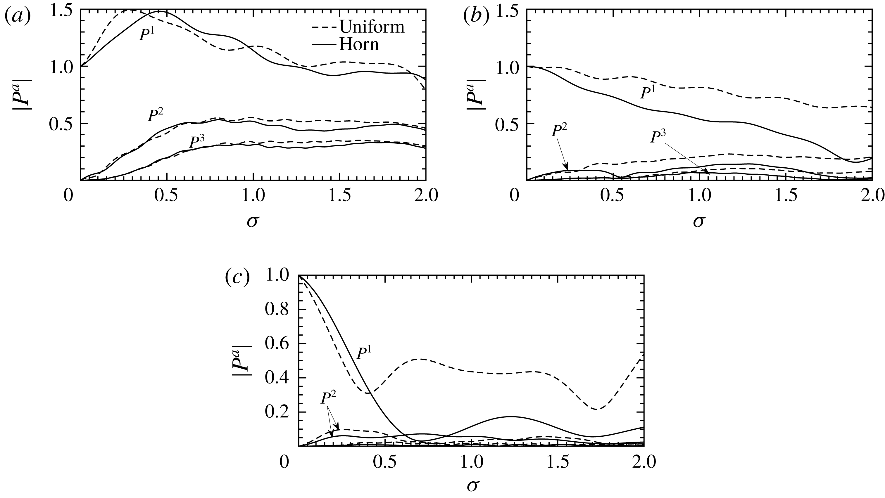
Figure 11. Comparing the modal amplitudes throughout the curved uniform duct to the curved horn along different paths.
 $M=2/(L\unicode[STIX]{x1D6FD}k)$
. (a) The outside of the bend, (b) the centre of the bend, (c) the inside of the bend.
$M=2/(L\unicode[STIX]{x1D6FD}k)$
. (a) The outside of the bend, (b) the centre of the bend, (c) the inside of the bend.
Figures 9–11 compare the modal amplitudes throughout the ducts. As previously observed, the curved duct shows a strong harmonic enrichment on the outside of the duct bend at the cost of enrichment towards the centre and inside. Therefore it would seem that the ‘observability’ of the bend in a duct system – i.e. whether one could detect if there is a bend upstream – is dependant on whether the ensuing duct can support propagation of higher spatial modes. For low frequencies or narrow ducts it would seem likely that this extra harmonic enrichment would be lost due to reflection, but for high frequencies one could expect highly enriched localised sound to propagate downstream of a bend.
For the horn we compare the pressure normalised to the square root of the duct width to account for the spreading of the waveform. The harmonic enrichment is indeed less than a straight duct, with more energy remaining in the fundamental. However, as noted before, there is the potential for more energy to escape through these nonlinear effects.
These two effects can be seen to combine when comparing the curved uniform duct and the curved horn. While the horn effect reduces enrichment for most points across the duct, the curvature focuses the sound at the outer edge such that it is of comparable amplitude to the uniform curve. As the exit width is larger for the horn, some of these more localised modes can propagate out.
To better examine the downstream effects of the varying duct shape we consider the power spectrum associated with each of the duct modes. We vary the input power of our plane wave source and find the output power of the duct for each of the spatial modes and temporal harmonics (see figure 12). For the planar modes the straight duct provides the most enrichment with the curved ducts providing significantly less. When one looks at the higher spatial modes however, one finds a similar degree of enrichment, particularly with the curved horn (which has fewer cut off modes). As an aside it is also interesting to note that modes which would traditionally be cutoff and transmit no power in a linear regime can now do so at sufficiently high Mach numbers (see
 $P_{1}^{1}$
for the uniform curved duct).
$P_{1}^{1}$
for the uniform curved duct).

Figure 12. Comparing the power outputs of the different ducts. (a) The planar modes, (b) mode 1, (c) mode 2.
7 Nonlinear reflection
As we have previously noted at several points, nonlinearity can transfer energy to higher modes and allow them to propagate in to regions where a linear wave would not. We have also observed modes which would not traditionally carry energy under a linear regime now doing so. This suggests it is important to reformulate our notions of reflection coefficients and matrices to also take into account the amplitude of the sound waves we are dealing with. We begin with the characteristic admittance relation for forward and backward propagating modes
 $$\begin{eqnarray}\boldsymbol{u}^{\pm }=\unicode[STIX]{x1D654}^{\pm }\boldsymbol{p}^{\pm }+{\mathcal{Y}}^{\pm }[\,\boldsymbol{p}^{\pm },\boldsymbol{p}^{\pm }].\end{eqnarray}$$
We now define a nonlinear reflection relation, relating forwards and backwards propagating pressure modes
 $$\begin{eqnarray}\boldsymbol{p}^{-}=\unicode[STIX]{x1D64D}\boldsymbol{p}^{+}+{\mathcal{R}}[\,\boldsymbol{p}^{+},\boldsymbol{p}^{+}],\end{eqnarray}$$
where
 $\unicode[STIX]{x1D64D}$
is the common reflection matrix encountered in the linear literature and
$\unicode[STIX]{x1D64D}$
is the common reflection matrix encountered in the linear literature and
 ${\mathcal{R}}$
is the new nonlinear reflectance, both of which vary throughout the duct. From the standard impedance relation we have
${\mathcal{R}}$
is the new nonlinear reflectance, both of which vary throughout the duct. From the standard impedance relation we have
 $$\begin{eqnarray}\boldsymbol{u}=\boldsymbol{u}^{+}+\boldsymbol{u}^{-}=\unicode[STIX]{x1D654}\boldsymbol{p}+{\mathcal{Y}}[\,\boldsymbol{p},\boldsymbol{p}]=\unicode[STIX]{x1D654}(\boldsymbol{p}^{+}+\boldsymbol{p}^{-})+{\mathcal{Y}}[\,\boldsymbol{p}^{+}+\boldsymbol{p}^{-},\boldsymbol{p}^{+}+\boldsymbol{p}^{-}].\end{eqnarray}$$
The
 $\boldsymbol{u}^{\pm }$
can be expressed in terms of
$\boldsymbol{u}^{\pm }$
can be expressed in terms of
 $\boldsymbol{p}^{\pm }$
using (7.1) and, subsequently, the
$\boldsymbol{p}^{\pm }$
using (7.1) and, subsequently, the
 $\boldsymbol{p}^{-}$
can be expressed in terms of
$\boldsymbol{p}^{-}$
can be expressed in terms of
 $\boldsymbol{p}^{+}$
using the reflection relation (7.2) to get
$\boldsymbol{p}^{+}$
using the reflection relation (7.2) to get
 $$\begin{eqnarray}\displaystyle & & \displaystyle \unicode[STIX]{x1D654}^{+}\boldsymbol{p}^{+}+{\mathcal{Y}}^{+}[\,\boldsymbol{p}^{+},\boldsymbol{p}^{+}]+\unicode[STIX]{x1D654}^{-}(\unicode[STIX]{x1D64D}\boldsymbol{p}^{+}+{\mathcal{R}}[\,\boldsymbol{p}^{+},\boldsymbol{p}^{+}])+{\mathcal{Y}}^{-}[\unicode[STIX]{x1D64D}\boldsymbol{p}^{+},\unicode[STIX]{x1D64D}\boldsymbol{p}^{+}]\nonumber\\ \displaystyle & & \displaystyle \quad =\unicode[STIX]{x1D654}(\boldsymbol{p}^{+}+\unicode[STIX]{x1D64D}\boldsymbol{p}^{+}+{\mathcal{R}}[\,\boldsymbol{p}^{+},\boldsymbol{p}^{+}])+{\mathcal{Y}}[\,\boldsymbol{p}^{+}+\unicode[STIX]{x1D64D}\boldsymbol{p}^{+},\boldsymbol{p}^{+}+\unicode[STIX]{x1D64D}\boldsymbol{p}^{+}].\end{eqnarray}$$
As with formulating our impedance relations, orders of magnitude can then be taken to form two distinct equations, and the
 $\boldsymbol{p}^{+}$
can be cancelled off. From this we obtain the usual definition of the reflection matrix
$\boldsymbol{p}^{+}$
can be cancelled off. From this we obtain the usual definition of the reflection matrix
 $$\begin{eqnarray}\unicode[STIX]{x1D64D}=(\unicode[STIX]{x1D654}-\unicode[STIX]{x1D654}^{-})^{-1}(\unicode[STIX]{x1D654}^{+}-\unicode[STIX]{x1D654})\end{eqnarray}$$
and the new nonlinear reflectance
 $$\begin{eqnarray}{\mathcal{R}}=(\unicode[STIX]{x1D654}-\unicode[STIX]{x1D654}^{-})^{-1}({\mathcal{Y}}^{+}+{\mathcal{Y}}^{-}[\unicode[STIX]{x1D64D},\unicode[STIX]{x1D64D}]-{\mathcal{Y}}[\unicode[STIX]{x1D644}+\unicode[STIX]{x1D64D},\unicode[STIX]{x1D644}+\unicode[STIX]{x1D64D}]).\end{eqnarray}$$
We can use these to obtain the reflective properties of a duct. If we have an incident wave
 $\boldsymbol{p}^{+}$
, we can calculate the power associated with such a wave
$\boldsymbol{p}^{+}$
, we can calculate the power associated with such a wave
 $$\begin{eqnarray}W^{+}=\text{Re}(\boldsymbol{p}^{+}\boldsymbol{\cdot }\overline{\boldsymbol{u}^{+}})=\text{Re}(\boldsymbol{p}^{+}\overline{\unicode[STIX]{x1D654}^{+}\boldsymbol{p}^{+}}+\boldsymbol{p}^{+}\overline{{\mathcal{Y}}^{+}}[\overline{\boldsymbol{p}^{+}},\overline{\boldsymbol{p}^{+}}]).\end{eqnarray}$$
The total pressure is given by
 $$\begin{eqnarray}\boldsymbol{p}=(\unicode[STIX]{x1D644}+\unicode[STIX]{x1D64D})\boldsymbol{p}^{+}+{\mathcal{R}}[\,\boldsymbol{p}^{+},\boldsymbol{p}^{+}].\end{eqnarray}$$
Therefore the total power is
 $$\begin{eqnarray}W=\text{Re}(\boldsymbol{p}\overline{\unicode[STIX]{x1D654}}\overline{\boldsymbol{p}}+\boldsymbol{p}\overline{{\mathcal{Y}}}[\overline{\boldsymbol{p}},\overline{\boldsymbol{p}}]).\end{eqnarray}$$
Unlike in the linear case the total energy flux is not a sum of
 $W^{+}$
and the analogous
$W^{+}$
and the analogous
 $W^{-}$
as there are nonlinear interactions. Instead we take our amplitude reflection modulus to be
$W^{-}$
as there are nonlinear interactions. Instead we take our amplitude reflection modulus to be
 $$\begin{eqnarray}R=\sqrt{\frac{W-W^{+}}{W^{+}}}.\end{eqnarray}$$
Figure 13 shows how the amount of energy reflected in the depends both on frequency of the signal and the amplitude for the uniform curved duct studied in § 5.4. Low frequencies have a much lower dependence on amplitude than higher frequencies and larger amplitudes have a much more sensitive dependence on frequency, with interesting new resonances arising. Also plotted are the experimental results of Cabelli (Reference Cabelli1980). Nonlinearity may account for the discrepancy between the experimental results and the linear multimodal method, though as no amplitude was stated one cannot be certain.
Figure 14 is a similar plot for the elephant’s trunk described in § 5.5. In this case the effects of nonlinearity have little effect on the reflection coefficient – presumably due to the decreasing width not only reflecting many of the fundamental duct modes, but also many of the modes of the temporal harmonics as well. Thus, even though the sound is enriched, it is not enriched enough to propagate down the narrow exit.
Figure 15 illustrates the opposite effect for the horn described in § 5.3. Due to the increasing width, many of the modes of the harmonics produced by spectral enrichment can propagate, whereas the fundamental modes cannot. Therefore, as noted earlier, more energy can escape the horn as the enrichment increases. This is confirmed by this graph with higher Mach numbers reducing the reflection coefficient.

Figure 13. Modulus of the reflection coefficient at various amplitudes for the uniform curved duct described in § 5.4. The ‘
 $\circ$
’ are the experimental results of Cabelli (Reference Cabelli1980).
$\circ$
’ are the experimental results of Cabelli (Reference Cabelli1980).

Figure 14. Modulus of the reflection coefficient at various amplitudes for the elephant’s trunk described in § 5.5.

Figure 15. Modulus of the reflection coefficient at various amplitudes for the elephant’s trunk described in § 5.3.
8 Conclusion
A multimodal method for the calculation of weakly nonlinear sound propagation in bends of general curvature and width has been presented. The method directly extends the linear curved-duct analysis of Félix & Pagneux (Reference Félix and Pagneux2001) into the weakly nonlinear regime, and allows for a more general arbitrarily curved-duct geometry, while reducing to their method in the infinitesimal amplitude limit. The method also extends the nonlinear straight-duct analysis of Fernando et al. (Reference Fernando, Druon, Coulouvrat and Marchiano2011) to allow for curved ducts of varying width. The method also reproduces the classical nonlinear acoustic phenomena such as wave steepening and shock formation, matching the analytical results for one dimension.
The method was applied to ducts previously studied in the linear literature, where it was shown that wave steepening can play an important role in the shape of the waveform propagating in complex geometry. A particularly important result is that nonlinear harmonic enrichment can lead to a greater transmission of sound out of an acoustic horn.
Different geometries were compared to gain an insight into how the duct shape can affect the acoustic properties in the nonlinear regime. A greater degree of wave steeping was observed on the outside of a bend when compared to a straight duct due to a greater localisation of energy. How this affects the sound radiated remains an open question, and is presently being worked on by the authors.
Two fundamental extensions to the existing linear notation have been proposed in the course of this work: the extension of linear admittance
 $\boldsymbol{u}=\unicode[STIX]{x1D654}\boldsymbol{p}$
to weakly nonlinear (2.37), and the extension of linear reflectance
$\boldsymbol{u}=\unicode[STIX]{x1D654}\boldsymbol{p}$
to weakly nonlinear (2.37), and the extension of linear reflectance
 $\boldsymbol{p}^{-}=\unicode[STIX]{x1D64D}\boldsymbol{p}^{+}$
to weakly nonlinear (7.2). The admittance (or, equivalently, the impedance) is often used as either an input or output boundary condition, dictating how much sound is allowed in or let out of a duct, and the nonlinear extension includes the effects of the wave amplitude at the boundary. The reflectance is often used as an internal boundary condition, dictating how much sound at a boundary is reflected back into the duct, and the extension to the notion of reflectance takes into account the amplitude of the incident wave. These extensions could have important consequences for the resonances in musical instruments where, for example, one may be able to calculate the change in pitch of a brass instrument with the playing volume. The nonlinear admittance could also be used to concatenate different shaped ducts to form a lumped-element model, extending linear lumped-element models to weak nonlinearity.
$\boldsymbol{p}^{-}=\unicode[STIX]{x1D64D}\boldsymbol{p}^{+}$
to weakly nonlinear (7.2). The admittance (or, equivalently, the impedance) is often used as either an input or output boundary condition, dictating how much sound is allowed in or let out of a duct, and the nonlinear extension includes the effects of the wave amplitude at the boundary. The reflectance is often used as an internal boundary condition, dictating how much sound at a boundary is reflected back into the duct, and the extension to the notion of reflectance takes into account the amplitude of the incident wave. These extensions could have important consequences for the resonances in musical instruments where, for example, one may be able to calculate the change in pitch of a brass instrument with the playing volume. The nonlinear admittance could also be used to concatenate different shaped ducts to form a lumped-element model, extending linear lumped-element models to weak nonlinearity.
The numerical implementation of the proposed method described in § 4, while practical on modest computational hardware, can nonetheless be expensive in terms of computational time and memory requirements. Two possible extensions could lead to reduced computational requirements. The first is to use the idea of Bi (Reference Bi2008) to use an overdetermined basis of functions for the spatial modal expansion, including a straight-duct mode with a Dirichlet boundary condition in addition to the basis of straight duct modes with Neumann boundary conditions, in order to more easily satisfy the boundary conditions and lead to faster convergence; for their case, Bi (Reference Bi2008) showed this accelerated convergence from
 $O(N^{-3})$
to
$O(N^{-3})$
to
 $O(N^{-5})$
, where
$O(N^{-5})$
, where
 $N$
is the number of modes included. Such an improvement in convergence rate could also be expected here. Secondly, memory requirements could be reduced at the cost of a slight increase in computational cost by checkpointing, in a similar way to calculations in adjoint looping. This would involve, when solving (2.42a
) and (2.42b
) for the linear and nonlinear admittance, only storing the admittances at a few axial locations rather than at all calculated locations along the duct, with a significant memory saving. Subsequently, when the admittances are needed to solve (2.44) for the pressure within the duct, the admittances would be re-calculated by re-solving (2.42a
) and (2.42b
) from the nearest stored values of the admittances. Whether this tradeoff between extra computational expense and reduced memory requirements is advantageous would be parameter dependent.
$N$
is the number of modes included. Such an improvement in convergence rate could also be expected here. Secondly, memory requirements could be reduced at the cost of a slight increase in computational cost by checkpointing, in a similar way to calculations in adjoint looping. This would involve, when solving (2.42a
) and (2.42b
) for the linear and nonlinear admittance, only storing the admittances at a few axial locations rather than at all calculated locations along the duct, with a significant memory saving. Subsequently, when the admittances are needed to solve (2.44) for the pressure within the duct, the admittances would be re-calculated by re-solving (2.42a
) and (2.42b
) from the nearest stored values of the admittances. Whether this tradeoff between extra computational expense and reduced memory requirements is advantageous would be parameter dependent.
The examples given in this paper are either taken from existing literature for comparative purposes, or are designed purely to be taxing test cases which demonstrate a range of interesting behaviours. Whilst one promising possible application of this work is in the analysis of brass instruments (e.g. Gilbert et al. Reference Gilbert, Menguy and Campbell2008; Rendón et al. Reference Rendón, Orduña-Bustamante, Narezo, Pérez-López and Sorrentini2010), it is not clear whether the features seen in the examples given here are indicative of behaviour in actual brass instruments, and further study would be needed. In particular, the exponential horn is not particularly representative of brass instrument bells, for which the degree of flaring is an important feature of the instrument’s design; such features could be investigated using the method presented here, although to accurately model an open duct end and propagation to the far field the weakly nonlinear admittance at an open duct end would need to be derived, accounting for weakly nonlinear effects in the near field outside the duct.
Work is also currently under way extending this method to fully three-dimensional ducts (including those with torsion) to which a richer degree of phenomena are possible.
Acknowledgements
J.P.M. gratefully acknowledges the support of an EPSRC Doctoral Training Grant. E.J.B. gratefully acknowledges the support of a Royal Society University Research Fellowship (UF150695).
Appendix A. Modes of zero frequency
In this appendix we justify ignoring the modes of zero frequency. From (2.14a
), setting
 $a=0$
we obtain
$a=0$
we obtain
 $$\begin{eqnarray}\unicode[STIX]{x1D735}\boldsymbol{\cdot }\boldsymbol{U}^{0}=\mathop{\sum }_{b=-\infty }^{\infty }(-\text{i}bkP^{-b}P^{b}-\text{i}bkU^{-b}U^{b}-\text{i}bkV^{-b}V^{b}),\end{eqnarray}$$
where we have substituted for the differential terms on the right-hand side. It can clearly be seen that upon summation, the right-hand side vanishes and we are left with the classical incompressibility condition
 $\unicode[STIX]{x1D735}\boldsymbol{\cdot }\boldsymbol{U}^{0}=0$
. As such, the modes
$\unicode[STIX]{x1D735}\boldsymbol{\cdot }\boldsymbol{U}^{0}=0$
. As such, the modes
 $U^{0}$
are decoupled from the acoustic modes and we do not have acoustic streaming. As we are not imposing any mean flow in the duct and none is induced by the acoustic phenomena, we ignore the modes
$U^{0}$
are decoupled from the acoustic modes and we do not have acoustic streaming. As we are not imposing any mean flow in the duct and none is induced by the acoustic phenomena, we ignore the modes
 $U^{0}$
.
$U^{0}$
.
By taking (2.18a
) and (2.18c
), and the linear relationship between
 $P^{a}$
and
$P^{a}$
and
 $U^{a}$
given by (2.30), it can be seen that (2.14b
) reduces to
$U^{a}$
given by (2.30), it can be seen that (2.14b
) reduces to
 $$\begin{eqnarray}\unicode[STIX]{x1D735}P^{0}=-\mathop{\sum }_{b=-\infty }^{\infty }\unicode[STIX]{x1D735}\left(\frac{1}{2}U^{-b}U^{b}-\frac{1}{2}P^{-b}P^{b}\right)\end{eqnarray}$$
for
 $a=0$
. Therefore we have
$a=0$
. Therefore we have
 $$\begin{eqnarray}P^{0}=-\langle {\mathcal{L}}\rangle ,\end{eqnarray}$$
where
 ${\mathcal{L}}=\hat{\boldsymbol{u}}^{2}/2-\hat{p}^{2}/2$
is the Lagrangian density of energy and
${\mathcal{L}}=\hat{\boldsymbol{u}}^{2}/2-\hat{p}^{2}/2$
is the Lagrangian density of energy and
 $\langle \,\rangle$
denotes time average. As this is an order of magnitude smaller than the other pressure terms (noting that while we have retained terms of
$\langle \,\rangle$
denotes time average. As this is an order of magnitude smaller than the other pressure terms (noting that while we have retained terms of
 $\mathit{O}(M^{2})$
in our equations, their effect is cumulative whereas the local sound pressure we are interested in is
$\mathit{O}(M^{2})$
in our equations, their effect is cumulative whereas the local sound pressure we are interested in is
 $\mathit{O}(M)$
), it does not affect our governing equations. It can therefore be ignored in calculations and makes little difference to the final pressure profile.
$\mathit{O}(M)$
), it does not affect our governing equations. It can therefore be ignored in calculations and makes little difference to the final pressure profile.
Appendix B. Analytic expressions for the
$\unicode[STIX]{x1D733}$
matrices

 $$\begin{eqnarray}\displaystyle \unicode[STIX]{x1D733}_{pq} & = & \displaystyle \unicode[STIX]{x1D6FF}_{pq},\end{eqnarray}$$
 $$\begin{eqnarray}\displaystyle \unicode[STIX]{x1D733}_{[\,p]q} & = & \displaystyle \left\{\begin{array}{@{}ll@{}}C_{p}C_{q}{\displaystyle \frac{p^{2}((-1)^{p+q}-1)}{p^{2}-q^{2}}}\quad & p\neq q\\ 0\quad & p=q\end{array}\right.,\end{eqnarray}$$
 $$\begin{eqnarray}\displaystyle \unicode[STIX]{x1D733}_{pq}[r] & = & \displaystyle \left\{\begin{array}{@{}ll@{}}C_{p}C_{q}{\displaystyle \frac{(p^{2}+q^{2})(h_{+}-h_{-})^{2}((-1)^{p+q}-1)}{\unicode[STIX]{x03C0}^{2}(p^{2}-q^{2})^{2}}}\quad & p\neq q\\ (h_{+}+h_{-})/2\quad & p=q\end{array}\right.,\end{eqnarray}$$
 $$\begin{eqnarray}\displaystyle \unicode[STIX]{x1D733}_{[\,p]q}[r] & = & \displaystyle \left\{\begin{array}{@{}ll@{}}C_{p}C_{q}{\displaystyle \frac{p^{2}(h_{+}(-1)^{p+q}-h_{-})}{p^{2}-q^{2}}}\quad & p\neq q\\ 1/2\quad & p=q,\quad p\neq 0,\\ 0\quad & p=0,\end{array}\right.\end{eqnarray}$$
 $$\begin{eqnarray}\displaystyle \unicode[STIX]{x1D733}_{\{p\}q} & = & \displaystyle \left\{\begin{array}{@{}ll@{}}-\left({\displaystyle \frac{h_{+}^{\prime }-h_{-}^{\prime }}{h_{+}-h_{-}}}\right)(1-\unicode[STIX]{x1D6FF}_{p0}/2)\quad & p=q\\ -C_{p}C_{q}((-1)^{p+q}h_{+}^{\prime }-h_{-}^{\prime }){\displaystyle \frac{p^{2}}{p^{2}-q^{2}}}\quad & p\neq q\end{array}\right.,\end{eqnarray}$$
 $$\begin{eqnarray}\displaystyle \unicode[STIX]{x1D733}_{pqr} & = & \displaystyle C_{p}C_{q}C_{r}{\displaystyle \frac{(h_{+}-h_{-})}{4}}(\unicode[STIX]{x1D6FF}_{p,q+r}+\unicode[STIX]{x1D6FF}_{p,|q-r|}+\unicode[STIX]{x1D6FF}_{p,0}\unicode[STIX]{x1D6FF}_{q,r}+\unicode[STIX]{x1D6FF}_{p,0}\unicode[STIX]{x1D6FF}_{q,0}\unicode[STIX]{x1D6FF}_{r,0}),\end{eqnarray}$$
 $$\begin{eqnarray}\displaystyle \unicode[STIX]{x1D733}_{[\,p]qr} & = & \displaystyle \left\{\begin{array}{@{}ll@{}}C_{p}C_{q}C_{r}{\displaystyle \frac{p^{2}((-1)^{p+q+r}-1)(p^{2}-q^{2}-r^{2})}{(p+q+r)(p+q-r)(p-q+r)(p-q-r)}}\quad \\ \qquad p\neq |q+r|,\quad p\neq |q-r|\quad \\ 0\quad & \text{else},\end{array}\right.\end{eqnarray}$$
 $$\begin{eqnarray}\displaystyle \unicode[STIX]{x1D733}_{pqr}[r] & = & \displaystyle \left\{\begin{array}{@{}ll@{}}C_{p}C_{q}C_{r}((-1)^{p+q+r}-1){\displaystyle \frac{(h_{+}-h_{-})^{2}}{4\unicode[STIX]{x03C0}^{2}}}\left(\vphantom{{\displaystyle \frac{1}{(p-q-r)^{2}}}}\ldots {\displaystyle \frac{1}{(p+q+r)^{2}}}\right.\quad & \\ \quad +\left.{\displaystyle \frac{1}{(p-q+r)^{2}}}+{\displaystyle \frac{1}{(p+q-r)^{2}}}+{\displaystyle \frac{1}{(p-q-r)^{2}}}\right)\quad & p\neq |q+r|,\\ \quad & p\neq |q-r|\\ 0\quad & \text{else}\end{array}\right.\nonumber\\ \displaystyle & & \displaystyle\end{eqnarray}$$
 $$\begin{eqnarray}\displaystyle \unicode[STIX]{x1D733}_{[\,p]qr}[r] & = & \displaystyle \left\{\begin{array}{@{}ll@{}}C_{p}C_{q}C_{r}{\displaystyle \frac{(h_{+}(-1)^{p+q+r}-h_{-})p^{2}(p^{2}-q^{2}-r^{2})}{(p+q+r)(p+q-r)(p-q+r)(p-q-r)}}\quad & \\ \qquad p\notin \{|q+r|,\,|q-r|\},\quad \\ {\displaystyle \frac{C_{p}C_{q}C_{r}}{8}}(h_{+}-h_{-})p\left({\displaystyle \frac{1}{q+r}}+{\displaystyle \frac{1}{q}}+{\displaystyle \frac{1}{r}}\right),\quad & p=q+r,\\ {\displaystyle \frac{C_{p}C_{q}C_{r}}{8}}(h_{+}-h_{-})p\left({\displaystyle \frac{1}{q}}-{\displaystyle \frac{1}{r}}+{\displaystyle \frac{1}{q-r}}\right),\quad & p=q-r,\\ {\displaystyle \frac{C_{p}C_{q}C_{r}}{8}}(h_{+}-h_{-})p\left({\displaystyle \frac{1}{r}}-{\displaystyle \frac{1}{r}}+{\displaystyle \frac{1}{r-q}}\right),\quad & p=r-q,\\ {\displaystyle \frac{C_{p}C_{q}C_{r}}{4}}(h_{+}-h_{-}),\quad & p=q,r=0,\\ {\displaystyle \frac{C_{p}C_{q}C_{r}}{4}}(h_{+}-h_{-}),\quad & p=r,q=0,\\ 0,\quad & \text{else},\end{array}\right.\nonumber\\ \displaystyle & & \displaystyle\end{eqnarray}$$
 $$\begin{eqnarray}\displaystyle \unicode[STIX]{x1D733}_{\{p\}qr} & = & \displaystyle -{\displaystyle \frac{(h_{+}^{\prime }-h_{-}^{\prime })}{2(h_{+}-h_{-})}}\unicode[STIX]{x1D733}_{pqr}+{\displaystyle \frac{h_{-}h_{+}^{\prime }-h_{+}h_{-}^{\prime }}{h_{+}-h_{-}}}\unicode[STIX]{x1D733}_{[\,p]qr}-{\displaystyle \frac{h_{+}^{\prime }-h_{-}^{\prime }}{h_{+}-h_{-}}}\unicode[STIX]{x1D733}_{[\,p]qr}[r],\end{eqnarray}$$
 $$\begin{eqnarray}\displaystyle {\displaystyle \frac{\unicode[STIX]{x2202}}{\unicode[STIX]{x2202}s}}(\unicode[STIX]{x1D733}_{pqr}) & = & \displaystyle -{\displaystyle \frac{1}{2}}\left({\displaystyle \frac{h_{+}^{\prime }-h_{-}^{\prime }}{h_{+}-h_{-}}}\right)\unicode[STIX]{x1D733}_{pqr}.\end{eqnarray}$$
Appendix C. Equivalence to the Fubini and sawtooth solutions
The case of nonlinear sound propagation in one dimension has been much studied. The Fubini solution (Fubini Reference Fubini1935), which is valid up to the point of shock formation, gives the harmonic amplitudes of pressure for a sinusoidal pressure source propagating in one dimension. The modal amplitudes,
 $B_{a}$
are given by
$B_{a}$
are given by
 $$\begin{eqnarray}B_{a}={\displaystyle \frac{2}{a\unicode[STIX]{x1D70E}}}J_{a}(a\unicode[STIX]{x1D70E}).\end{eqnarray}$$
In our notation, this corresponds to a solution
 $$\begin{eqnarray}P_{0}^{a}=\text{i}M\sqrt{h_{+}-h_{-}}{\displaystyle \frac{1}{a\unicode[STIX]{x1D70E}}}J_{a}(a\unicode[STIX]{x1D70E})\text{e}^{\text{i}aks},\end{eqnarray}$$
where the factor of
 $\text{i}$
in the front ensures the solution satisfies
$\text{i}$
in the front ensures the solution satisfies
 $P^{-a}=(P^{a})^{\ast }$
.
$P^{-a}=(P^{a})^{\ast }$
.
In one dimension, equation (2.44) can be heavily simplified. Both the linear and nonlinear parts of the admittance are given by their characteristic forms for a straight duct
 $$\begin{eqnarray}\unicode[STIX]{x1D654}^{a}=1,\quad {\mathcal{Y}}^{ab}=-{\displaystyle \frac{\unicode[STIX]{x1D6FD}}{2\sqrt{h_{+}-h_{-}}}}.\end{eqnarray}$$
Thus, equation (2.44) reduces to
 $$\begin{eqnarray}{\displaystyle \frac{\text{d}}{\text{d}s}}P^{a}=\text{i}akP^{a}-\mathop{\sum }_{b=-\infty }^{\infty }\left({\displaystyle \frac{\text{i}ak\unicode[STIX]{x1D6FD}}{2\sqrt{h_{+}-h_{-}}}}P^{a-b}P^{b}+{\displaystyle \frac{\text{i}(a-2b)k}{\sqrt{h_{+}-h_{-}}}}P^{a-b}P^{b}\right).\end{eqnarray}$$
The third term in this equation – corresponding to
 ${\mathcal{C}}[\mathsf{Y}\boldsymbol{p},\boldsymbol{p}]$
in (2.44) – may be written
${\mathcal{C}}[\mathsf{Y}\boldsymbol{p},\boldsymbol{p}]$
in (2.44) – may be written
 $$\begin{eqnarray}{\displaystyle \frac{\text{i}k}{\sqrt{h_{+}-h_{-}}}}((a-b)-b)P^{a-b}P^{b}\end{eqnarray}$$
and hence vanishes on summation. This happens because the term
 ${\mathcal{C}}$
corresponds to the Lagrangian density of energy, which vanishes for plane waves (Hamilton & Blackstock Reference Hamilton and Blackstock1990). We are therefore left with
${\mathcal{C}}$
corresponds to the Lagrangian density of energy, which vanishes for plane waves (Hamilton & Blackstock Reference Hamilton and Blackstock1990). We are therefore left with
 $$\begin{eqnarray}{\displaystyle \frac{\text{d}}{\text{d}s}}P^{a}=\text{i}akP^{a}-{\displaystyle \frac{\text{i}ak\unicode[STIX]{x1D6FD}}{2\sqrt{h_{+}-h_{-}}}}P^{a-b}P^{b}.\end{eqnarray}$$
Upon substituting (C 2) into (C 6) we are left with
 $$\begin{eqnarray}{\displaystyle \frac{1}{\unicode[STIX]{x1D70E}}}J_{a}^{\prime }(a\unicode[STIX]{x1D70E})-{\displaystyle \frac{1}{a\unicode[STIX]{x1D70E}^{2}}}J_{a}(a\unicode[STIX]{x1D70E})=\mathop{\sum }_{b=-\infty }^{\infty }{\displaystyle \frac{a}{2(a-b)b}}J_{a-b}((a-b)\unicode[STIX]{x1D70E})J_{b}(b\unicode[STIX]{x1D70E}).\end{eqnarray}$$
Based upon numerical evaluations, this appears to be a Bessel identity valid for
 $\unicode[STIX]{x1D70E}<1$
. Under this assumption the Fubini solution is a solution to our equations up to shock formation.
$\unicode[STIX]{x1D70E}<1$
. Under this assumption the Fubini solution is a solution to our equations up to shock formation.
For
 $\unicode[STIX]{x1D70E}>3$
the waveform assumes a sawtooth shape (Blackstock Reference Blackstock1966). The solution in this region (corresponding to the Fay (Reference Fay1931) solution in the lossless limit) is given by
$\unicode[STIX]{x1D70E}>3$
the waveform assumes a sawtooth shape (Blackstock Reference Blackstock1966). The solution in this region (corresponding to the Fay (Reference Fay1931) solution in the lossless limit) is given by
 $$\begin{eqnarray}P^{a}={\displaystyle \frac{\text{i}M\sqrt{h_{+}-h_{-}}}{(1+\unicode[STIX]{x1D70E})a}}\text{e}^{\text{i}aks}.\end{eqnarray}$$
In (C 6) we get
 $$\begin{eqnarray}-{\displaystyle \frac{1}{a}}{\displaystyle \frac{\text{i}\unicode[STIX]{x1D6FD}kM^{2}\sqrt{h_{+}-h_{-}}}{(1+\unicode[STIX]{x1D70E})^{2}}}\text{e}^{\text{i}aks}=\mathop{\sum }_{b=-\infty }^{\infty }{\displaystyle \frac{a}{2(a-b)b}}{\displaystyle \frac{\text{i}\unicode[STIX]{x1D6FD}kM^{2}\sqrt{h_{+}-h_{-}}}{(1+\unicode[STIX]{x1D70E})^{2}}}\text{e}^{\text{i}aks}.\end{eqnarray}$$
The right-hand side factor can be split into partial fractions
 $$\begin{eqnarray}\displaystyle \mathop{\sum }_{b=-\infty }^{\infty }{\displaystyle \frac{a}{2(a-b)b}} & = & \displaystyle {\displaystyle \frac{1}{2}}\mathop{\sum }_{b=-\infty }^{\infty }\left({\displaystyle \frac{1}{a-b}}+{\displaystyle \frac{1}{b}}\right)\nonumber\\ \displaystyle & = & \displaystyle {\displaystyle \frac{1}{2}}\mathop{\sum }_{b=1}^{a-1}\left({\displaystyle \frac{1}{a-b}}+{\displaystyle \frac{1}{b}}\right)+{\displaystyle \frac{1}{2}}\mathop{\sum }_{b=1}^{\infty }\left({\displaystyle \frac{1}{a+b}}-{\displaystyle \frac{1}{b}}\right)\nonumber\\ \displaystyle & & \displaystyle +\,{\displaystyle \frac{1}{2}}\mathop{\sum }_{b=a+1}^{\infty }\left(-{\displaystyle \frac{1}{b-a}}+{\displaystyle \frac{1}{b}}\right)\nonumber\\ \displaystyle & = & \displaystyle {\displaystyle \frac{1}{2}}\mathop{\sum }_{b=1}^{a-1}\left({\displaystyle \frac{1}{a-b}}+{\displaystyle \frac{1}{b}}\right)+\mathop{\sum }_{b=1}^{\infty }\left({\displaystyle \frac{1}{a+b}}-{\displaystyle \frac{1}{b}}\right)\nonumber\\ \displaystyle & = & \displaystyle {\displaystyle \frac{1}{2}}\mathop{\sum }_{b=1}^{a-1}\left({\displaystyle \frac{1}{a-b}}-{\displaystyle \frac{1}{b}}\right)-{\displaystyle \frac{1}{a}}\nonumber\\ \displaystyle & = & \displaystyle -{\displaystyle \frac{1}{a}}.\end{eqnarray}$$
Thus, the sawtooth wave is a solution to the equation.
Appendix D. Uniform straight ducts
Now we consider a 2-D duct with no curvature or varying width. This was dealt with by Fernando et al. (Reference Fernando, Druon, Coulouvrat and Marchiano2011). We will now partly demonstrate the equivalence of our method and theirs. We first simplify some of the
 $\unicode[STIX]{x1D733}$
matrix products in our definitions of the matrices and tensors.
$\unicode[STIX]{x1D733}$
matrix products in our definitions of the matrices and tensors.
 $$\begin{eqnarray}\unicode[STIX]{x1D733}_{[\,p]s}\unicode[STIX]{x1D733}_{s[q]}=\mathop{\sum }_{{s=0\atop s\neq p,q}}^{\infty }C_{p}C_{q}{\displaystyle \frac{2-\unicode[STIX]{x1D6FF}_{s0}}{h_{+}-h_{-}}}p^{2}q^{2}{\displaystyle \frac{((-1)^{p+q}-(-1)^{p+s}-(-1)^{q+s}+1)}{(p^{2}-s^{2})(q^{2}-s^{2})}}.\end{eqnarray}$$
For
 $p=q$
this becomes
$p=q$
this becomes
 $$\begin{eqnarray}\unicode[STIX]{x1D733}_{[\,p]s}\unicode[STIX]{x1D733}_{s[\,p]}=\mathop{\sum }_{{s=0\atop s\neq p}}{\displaystyle \frac{2-\unicode[STIX]{x1D6FF}_{s0}}{(h_{+}-h_{-})^{2}}}(1-(-1)^{p+s})\left({\displaystyle \frac{p^{2}}{(s-p)^{2}}}+{\displaystyle \frac{p^{2}}{(p+s)^{2}}}-{\displaystyle \frac{p}{s-p}}+{\displaystyle \frac{p}{s+p}}\right)\end{eqnarray}$$
and the terms with numerator linear in
 $p$
cancel upon summation. The terms with numerator quadratic in
$p$
cancel upon summation. The terms with numerator quadratic in
 $p$
correspond to the sum
$p$
correspond to the sum
 $\sum _{s=odd}(8p^{2}/s^{2})=p^{2}\unicode[STIX]{x03C0}^{2}$
after rearrangement. For
$\sum _{s=odd}(8p^{2}/s^{2})=p^{2}\unicode[STIX]{x03C0}^{2}$
after rearrangement. For
 $p\neq q$
 $$\begin{eqnarray}\displaystyle \unicode[STIX]{x1D733}_{[\,p]s}\unicode[STIX]{x1D733}_{s[q]} & = & \displaystyle \mathop{\sum }_{{s=0\atop s\neq p,q}}^{\infty }C_{p}C_{q}{\displaystyle \frac{2-\unicode[STIX]{x1D6FF}_{s0}}{h_{+}-h_{-}}}((-1)^{p+q}-(-1)^{p+s}-(-1)^{q+s}+1)\nonumber\\ \displaystyle & & \displaystyle \times \,\left({\displaystyle \frac{p^{2}q}{2(p-q)(p+q)(q+s)}}-{\displaystyle \frac{p^{2}q}{2(p-q)(p+q)(s-q)}}\right.\nonumber\\ \displaystyle & & \displaystyle +\left.{\displaystyle \frac{pq^{2}}{2(p-q)(p+q)(s-p)}}-{\displaystyle \frac{pq^{2}}{2(p-q)(p+q)(p+s)}}\right)\end{eqnarray}$$
and it can be seen that the pairs of partial fractions cancel out upon summation. Hence we are left with
 $$\begin{eqnarray}\unicode[STIX]{x1D733}_{[\,p]s}\unicode[STIX]{x1D733}_{s[q]}=\unicode[STIX]{x1D6FF}_{pq}{\displaystyle \frac{p^{2}\unicode[STIX]{x03C0}^{2}}{(h_{+}-h_{-})^{2}}}=\unicode[STIX]{x1D6FF}_{pq}\unicode[STIX]{x1D702}_{p}^{2}.\end{eqnarray}$$
Therefore, in a straight duct we have
 $$\begin{eqnarray}\unicode[STIX]{x1D649}_{pq}^{a}=\text{i}ak\unicode[STIX]{x1D6FF}_{pq},\quad \unicode[STIX]{x1D648}_{pq}^{a}={\displaystyle \frac{1}{\text{i}ak}}(k_{p}^{a})^{2}\unicode[STIX]{x1D6FF}_{pq}.\end{eqnarray}$$
The matrix multiplications defining the tensors can also be simplified, which is made easier by the index notation used here. For example,
 $\unicode[STIX]{x1D733}_{[\,p]s}\unicode[STIX]{x1D733}_{sqt}\unicode[STIX]{x1D733}_{t[r]}=\unicode[STIX]{x1D733}_{[\,p]qt}\unicode[STIX]{x1D733}_{t[r]}=\unicode[STIX]{x1D733}_{[\,p]q[r]}$
. We also have
$\unicode[STIX]{x1D733}_{[\,p]s}\unicode[STIX]{x1D733}_{sqt}\unicode[STIX]{x1D733}_{t[r]}=\unicode[STIX]{x1D733}_{[\,p]qt}\unicode[STIX]{x1D733}_{t[r]}=\unicode[STIX]{x1D733}_{[\,p]q[r]}$
. We also have
 $\unicode[STIX]{x1D733}_{[\,p]s}\unicode[STIX]{x1D733}_{[s]qr}=-\unicode[STIX]{x1D702}_{p}^{2}\unicode[STIX]{x1D733}_{pqr}$
and
$\unicode[STIX]{x1D733}_{[\,p]s}\unicode[STIX]{x1D733}_{[s]qr}=-\unicode[STIX]{x1D702}_{p}^{2}\unicode[STIX]{x1D733}_{pqr}$
and
 $\unicode[STIX]{x1D733}_{[\,p]q[r]}+\unicode[STIX]{x1D733}_{[\,p][q]r}=\unicode[STIX]{x1D702}_{p}^{2}\unicode[STIX]{x1D733}_{p[q][r]}$
. The tensors simplify to
$\unicode[STIX]{x1D733}_{[\,p]q[r]}+\unicode[STIX]{x1D733}_{[\,p][q]r}=\unicode[STIX]{x1D702}_{p}^{2}\unicode[STIX]{x1D733}_{p[q][r]}$
. The tensors simplify to
 $$\begin{eqnarray}\displaystyle {\mathcal{A}}_{pqr}^{ab} & = & \displaystyle -\text{i}bk\unicode[STIX]{x1D733}_{pqr}+{\displaystyle \frac{1}{2\text{i}ak}}\unicode[STIX]{x1D702}_{p}^{2}\unicode[STIX]{x1D733}_{pqr}\nonumber\\ \displaystyle & {\sim} & \displaystyle {\displaystyle \frac{1}{2\text{i}ak}}(a^{2}k^{2}+\unicode[STIX]{x1D702}_{p}^{2})\unicode[STIX]{x1D733}_{pqr},\end{eqnarray}$$
 $$\begin{eqnarray}\displaystyle {\mathcal{B}}_{pqr}^{ab} & = & \displaystyle -\left(\text{i}bk+\text{i}ak{\displaystyle \frac{B}{2A}}\right)\unicode[STIX]{x1D733}_{pqr}-{\displaystyle \frac{1}{\text{i}(a-b)k}}\unicode[STIX]{x1D733}_{p[q][r]}\nonumber\\ \displaystyle & & \displaystyle -\,{\displaystyle \frac{1}{2k^{2}(a-b)b}}{\displaystyle \frac{\unicode[STIX]{x1D702}_{p}^{2}}{\text{i}ak}}\unicode[STIX]{x1D733}_{p[q][r]}-{\displaystyle \frac{1}{\text{i}ak}}\unicode[STIX]{x1D733}_{[\,p]q[r]}\nonumber\\ \displaystyle & {\sim} & \displaystyle -\text{i}ak{\displaystyle \frac{B}{2A}}\unicode[STIX]{x1D733}_{pqr}-{\displaystyle \frac{\text{i}ak}{2}}\unicode[STIX]{x1D733}_{pqr}-{\displaystyle \frac{a^{2}k^{2}}{2\text{i}ab(b-a)k^{3}}}\unicode[STIX]{x1D733}_{p[q][r]}\nonumber\\ \displaystyle & & \displaystyle -\,{\displaystyle \frac{\unicode[STIX]{x1D702}_{p}^{2}}{2\text{i}ab(a-b)k^{3}}}\unicode[STIX]{x1D733}_{p[q][r]}-{\displaystyle \frac{\unicode[STIX]{x1D702}_{p}^{2}}{2\text{i}ak}}\unicode[STIX]{x1D733}_{p[q][r]},\end{eqnarray}$$
 $$\begin{eqnarray}\displaystyle {\mathcal{C}}_{pqr}^{ab} & = & \displaystyle \text{i}ak\unicode[STIX]{x1D733}_{pqr}+{\displaystyle \frac{1}{\text{i}bk}}\unicode[STIX]{x1D733}_{[\,p]q[r]}+{\displaystyle \frac{2(k_{r}^{b})^{2}}{\text{i}bk}}\unicode[STIX]{x1D733}_{pqr},\end{eqnarray}$$
 ${\sim}$
’ denotes an equivalence relation between two tensors that, while not equal, are equivalent under summation. Because of this property it can be seen that the expressions for the tensors relating second-order quantities are not unique, but do form an equivalence class under summation. Here we have expressed
${\sim}$
’ denotes an equivalence relation between two tensors that, while not equal, are equivalent under summation. Because of this property it can be seen that the expressions for the tensors relating second-order quantities are not unique, but do form an equivalence class under summation. Here we have expressed
 ${\mathcal{A}}$
and
${\mathcal{A}}$
and
 ${\mathcal{B}}$
in a form symmetric on interchange of
${\mathcal{B}}$
in a form symmetric on interchange of
 $b\leftrightarrow (a-b)$
with
$b\leftrightarrow (a-b)$
with
 $q\leftrightarrow r$
. Having this property is sufficient to uniquely define the second-order quantities.
$q\leftrightarrow r$
. Having this property is sufficient to uniquely define the second-order quantities. The equation used by Fernando et al. (Reference Fernando, Druon, Coulouvrat and Marchiano2011) is for the velocity potential
 $\hat{\boldsymbol{u}}=\unicode[STIX]{x1D735}\hat{\unicode[STIX]{x1D719}}$
. The velocity potential is expanded about the basis of modes, with the modal amplitudes
$\hat{\boldsymbol{u}}=\unicode[STIX]{x1D735}\hat{\unicode[STIX]{x1D719}}$
. The velocity potential is expanded about the basis of modes, with the modal amplitudes
 $A_{p}^{a}$
given by
$A_{p}^{a}$
given by
 $$\begin{eqnarray}\unicode[STIX]{x1D719}_{p}^{a}=A_{p}^{a}(s)\text{e}^{\text{i}k_{p}^{a}s},\end{eqnarray}$$
where
 $A_{p}^{a}(s)$
is assumed to be
$A_{p}^{a}(s)$
is assumed to be
 $\mathit{O}(M)$
with
$\mathit{O}(M)$
with
 $\mathit{O}(M^{2})$
derivatives. The factor
$\mathit{O}(M^{2})$
derivatives. The factor
 $$\begin{eqnarray}k_{p}^{a}=\left\{\begin{array}{@{}ll@{}}(a^{2}k^{2}-\unicode[STIX]{x1D702}_{p}^{2})^{1/2},\quad & ak>\unicode[STIX]{x1D702}_{p},\quad a>0,\\ -(a^{2}k^{2}-\unicode[STIX]{x1D702}_{p}^{2})^{1/2},\quad & ak>\unicode[STIX]{x1D702}_{p},\quad a<0,\\ \text{i}(\unicode[STIX]{x1D702}_{p}^{2}-a^{2}k^{2})^{1/2},\quad & ak<\unicode[STIX]{x1D702}_{p},\end{array}\right.\end{eqnarray}$$
corresponds to the transverse wavenumber for each mode.
Note that while it may be more natural to work with the velocity potential (for example a second-order wave equation, the Kuznetzov equation (Kuznetsov Reference Kuznetsov1971), can be formed from just this variable), there is the implicit assumption of zero vorticity when using this variable – something which cannot be assumed a priori for a curved duct.
In terms of the velocity potential, the pressure is given by
 $$\begin{eqnarray}\hat{p}=-{\displaystyle \frac{1}{c_{0}}}{\displaystyle \frac{\unicode[STIX]{x2202}\hat{\unicode[STIX]{x1D719}}}{\unicode[STIX]{x2202}t}}-{\displaystyle \frac{1}{2}}\left((\unicode[STIX]{x1D735}\hat{\unicode[STIX]{x1D719}})^{2}-{\displaystyle \frac{1}{c_{0}^{2}}}\left({\displaystyle \frac{\unicode[STIX]{x2202}\hat{\unicode[STIX]{x1D719}}}{\unicode[STIX]{x2202}t}}\right)^{2}\right),\end{eqnarray}$$
corresponding to modal amplitudes given by
 $$\begin{eqnarray}P_{p}^{a}=\text{i}akA_{p}^{a}\text{e}^{\text{i}k_{p}^{a}s}+{\textstyle \frac{1}{2}}(k_{q}^{a-b}k_{r}^{b}\unicode[STIX]{x1D733}_{pqr}-\unicode[STIX]{x1D733}_{p[q][r]}-(a-b)bk^{2}\unicode[STIX]{x1D733}_{pqr})A_{q}^{a-b}A_{r}^{b}\text{e}^{\text{i}(k_{q}^{a-b}+k_{r}^{b})s}.\end{eqnarray}$$
In order to completely prove the equivalence of our method with that of Fernando et al. (Reference Fernando, Druon, Coulouvrat and Marchiano2011), one would need to derive (D 10) from a nonlinear impedance relationship analogous to (2.37). Because of the large class of equivalent tensors relating second-order quantities this has proved difficult so far.
The expression for the velocity modes is
 $$\begin{eqnarray}U_{p}^{a}=((A_{p}^{a})^{\prime }+\text{i}k_{p}^{a}A_{p}^{a})\text{e}^{\text{i}k_{p}^{a}s}.\end{eqnarray}$$
We substitute these expressions into (2.33a
) (with the above straight-duct simplifications), and, after cancellation and neglecting the second derivative of
 $A$
(for the second derivative is
$A$
(for the second derivative is
 $\mathit{O}(M^{3})$
) we obtain
$\mathit{O}(M^{3})$
) we obtain
 $$\begin{eqnarray}2k_{p}^{a}(A_{p}^{a})^{\prime }\text{e}^{\text{i}k_{p}^{a}s}=ak\left(k_{q}^{a-b}k_{r}^{b}\unicode[STIX]{x1D733}_{pqr}-\unicode[STIX]{x1D733}_{p[q][r]}+k^{2}(a-b)b{\displaystyle \frac{B}{2A}}\unicode[STIX]{x1D733}_{pqr}\right)A_{q}^{a-b}A_{r}^{b}\text{e}^{\text{i}(k_{q}^{a-b}+k_{r}^{b})s}.\end{eqnarray}$$
This is the equation presented by Fernando et al. (Reference Fernando, Druon, Coulouvrat and Marchiano2011) (in dimensionless variables with normalised modes). Solving this equation has some disadvantages over our method. Firstly, this method can only be used for forward propagating waves. With a suitable choice of admittance one can solve for the nonlinear interaction of both forward and backward propagating waves together. Secondly, for numerical stability, one must discard evanescent modes from the calculation because of the problems associated with defining an amplitude for an exponentially small mode. In our method this is not necessary – indeed, as shown by Félix & Pagneux (Reference Félix and Pagneux2001), the evanescent modes are important when one considers a duct with curvature.
As stated previously, this is not a complete proof of equivalence – one can instead refer to § 5.2 for a numerical verification.
Appendix E. Linear acoustics in a non-uniform straight duct
If we ignore the quadratic terms and terms corresponding to curvature, our equations reduce to
 $$\begin{eqnarray}\displaystyle {U_{p}^{a}}^{\prime }+{\displaystyle \frac{1}{\text{i}ak}}(k_{p}^{a})^{2}P_{p}^{a}-\unicode[STIX]{x1D733}_{\{p\}q}U_{q}^{a} & = & \displaystyle 0,\end{eqnarray}$$
 $$\begin{eqnarray}\displaystyle {P_{p}^{a}}^{\prime }-\text{i}akU_{p}^{a}+\unicode[STIX]{x1D733}_{p\{q\}}U_{q}^{a} & = & \displaystyle 0.\end{eqnarray}$$
 $$\begin{eqnarray}\displaystyle {U_{0}^{a}}^{\prime }-\text{i}akP_{0}^{a}+{\displaystyle \frac{(h_{+}^{\prime }-h_{-}^{\prime })}{2(h_{+}-h_{-})}}U_{0}^{a} & = & \displaystyle 0,\end{eqnarray}$$
 $$\begin{eqnarray}\displaystyle {P_{0}^{a}}^{\prime }-\text{i}akU_{0}^{a}-{\displaystyle \frac{(h_{+}^{\prime }-h_{-}^{\prime })}{2(h_{+}-h_{-})}}P_{0}^{a} & = & \displaystyle 0.\end{eqnarray}$$
 $P^{a}=1/\sqrt{h_{+}-h_{-}}P_{0}^{a}$
we find that
$P^{a}=1/\sqrt{h_{+}-h_{-}}P_{0}^{a}$
we find that  $$\begin{eqnarray}{\displaystyle \frac{1}{h_{+}-h_{-}}}((h_{+}-h_{-})(P^{a})^{\prime })^{\prime }+a^{2}k^{2}P^{a}=0,\end{eqnarray}$$
which is Webster’s horn equation in two dimensions (Webster Reference Webster1919).
Appendix F. Linear acoustics in a curved duct
In this section, we demonstrate the equivalence of our method with the multimodal method of Félix & Pagneux (Reference Félix and Pagneux2001) in the limit of infinitesimal Mach number. Ignoring quadratic terms yields
 $$\begin{eqnarray}\displaystyle & \displaystyle {U_{p}^{a}}^{\prime }-\left(\text{i}ak\unicode[STIX]{x1D733}_{pq}[1-\unicode[STIX]{x1D705}r]+{\displaystyle \frac{1}{\text{i}ak}}\unicode[STIX]{x1D733}_{[\,p]s}[1-\unicode[STIX]{x1D705}r]\unicode[STIX]{x1D733}_{s[q]}\right)P_{q}^{a}-\unicode[STIX]{x1D733}_{\{p\}q}U_{q}^{a}=0, & \displaystyle\end{eqnarray}$$
 $$\begin{eqnarray}\displaystyle & \displaystyle {P_{p}^{a}}^{\prime }-\text{i}ak\unicode[STIX]{x1D733}_{pq}[1-\unicode[STIX]{x1D705}r]U_{q}^{a}+\unicode[STIX]{x1D733}_{\{p\}q}P_{q}^{a}=0. & \displaystyle\end{eqnarray}$$
 $\unicode[STIX]{x1D733}_{[\,p]s}\unicode[STIX]{x1D733}_{s[q]}=\unicode[STIX]{x1D702}_{p}^{2}\unicode[STIX]{x1D6FF}_{pq}$
. It can also be shown that
$\unicode[STIX]{x1D733}_{[\,p]s}\unicode[STIX]{x1D733}_{s[q]}=\unicode[STIX]{x1D702}_{p}^{2}\unicode[STIX]{x1D6FF}_{pq}$
. It can also be shown that
 $\unicode[STIX]{x1D733}_{[\,p]s}[r]\unicode[STIX]{x1D733}_{s[q]}=\unicode[STIX]{x1D702}_{p}^{2}\unicode[STIX]{x1D733}_{pq}[r]-\unicode[STIX]{x1D733}_{[\,p]q}$
. Equation (F 1a
) thus becomes
$\unicode[STIX]{x1D733}_{[\,p]s}[r]\unicode[STIX]{x1D733}_{s[q]}=\unicode[STIX]{x1D702}_{p}^{2}\unicode[STIX]{x1D733}_{pq}[r]-\unicode[STIX]{x1D733}_{[\,p]q}$
. Equation (F 1a
) thus becomes  $$\begin{eqnarray}{U_{p}^{a}}^{\prime }+{\displaystyle \frac{1}{\text{i}ak}}((a^{2}k^{2}-\unicode[STIX]{x1D702}_{p}^{2})\unicode[STIX]{x1D733}_{pq}[1-\unicode[STIX]{x1D705}r]-\unicode[STIX]{x1D705}\unicode[STIX]{x1D733}_{[\,p]q})P_{q}^{a}-\unicode[STIX]{x1D733}_{\{p\}q}U_{q}^{a}=0.\end{eqnarray}$$
If we now transform into polar coordinates to describe the rigid bend, with
 $\tilde{r}$
the distance from the polar origin and
$\tilde{r}$
the distance from the polar origin and
 $\tilde{\unicode[STIX]{x1D703}}$
the angle. Following the notation of Félix & Pagneux (Reference Félix and Pagneux2001) we let
$\tilde{\unicode[STIX]{x1D703}}$
the angle. Following the notation of Félix & Pagneux (Reference Félix and Pagneux2001) we let
 $R_{1}$
be the distance from the polar origin to the inside of the bend, with widths given by
$R_{1}$
be the distance from the polar origin to the inside of the bend, with widths given by
 $h_{+}=-h_{-}=h/2$
. We therefore have the following transformation between our coordinate system and theirs
$h_{+}=-h_{-}=h/2$
. We therefore have the following transformation between our coordinate system and theirs
 $$\begin{eqnarray}{\displaystyle \frac{1}{\unicode[STIX]{x1D705}}}=-(R_{1}+h/2),\quad \tilde{\unicode[STIX]{x1D703}}=-s\unicode[STIX]{x1D705},\quad \tilde{r}=r+h/2+R_{1}.\end{eqnarray}$$
The factor
 $(1-\unicode[STIX]{x1D705}r)\mapsto -\unicode[STIX]{x1D705}\tilde{r}$
and
$(1-\unicode[STIX]{x1D705}r)\mapsto -\unicode[STIX]{x1D705}\tilde{r}$
and
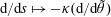 $\text{d}/\text{d}s\mapsto -\unicode[STIX]{x1D705}(\text{d}/\text{d}\tilde{\unicode[STIX]{x1D703}})$
. The equations therefore become
$\text{d}/\text{d}s\mapsto -\unicode[STIX]{x1D705}(\text{d}/\text{d}\tilde{\unicode[STIX]{x1D703}})$
. The equations therefore become
 $$\begin{eqnarray}\displaystyle {\displaystyle \frac{\text{d}}{\text{d}\tilde{\unicode[STIX]{x1D703}}}}U_{p}^{a} & = & \displaystyle -{\displaystyle \frac{1}{\text{i}ak}}((a^{2}k^{2}-\unicode[STIX]{x1D702}_{p}^{2})\unicode[STIX]{x1D733}_{pq}[\tilde{r}]+\unicode[STIX]{x1D733}_{[\,p]q})P_{q}^{a}+\unicode[STIX]{x1D733}_{\{p\}q}U_{q}^{a},\end{eqnarray}$$
 $$\begin{eqnarray}\displaystyle {\displaystyle \frac{\text{d}}{\text{d}\tilde{\unicode[STIX]{x1D703}}}}P_{p}^{a} & = & \displaystyle \text{i}ak\unicode[STIX]{x1D733}_{pq}[\tilde{r}]U_{q}^{a}-\unicode[STIX]{x1D733}_{\{p\}q}P_{q}^{a}.\end{eqnarray}$$
 $V^{a}$
into modal components and eliminating it at the end of the derivation, as doing so produces the equivalent results to eliminating
$V^{a}$
into modal components and eliminating it at the end of the derivation, as doing so produces the equivalent results to eliminating
 $V^{a}$
before we expand about our modal basis.
$V^{a}$
before we expand about our modal basis.


