INTRODUCTION
The most extensive and sustained glaciations in the Quaternary began in the last 900 ka (ca. Marine Isotope Stages [MIS] 24–22 to present) in the Northern Hemisphere and are associated with 100 ka eccentricity-driven glacial–interglacial cycles (Head and Gibbard, Reference Head and Gibbard2015; Hughes and Gibbard, Reference Hughes and Gibbard2018). Despite the obliquity-driven shorter 41 ka glacial–interglacial cycles of the earlier Pleistocene, there is evidence that high- and mid-latitudinal ice sheets in the North Atlantic region have been present since the beginning of the Pleistocene (Thierens et al., Reference Thierens, Pirlet, Colin, Latruwe, Vanhaecke, Lee and Stuut2012). Southern Hemisphere glaciation is an even longer-established phenomenon, with substantial glaciation already a regular occurrence in the Tertiary (Ehlers et al., Reference Ehlers, Gibbard, Hughes, Menzies and van der Meer2018).
In the Italian Dolomites, glaciation became established in MIS 22 (Muttoni et al., Reference Muttoni, Carcano, Garzanti, Ghielmi, Piccin, Pini and Rogledi2003). Comparable evidence is also found north of the Alps in Switzerland and southern Germany (Fiebig et al., Reference Fiebig, Ellwanger, Doppler, Ehlers, Gibbard and Hughes2011). However, the “Deckenschotter” glaciofluvial deposits in Switzerland may represent earlier glaciation, and the older “Höhere Deckenschotter” include vertebrate remains that suggest an age of 2.6–1.8 Ma (Bolliger et al., Reference Bolliger, Feijfar, Graf and Kalin1996). The “Höhere Deckenschotter” are regarded as glaciofluvial deposits. However, no till has been found as yet. In contrast, the “Tiefere Deckenschotter” contain tills. Glaciation during that time might have been more extensive than in the Würmian—see Figure 1 for global chronostratigraphic correlations. The age is uncertain, but the deposits clearly predate the Middle Pleistocene (Preusser et al., Reference Preusser, Graf, Keller, Krayss and Schlüchter2011), which Schlüchter (Reference Schlüchter1989) identified as a major phase of geomorphological change (“Mittelpleistozäne Wende”) in the the Alps. The oldest glaciation identified in the Pyrenees is of late Cromerian age (MIS 16 or 14) (Calvet, Reference Calvet, Ehlers and Gibbard2004). In North America, widespread lowland glaciation (beyond Alaska and the Northern Territories) is first seen during MIS 22 or 20 (Barendregt and Duk-Rodkin, Reference Barendregt, Duk-Rodkin, Ehlers, Gibbard and Hughes2011; Duk-Rodkin and Barendregt, Reference Duk-Rodkin, Barendregt, Ehlers, Gibbard and Hughes2011). In South America, the extensive Great Patagonian glaciation is dated to 1.1 Ma and correlated with MIS 30–34 (Singer et al., Reference Singer, Ackert and Guillou2004).

Figure 1. (color online) Global correlations between terrestrial glacial chronostratigraphic terms and the marine oxygen isotope record. Adapted from the global chronostratigraphic correlation table for the past 2.7 million years by Cohen and Gibbard (Reference Cohen and Gibbard2011).
Following the Early Pleistocene precursors, glaciers reached lowland northern Europe and Siberia in the early Middle Pleistocene shortly before end of the Brunhes–Matuyama palaeomagnetic reversal (~773 ka; Singer et al. Reference Singer, Jicha, Mochizuki and Coe2019), which represents the boundary between the Early and Middle Pleistocene (Head et al., Reference Head, Pillans and Farquhar2008; Head and Gibbard Reference Head and Gibbard2015). These events laid down extensive sheets of glaciogenic deposits across wide areas both on land and beneath the sea. In the northern North Sea, the formation of the Norwegian Channel caused an abrupt change of sedimentary conditions at about this time (Ottesen et al., Reference Ottesen, Dowdeswell and Bugge2014). While 100 ka cycles began ca. MIS 24–22 (Elderfield et al., Reference Elderfield, Ferretti, Greaves, Crowhurst, McCave, Hodell and Piotrowski2012), the largest-amplitude 100 ka glaciations started with MIS 16, which marked the completion of the Early–Middle Pleistocene transition (Head and Gibbard, Reference Head and Gibbard2005; Mudelsee and Schulz, Reference Mudelsee and Schulz1997; Hughes and Gibbard, Reference Hughes and Gibbard2018).
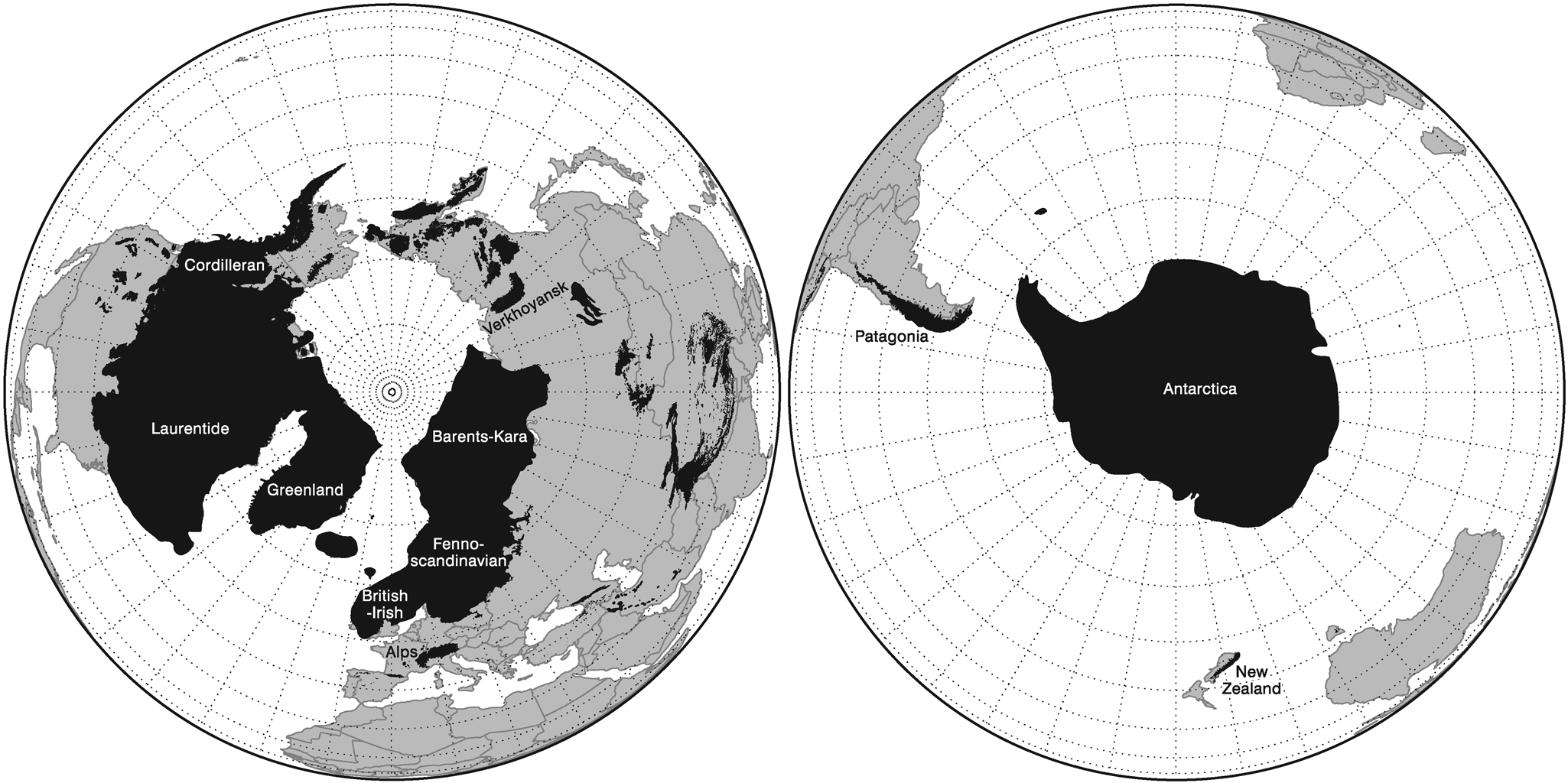
Subsequently, major ice sheets repeatedly extended over large regions of North America during the Middle Pleistocene pre-Illinoian events MIS 16, 12, and 6 (Illinoian s.s.) and the Late Pleistocene MIS 5d–2 (Wisconsinan). The Laurentide Ice Sheet formed over large areas of Canada, reaching as far south as 38°N in the United States during the Late Pleistocene (Dyke and Prest, Reference Dyke and Prest1987; Fig. 2). More significantly, the change in ice volume between glacial–interglacial cycles was the largest single contribution to the global sea-level changes. This was 70–90 m for the last glacial–interglacial cycle (Stokes et al., Reference Stokes, Tarasov and Dyke2012), which represents well over half the global ice contribution to glacial–interglacial sea-level change. Today, the largest ice sheet is restricted to Greenland, with much smaller ice caps present in Canada.

Figure 2. Maximum extent of glaciation around the globe during the last glacial–interglacial cycle (Weichselian, Wisconsinan, and Valdaian Stages and equivalents). The extents depicted here are diachronous with ice masses reaching their maximum positions at different times. The extents would have also varied in different glacial–interglacial cycles, although the general differences in extents of the largest continental ice masses is typical of the relative contributions of ice on Earth by the major regional ice masses. This figure illustrates the relative sizes of the ice masses and their spatial distributions and highlights the spatial dominance of the ice masses in the Northern Hemisphere. Redrawn and adapted from Ehlers and Gibbard (Reference Ehlers and Gibbard2007) and Hughes et al. (Reference Hughes, Gibbard and Ehlers2013).
The marine oxygen isotope record provides the main basis for defining Quaternary glacial–interglacial cycles (Lisiecki and Raymo, Reference Lisiecki and Raymo2005) and has long been considered to represent a record of global ice volume (Shackleton, Reference Shackleton1967). The marine isotope record is widely used as the global reference for subdividing the Quaternary, and the scheme of stages and substages in the marine isotope record continues to underpin the Quaternary time scale (Lisiecki and Raymo, Reference Lisiecki and Raymo2005; Railsback et al., Reference Railsback, Gibbard, Head, Voarintsoa and Toucanne2015; Fig. 1). The marine isotope record has the advantage of being derived from quasi-continuous sedimentary sequences on the deep-ocean floors, whereas the glacial records on land are inherently fragmentary. However, the marine isotope record is a composite signal of fluctuations in global ice volume and does not provide information on the spatial pattern of glaciations. Furthermore, because changes in global ice volume are dominated by the Laurentide Ice Sheet (Fig. 2), it is not necessarily representative of the pattern and scale of glaciations in other parts of the world. This poses problems for direct terrestrial–marine correlation (Gibbard and West, Reference Gibbard and West2000), and care must be taken to isolate glacial records using single proxies such as the marine isotope record. This is also true for other indirect proxies for global glaciations, some of which are used here, such as sea-level and ice-core records. Thus, a collective approach is necessary to decipher the patterns of global glaciations, especially where terrestrial glacial records are absent, ambiguous, or poorly dated, which is often the case, especially for the Middle Pleistocene glaciations.
The application of numerical dating of Late Pleistocene glaciations is increasingly demonstrating the asynchronies in the timing of glacial maxima on a global scale (Hughes et al., Reference Hughes, Gibbard and Ehlers2013). While the differing timing of mountain glaciations compared with the continental ice sheets has been known for decades (e.g., Gillespie and Molnar, Reference Gillespie and Molnar1995), there is now also evidence that the timing of maximum extents of major ice sheet margins may have differed by as much as tens of thousands of years. Such differences appear to result from the contrasting regional geographical situations, where differing ocean and atmospheric circulatory patterns influence precipitation and air temperatures (Hughes et al., Reference Hughes, Gibbard and Ehlers2013).
Differences in the pattern and timing of glacial extent are also notable between different glacial–interglacial cycles (cf. Margari et al., Reference Margari, Skinner, Tzedakis, Ganopolski, Vautravers and Shackleton2010, Reference Margari, Skinner, Hodell, Martrat, Toucanne, Grimalt, Gibbard, Lunkka and Tzedakis2014; Hughes and Gibbard, Reference Hughes and Gibbard2018; Batchelor et al., Reference Batchelor, Margold, Krapp, Murton, Dalton, Gibbard, Stokes, Murton and Manica2019). The largest glaciations of the last 800 ka, such as in MIS 5d-2, were characterized by an early advance of glaciers followed by an interlude, then a second major advance leading to the global glacial maxima within the glacial–interglacial cycles (Hughes and Gibbard, Reference Hughes and Gibbard2018). This corresponds to the classic asymmetrical pattern of ice buildup in 100 ka glacial–interglacial cycles (Broecker and van Donk, Reference Broecker and van Donk1970). The greater magnitude of the second major global ice advance is reflected in the larger dust peak associated with it compared with the first major advance, such as when comparing MIS 4 and 2 in the last glacial–interglacial cycle (Fig. 3). However, Hughes and Gibbard (Reference Hughes and Gibbard2018) identified differences between glacial–interglacial cycles, with some exhibiting different patterns. For example, in MIS 10 and 8, the first phase of glacial buildup corresponded to the largest dust peaks, and the later global glacial maxima was associated with much smaller dust peaks in Antarctic ice-core records (Fig. 4). Other anomalies are also evident when considering the pattern of glaciations from the perspective of the marine isotope record. For example, some major stadials occur within interglacial complexes (such as MIS 7d) (Ruddiman and McIntyre, Reference Ruddiman and McIntyre1982). These represent “missing glaciations” in the sense that they are rarely recorded on land. However, it is important to understand that glaciers would have been more extensive than today in most areas of the world in all cold intervals of major glacial–interglacial cycles. The evidence that glaciations are “missing” simply arises because their spatial coverage has been overridden by later, more extensive glaciations.

Figure 3. The dust records from Greenland (NGRIP) and Antarctica (EPICA) ice cores for the last glaciation in MIS 5d-2. The top diagram shows the dust concentration (Ruth et al., Reference Ruth, Bigler, Rothlisberger, Siggaard-Andersen, Kipfstuhl, Goto- Azuma, Hansson, Johnsen, Lu and Steffensen2007) record from the NGRIP core (on the GICC05 age model). The bottom diagram shows dust flux (Lambert et al., Reference Lambert, Bigler, Steffensen, Hutterli and Fischer2012) from EPICA, Antarctica (on the EDC3 age model). The grey shaded bars represent the cold intervals (from left to right) of MIS 2, 4, 5b and 5d. The records show a strong correlation in dust records between Greenland and Antarctica, and this supports the assertion that dust records in either polar hemisphere reflect the state of the global hydrological cycle and the global atmosphere. This observation provides the template for interpreting earlier glaciations, with drier and dustier atmosphere directly related to increasing global ice coverage. This interhemispheric comparability is important, because beyond the last interglacial, studies must currently rely on the Antarctic ice-core records. Adapted from Hughes and Gibbard (Reference Hughes and Gibbard2015).
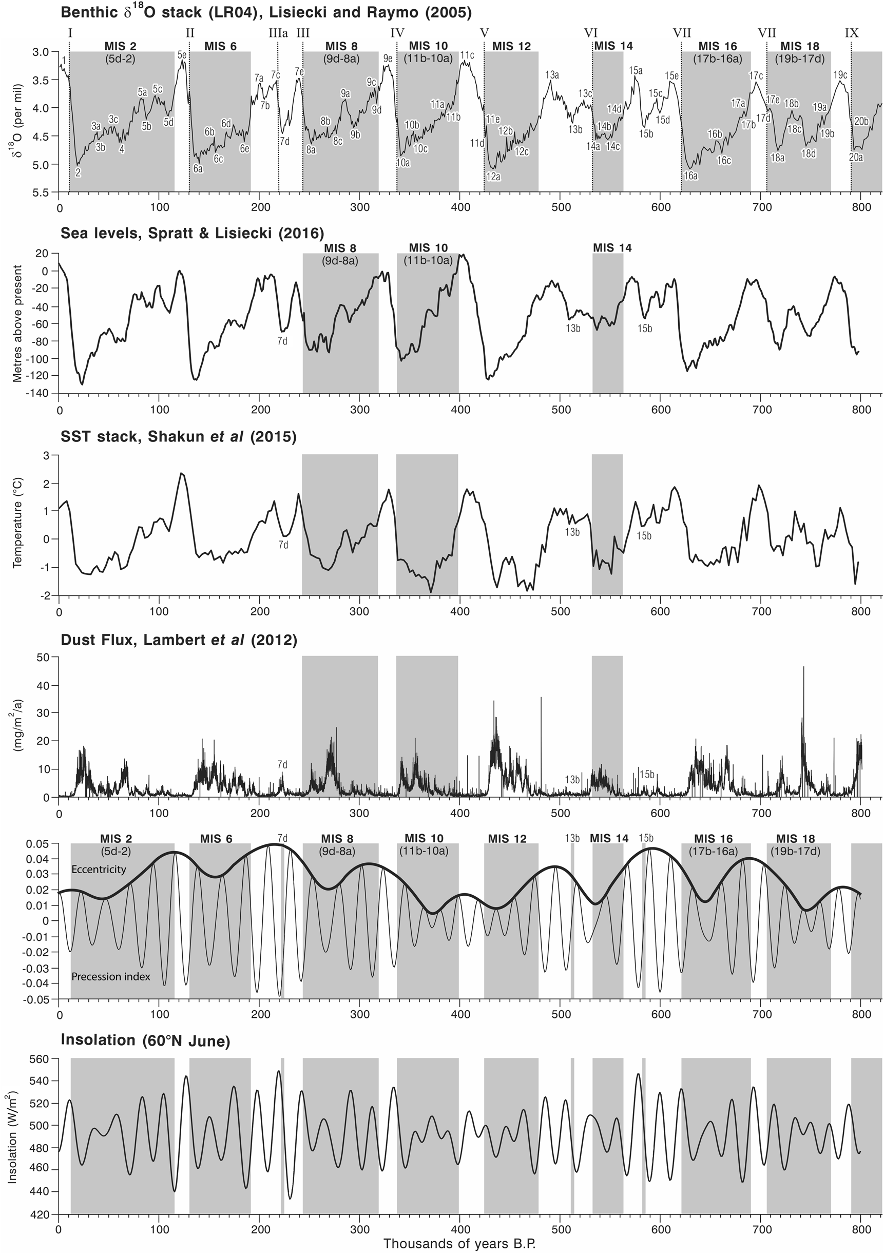
Figure 4. Graphs showing link between the structure of glacial–interglacial cycles indicated in the global benthic stack of Lisiecki and Raymo (Reference Lisiecki and Raymo2005), global sea levels extracted from a global stack of sea-level records (from Spratt and Lisiecki, Reference Spratt and Lisiecki2016), global sea-surface temperatures (SSTs) from 49 paired SST-planktonic δ18O records (Shakun et al., Reference Shakun, Lea, Lisiecki and Raymo2015), and dust flux from the EPICA Dome C ice-core record (Lambert et al., Reference Lambert, Bigler, Steffensen, Hutterli and Fischer2012). The Roman numerals (I, II, III, IV, etc.) over the global benthic stack indicate the positions of the respective glacial terminations. The lower two graphs illustrate solar parameters for the last 800 ka. The second from bottom graph shows the precession index and the eccentricity index from Berger and Loutre (Reference Berger and Loutre1991) and Berger (Reference Berger1992). The precession index (climatological precession parameter: e sin ω; values from −1 to + 1) is an indicator of the amplitude of the seasonal cycle with a move towards autumn/winter perihelion at peaks and towards an earlier spring/summer perihelion at troughs and is determined by the variations in eccentricity (dimensionless value between 0 and 1). The bottom graph shows June insolation data at 60°N (Berger and Loutre, Reference Berger and Loutre1991; Berger, Reference Berger1992).
We test the hypothesis that the cold phases of some glacial–interglacial cycles were characterized by less extensive glaciations than others. To do this, we examine in this article the evidence for Middle Pleistocene glaciations after MIS 16, which marked the onset of the largest 100 ka glacial cycles (Hughes and Gibbard, Reference Hughes and Gibbard2018). We focus on MIS 8, 10, and 14 together with other intermediate intervals (MIS 7d, 13b, and 15b) and test whether the concept of “missing glaciations” is valid for these cold intervals. We aim to explore reasons for the differences in the terrestrial glacial records between and within glacial–interglacial cycles by examining the wider environmental imprint of global glaciations alongside the drivers of global climate change.
METHODOLOGICAL APPROACH
Glacial records
The geologic and geomorphological evidence for glaciation is based on published papers from sites around the world. This evidence includes large compilations and reviews such as those in Ehlers et al. (Reference Ehlers, Gibbard and Hughes2011a, Reference Ehlers, Gibbard, Hughes, Ehlers, Gibbard and Hughes2011b) and many other sources, including many new data sets from the last few years. A key focus is on dated records, which for the Middle Pleistocene glacial record are dominated by cosmogenic exposure, optically stimulated luminescence (OSL), and uranium-series dating.
Indirect records of glaciation and global climate
Marine isotope records
Marine oxygen isotope records provide the classic proxy for global ice volume (Shackleton, Reference Shackleton1967) and underpin modelling approaches for ice sheet reconstructions through time where direct evidence of glaciation is not available (e.g., Batchelor et al., Reference Batchelor, Margold, Krapp, Murton, Dalton, Gibbard, Stokes, Murton and Manica2019). The driver of cyclic fluctuations in marine oxygen isotopes from foraminiferal tests has long been attributed to orbital forcing (Hays et al., Reference Hays, Imbrie and Shackleton1976), and this provides the time frame to which the marine isotope record is tuned (Imbrie et al., Reference Imbrie, Hays, Martinson, McIntyre, Mix, Morley, Pisias, Prell, Shackleton, Berger, Imbrie, Hays, Kukla and Saltzman1984; Ruddiman et al., Reference Ruddiman, Raymo, Martinson, Clement and Backman1989; Lisiecki and Raymo, Reference Lisiecki and Raymo2005; Fig. 4). However, the marine oxygen isotope record is not a pure record of global ice volume but is a record of both global ice volume and deep-ocean temperature (Spratt and Lisiecki, Reference Spratt and Lisiecki2016). Furthermore, as noted earlier, changes in the Laurentide Ice Sheet through glacial–interglacial cycles dominate the global ice volume component of the marine isotope signal due to its large size relative to other ice masses on Earth (Fig. 2). Consequently, the marine isotope record is not representative of the spatial complexity of global glaciations (Hughes et al., Reference Hughes, Gibbard and Ehlers2013).
Sea-level records
Global ice volume is closely intertwined with global sea levels, and the magnitude of glaciations is reflected in sea-level changes. Global sea levels through the last 800 ka were assessed using the data of Spratt and Lisiecki (Reference Spratt and Lisiecki2016) (Fig. 4). In their paper, Spratt and Lisiecki (Reference Spratt and Lisiecki2016) analysed seven Late Pleistocene sea-level records for the interval 0–430 ka and five for the interval 0–798 ka that have converted the oxygen isotope content of the calcite tests of foraminifera (δ18Oc) to sea level. The seven records included an inverse ice volume model (Bintanja et al., Reference Bintanja, Roderik and van de Wal2005), Pacific benthic δ18O of seawater (δ18Osw) (Elderfield et al., Reference Elderfield, Ferretti, Greaves, Crowhurst, McCave, Hodell and Piotrowski2012), a global stack of planktonic δ18Osw (Shakun et al., Reference Shakun, Lea, Lisiecki and Raymo2015), relative sea level from the Mediterranean (Rohling et al., Reference Rohling, Grant, Bolshaw, Roberts, Siddall, Hemleben and Kucera2014), Atlantic benthic δ18Osw (Sosdian and Rosenthal, Reference Sosdian and Rosenthal2009), δ18Oc regression (Waelbroeck et al., Reference Waelbroeck, Labeyrie, Michel, Duplessy, McManus, Lambeck, Balbon and Labracherie2002), and a relative sea level from the Red Sea (Rohling et al., Reference Rohling, Grant, Bolshaw, Roberts, Siddall, Hemleben and Kucera2009). The longer record (used in this paper) for the interval 0–798 ka excluded the δ18Oc regression (Waelbroeck et al., Reference Waelbroeck, Labeyrie, Michel, Duplessy, McManus, Lambeck, Balbon and Labracherie2002) and the relative sea level from the Red Sea (Rohling et al., Reference Rohling, Grant, Bolshaw, Roberts, Siddall, Hemleben and Kucera2009) (see Spratt and Lisiecki, Reference Spratt and Lisiecki2016, Table 1).
Table 1. Sea-level estimates from the global stack of Spratt and Lisiecki (Reference Spratt and Lisiecki2016) in order of magnitude. These values are obtained from the long stack (0–798 ka) of five sea-level reconstructions. The marine isotope stages listed represent cold-climate intervals within glacial–interglacial cycles.

a MIS 15b, 13b, and 7d are stadials within interglacials.
Hughes and Gibbard (Reference Hughes and Gibbard2018) analysed sea-level changes through glacial–interglacial cycles using the data of Shakun et al. (Reference Shakun, Lea, Lisiecki and Raymo2015), who used planktonic δ18Osw to correct the δ18O stack for non–ice volume effects. However, in their analysis of global sea-level change through glacial–interglacial cycles, Spratt and Lisiecki (Reference Spratt and Lisiecki2016) noted that because the surface ocean is affected by greater hydrological variability and characterises a smaller ocean volume than the deep ocean, planktonic δ18Osw may differ more from ice volume changes than benthic data.
Sea-surface temperature records
Shakun et al. (Reference Shakun, Lea, Lisiecki and Raymo2015) exploited the temperature component of planktonic δ18O records from 49 cores around the globe to calculate a stacked record of global sea-surface temperatures (SSTs) (Fig. 4). This now enables insights into global shifts in both climate and ice volume during glacial–interglacial cycles. This is significant, because it avoids the Laurentide problem, wherein global ice volumes are dominated by a single regional ice mass. While ice sheets do affect SSTs at the regional scale, global SSTs between different oceans are much less likely to be dominated by regional ice dynamics.
While the surface ocean is undoubtedly subject to greater hydrological variability (see Spratt and Lisiecki, Reference Spratt and Lisiecki2016) and surface atmospheric processes, this is useful for gauging the state of the Earth's ocean–atmosphere interface. At individual scales, SST records are likely to be quite variable, but when combined, the stack of 49 cores used by Shakun et al. (Reference Shakun, Lea, Lisiecki and Raymo2015) from sites located at 0–60°N and 0–60°S in the Pacific, Atlantic, and Indian Oceans does provide a global summary of the state of the ocean–atmosphere interface through glacial–interglacial cycles.
Ice-core records
Dust content in polar ice cores can provide insights into the state of the global atmosphere through time, and this was used by Lambert et al. (Reference Lambert, Delmonte, Petit, Bigler, Kaufmann, Hutterli, Stockler, Ruth, Steffensen and Maggi2008, Reference Lambert, Bigler, Steffensen, Hutterli and Fischer2012) to assess dust flux over Antarctica during multiple glacial–interglacial cycles. Hughes and Gibbard (Reference Hughes and Gibbard2015; Reference Hughes and Gibbard2018) argued that peaks in Antarctic dust in glacial–interglacial cycles corresponded to global ice buildup in both hemispheres, and this was used as an indirect indicator of global glacial behaviour in glacial–interglacial cycles. This argument was largely built on observations from the last glacial–interglacial cycle, in which large ice buildup in MIS 4 and 2, for example, was associated with peaks in dust not only in Greenland but also in Antarctica (Hughes and Gibbard, Reference Hughes and Gibbard2015; Fig. 3).
Given that the Greenland ice-core records only span from the last interglacial, Antarctic records must be relied upon for earlier glacial–interglacial cycles. Dust flux over Antarctica has a close correlation with temperature as climate becomes colder (Lambert et al., Reference Lambert, Delmonte, Petit, Bigler, Kaufmann, Hutterli, Stockler, Ruth, Steffensen and Maggi2008). Comparison of Antarctic ice-core dust records with loess/palaeosol sequences from the Chinese Loess Plateau (Kukla et al., Reference Kukla, An, Melice, Gavin and Xiao1994) confirms the synchroneity of global changes in atmospheric dust load (Lambert et al., Reference Lambert, Delmonte, Petit, Bigler, Kaufmann, Hutterli, Stockler, Ruth, Steffensen and Maggi2008). However, being a Southern Hemisphere record, comparisons of dust peak magnitudes cannot necessarily be transferred to interpreting the size of global ice volume, only the temporal pattern and possibly the hemispheric distribution of ice masses. Nevertheless, Antarctic dust records are broadly representative of the global hydrological cycle, with increasing dust indicating a cooler and drier global atmosphere that is directly associated with the extent of global glaciations.
Dust records may be a better reflection of global ice spatial coverage on land than marine isotope records, which partially reflect ice volume. This is because increased ice coverage over land surfaces causes increased aridity in peripheral areas due to the effects of ice masses on regional climate (Manabe and Broccoli, Reference Manabe and Broccoli1985). This occurs today where strong anticyclones form over modern ice sheets (Hobbs, Reference Hobbs1945). The aridity effects would have been compounded during the Pleistocene cold phases due to the effects of not just low precipitation but also low atmospheric CO2 on plant growth (Claquin et al., Reference Claquin, Roelandt, Kohfeld, Harrison, Tegen, Prentice and Balkanski2003).
Drivers of global glaciations: solar forcing and CO2
We examine the patterns of Earth-orbital changes and glacial–interglacial cycles to see whether there is any relationship between “missing glaciations” and orbital forcing. Solar radiation is important when considering glaciations, because it controls the energy receipt to the Earth and thereby impacts glacial mass balance, especially ablation. In their synthesis of the last 10 glacial–interglacial cycles, Hughes and Gibbard (Reference Hughes and Gibbard2018) showed that variations in solar radiation in the Northern Hemisphere were responsible for ~50%–60% of variations in global ice volume. For example, troughs in solar radiation at the end of interglacials and beginning of subsequent cold stages are thought to be associated with rapid glacial advances in the continental interiors and high- and mid-latitude mountains (Hughes and Gibbard, Reference Hughes and Gibbard2018). This hypothesis is tested further here by quantifying the magnitude of solar peak–trough changes at the transition between interglacial and glacial intervals (Fig. 4). This was done by calculating a value for solar-trough magnitude (STM), which describes the trough magnitude and time span at 60°N. This is derived by taking the median (50th percentile) solar radiation value (W/m2) between the trough and the preceding peak (s m) and dividing this by the trough time span (s t) (defined by the time in years between the trough and the preceding peak), then inverting this value:
STM = 1/(s m/s t)
We also examine the orbital record further by isolating the effects of orbital parameters such as eccentricity, obliquity, and precession on global glacial dynamics within and between glacial–interglacial cycles. Eccentricity controls the shape of the Earth's orbit around the sun and directly affects the influence of variations of precession (i.e., on the timing of perihelion and aphelion) and the seasonal distribution of solar radiation. The interaction of eccentricity with precession is indicated in the precession index (Fig. 4). In addition to solar radiation, Ganopolski et al. (Reference Ganopolski, Winkelmann, Schellnhuber, Ehlers, Gibbard and Hughes2016) highlighted the importance of CO2 in glacial inception. They identified points in time when low CO2 corresponded with low insolation as potential triggers for global ice buildup. This hypothesis implies that low insolation alone cannot explain global glacial inception. Instead, it is the combination of insolation forcing with atmospheric CO2 concentrations that drives glacial inceptions. Over the longer term, declining atmospheric CO2 through the Quaternary has been linked to the removal of weathered regolith by glacial erosion over North America and Europe (Clark and Pollard, Reference Clark and Pollard1998). This causal mechanism may partly explain the transition to the large-magnitude 100 ka glacial–interglacial cycles at the Early–Middle Pleistocene transition (Clark and Pollard, Reference Clark and Pollard1998; Ganopolski and Calov, Reference Ganopolski and Calov2011; Tabor and Poulsen, Reference Tabor and Poulsen2016; Willeit et al., Reference Willeit, Ganopolski, Calov and Brovkin2019).
Terminology
There are three ways to define glacial–interglacial cycles (Hughes and Gibbard, Reference Hughes and Gibbard2018):
1. the periods between glacial terminations;
2. the periods of cold phases defined by global SSTs within glacial–interglacial cycles (cf. Shakun et al., Reference Shakun, Lea, Lisiecki and Raymo2015), and;
3. the span of traditional subdivision of cold intervals based on marine isotope stages and substages (Railsback et al., Reference Railsback, Gibbard, Head, Voarintsoa and Toucanne2015).
The term cold stage refers to climatostratigraphic/chronostratigraphic units such as the Weichselian or Wisconsinan in Europe or North America, respectively, which are equivalent to MIS 5d-2. This is complicated by the fact that some cold stages in this definition span multiple glacial–interglacial cycles, such as the Saalian and Wolstonian Stages in continental Europe and the British Isles, respectively. Marine oxygen isotope stages are distinct from chronostratigraphic cold stages and sometimes multiple marine isotope stages make up a single cold stage in the strict sense. For example, the Weichselian/Wisconsinan stages include MIS 5d-2 and also the early part of MIS 1. A global correlation table based on the chart of Cohen and Gibbard (Reference Cohen and Gibbard2011) is provided in Figure 1 to aid cross-comparison between marine isotope events and terrestrial chronostratigraphy.
THE “MISSING GLACIATIONS”
MIS 8 (Middle Saalian and equivalents)
MIS 8 occurs within a larger glacial–interglacial cycle between termination IV and III (Fig. 4). Overall, this was a relatively weak glacial–interglacial cycle. The glacial inception occurred at the boundary of MIS 9d/e at ca. 320 ka. MIS 8 has a weak signal of global glaciation in many records, particularly benthic δ18O (Lang and Wolff, Reference Lang and Wolff2011), and is second only to MIS 14 in terms of maximum δ18O values for the last 10 glacial–interglacial cycles (Fig. 4). At −93.27 m, MIS 8 had the highest sea levels of the last six 100 ka glaciations (Table 1). The lowest sea levels do not coincide with the trough in benthic δ18O values (at 252 ka) but occurred ca. 18 ka earlier at 270 ka in MIS 8c (Fig. 4). A strong interstadial (MIS 9a) separates two marine isotope troughs (MIS 8a-c and 9b).
The solar-trough magnitude at the beginning of this glacial–interglacial cycle was one of the weakest of the last seven glacial–interglacial cycles (Table 2). This is likely to have resulted in a weak glacial inception and explains the weak stadial conditions in MIS 9d, which is characterised by relatively minor excursions in benthic and planktonic isotope values and moderate influence of subpolar water masses (Roucoux et al., Reference Roucoux, Tzedakis, de Abreu and Shackleton2006). In their core from the Iberian margin, Roucoux et al. (Reference Roucoux, Tzedakis, de Abreu and Shackleton2006) argued that the pollen evidence suggests a less arid and cold climate than during other stadial intervals, when steppe was more abundant and temperatures offshore were lower.
Table 2. Solar radiation peak-trough amplitude at 60°N early in cold stages or at the end of preceding interglacials. Solar-trough magnitude describes the peak-trough magnitude and time span. This is derived by taking the median value between the preceding solar peak and subsequent trough and scaling (dividing) this by the peak to trough time span, then inverting this calculated value. Solar radiation data are derived from Berger and Loutre (Reference Berger and Loutre1991) and Berger (Reference Berger1992). Marine Isotope Stages are listed in descending order of solar-trough magnitude. The Marine Isotope Stages associated with the “Missing Glaciations” are shown separately at the bottom of the table.

a Insolation (W/m2).
Dust flux over Antarctica for MIS 8 reached some of the highest and sustained levels of the last million years, reaching values comparable with MIS 6, yet more sustained, and greater than MIS 5d-2 (Fig. 4). Significantly, the dust peak in Antarctica does not coincide with the largest marine isotope trough of MIS 8a. Instead, it occurs earlier at ca. 272 ka in MIS 8c, coinciding with the lowest sea levels. Hughes and Gibbard (Reference Hughes and Gibbard2018) noted that the first dust peak also coincides with the lowest CO2 levels (Ganopolski et al., Reference Ganopolski, Winkelmann, Schellnhuber, Ehlers, Gibbard and Hughes2016) and the coldest global SSTs of this glacial period (Shakun et al., Reference Shakun, Lea, Lisiecki and Raymo2015). Pollen records from a marine core on the Iberian margin match these patterns and show the most extreme glacial conditions of MIS 8 occurred during the early part, followed by an interval of warmer conditions and tree population expansion after 263 ka (Roucoux et al., Reference Roucoux, Tzedakis, de Abreu and Shackleton2006). This suggests that the configuration of controls of global climate (including insolation, atmospheric composition, land cover, sea ice, and the ice sheets themselves) were different in MIS 8 from other glaciations, such as MIS 6 and 5d-2. In these later glaciations, the global ice maxima and associated cold and dry indicators occurred towards the end of the glacial–interglacial cycle.
Examination of the record of glaciation during this period (i.e., ca. 320–243 ka) repeatedly shows that evidence of glaciation is poorly represented throughout much of the world's glaciated regions. In northern Europe, the traces of glaciation that can be reliably attributed to this time are rare. The few deposits that have been identified in northwest Europe are mainly based on isolated numerical age determinations, especially OSL or amino acid racemisation analyses of adjacent sediments or their contained fossil materials. For example, the most often quoted example is that reported by Beets et al. (Reference Beets, Meijer, Beets, Cleveringa, Laban and van der Spek2005) suggesting that pre-Late Saalian (i.e., Middle Saalian; MIS 8) till occurs in the North Sea basin based on geophysical, micropalaeontological, and amino acid age evidence. While there is no question that till occurs at the site, there remains scepticism about the age attribution among Dutch workers who generally attribute these deposits to the Late Saalian (MIS 6; Cohen, K.M., personal communication, 2017). Despite other possible MIS 8 records from other circum–North Sea localities (e.g., White et al., Reference White, Bridgland, Howard, Westaway and White2010, Reference White, Bridgland, Westaway and Straw2017; Davies et al., Reference Davies, Roberts, Bridgland, Ó Cofaigh, Riding, Demarchi, Penkman and Pawley2012; Bridgland et al., Reference Bridgland, Howard, White and White2014; Roskosch et al., Reference Roskosch, Winsemann, Polom, Brandes, Tsukamoto, Weitkamp, Bartholomäus, Henningsen and Frechen2015) all of these remain equally equivocal. In contrast, as in the Netherlands, recent dating evidence from eastern England has confirmed that a major glaciation did occur in MIS 6 (Evans et al., Reference Evans, Roberts, Bateman, Ely, Medialdea, Burke, Chiverrell, Clark and Fabel2019) confirming the Wolstonian (= Saalian) age of a glaciation that reached into the Fenland basin in eastern England (Gibbard et al., Reference Gibbard, West and Hughes2018). The lack of a regional till sheet and consistent biostratigraphy appears to support the view that glacial ice did not extend into the central western European area and the central and southern North Sea basin (Huuse, M. personal communication, 2017) during MIS 8. However, there is evidence for Middle Saalian glaciation that reached the continental shelf edge off Norway, Svalbard, and Scotland, according to Sejrup et al. (Reference Sejrup, Larsen, Landvik, King, Haflidason and Nesje2000, Reference Sejrup, Hjelstuen, Dahlgren, Haflidason, Kuijpers, Nygård, Praeg, Stoker and Vorren2005). In southern Jæren in southwestern Norway, this glaciation is represented by the Vigrestad Till (glacial F: Sejrup et al., Reference Sejrup, Larsen, Landvik, King, Haflidason and Nesje2000). In Denmark, westward-flowing meltwater streams deposited sand and gravels over much of central and southern Jylland. These streams derive from the first Saalian ice advance that occurred during MIS 8, which deposited the Treldenæs Till (Houmark-Nielsen, Reference Houmark-Nielsen, Ehlers and Gibbard2004, Reference Houmark-Nielsen, Ehlers, Gibbard and Hughes2011). This Norwegian Saale advance invaded Denmark from the north, probably terminating south of the Danish–German border in Schleswig-Holstein (Houmark-Nielsen, Reference Houmark-Nielsen, Ehlers, Gibbard and Hughes2011).
In northwest Europe, Toucanne et al. (Reference Toucanne, Zaragosi, Bourillet, Cremer, Eynaud, Van Vliet-Lanoe and Penaud2009a) noted that Fleuve Manche fluvial discharge through the English Channel was significantly less during MIS 8 than during MIS 6 and 2 (indicated by lower mass accumulation rates [MAR] in Fig. 5). This is consistent with smaller ice masses in northern Europe and the Alps, the meltwater from which drained into this river system in MIS 8. Furthermore, in the northeast Atlantic Ocean at Ocean Drilling Programme (ODP) Site 980 (55°29′N, 14°42′W) summer SSTs were generally warmer in MIS 8 than in MIS 6 and 2 (McManus et al., Reference McManus, Oppo and Cullen1999). However, oscillations in SSTs were large, with minimum temperatures on a par with MIS 6 and 2. In fact, the quantities of ice-rafted debris (IRD) in the northeast Atlantic during MIS 8 and 10 were significantly larger than in MIS 6 and 2 (McManus et al., Reference McManus, Oppo and Cullen1999). This was related to high-amplitude millennial-scale climate change, which is also reflected in terrestrial vegetation records in Europe (Fletcher et al., Reference Fletcher, Müller, Koutsodendris, Christanis and Pross2013). The muted signal in the Fleuve Manche discharge in contrast to a strong signal in the IRD in the northeast Atlantic suggests the configuration of ice masses in this region differed between glacial–interglacial cycles.

Figure 5. (color online) Top, mass accumulation rates (MAR) in marine sediment records in the Bay of Biscay, northeast Atlantic Ocean (from Toucanne et al., Reference Toucanne, Zaragosi, Bourillet, Cremer, Eynaud, Van Vliet-Lanoe and Penaud2009a). The MAR graph is from sites MD03-2692 (46°49.72′N, 9°30.97′W), MD01-2448, and MD04-2818. Lower MAR in MIS 10 and 8 compared with MIS 5d-2 and 6 are interpreted as indicating less glaciofluvial discharge, primarily through the former English Channel fluvial system (Fleuve Manche). The XRF Ti-Ca ratio reflects terrigenous sediment input, but is also associated with an ice-rafted debris (IRD) source. The IRD graph is from site ODP 980 from farther north in the northeast Atlantic Ocean (55°29′N, 14°42′W) off the British–Irish continental shelf (data from McManus et al., Reference McManus, Oppo and Cullen1999). The bottom map shows the locations of these core sites relative to the former ice masses. The approximate positions of the Late Pleistocene ice limits for the northern ice sheets (BIIS, British–Irish Ice Sheet; FIS, Fennoscandian Ice Sheet) are given for reference in white shading together with the Late Saalian (MIS 6) ice limits shown in red/grey (Drenthe advance) and black (Warthe advance). The outlines and positions of ice masses in central and southern Europe are schematic due to scale. The white arrows and the associated lowercase letters identify the main European rivers: a, Fleuve Manche; b, Solent; c, Thames; d, Meuse; e, Rhine; f, Ems; g, Wesser; h, Elbe; i, Seine; j, Loire; k, Gironde; l, Pô. Redrawn and adapted from Toucanne et al. (Reference Toucanne, Zaragosi, Bourillet, Cremer, Eynaud, Van Vliet-Lanoe and Penaud2009a). (For interpretation of the references to color in this figure legend, the reader is referred to the web version of this article.)
In Poland, the Krznanian glaciations are correlated with MIS 8 (Lindner and Marks, Reference Lindner and Marks1999). According to Marks (Reference Marks, Ehlers, Gibbard and Hughes2011), Poland was invaded by ice sheets derived from Scandinavia during the Liwiecian, Krznanian, and Odranian intervals within the Saalian Stage. The limit of the Odranian glaciation can be mapped at the modern land surface, whereas the Liwiecian and Krznanian are buried by younger deposits. During the latter, an ice sheet advanced into eastern Poland, reaching as far south as the northern foreland of the South Polish Uplands, and it probably also approached the Silesian Upland. This advance may have also crossed the Baltic states, Latvia and Lithuania, and presumably parts of Belarus.
In neighbouring European Russia, glaciation during this period seems to have been markedly less extensive than during the Late Saalian–equivalent Dniepr and Moscow glaciations (MIS 6) (Velichko et al., Reference Velichko, Faustova, Pisareva, Gribchenko, Sudakova, Lavrentiev, Ehlers, Gibbard and Hughes2011; Fig. 1). However, east of the Urals it is represented by the substantial till of the Samarovo glaciation, the deposits of which form the maximum glacial drift boundary in western Siberia. This major glaciation is correlated with MIS 8 (Fig. 6) based on regional stratigraphic successions (Astakhov et al., Reference Astakhov, Shkatova, Zastrozhnov and Chuyko2016).

Figure 6. (color online) Limits of the Eurasian contiguous ice sheets during the Middle and Late Pleistocene. Adapted from information in Svendsen et al. (Reference Svendsen, Alexanderson, Astakhov, Demidov, Dowdeswell, Funder and Gataullin2004), Astakhov et al. (Reference Astakhov, Shkatova, Zastrozhnov and Chuyko2016) and Hughes and Gibbard (Reference Hughes and Gibbard2018). East of the Urals, the most extensive glaciation occurred in MIS 8, although evidence of this glaciation is largely absent to the west in Europe.
While the limit is based on boreholes and rare natural sections in the west Siberian Plain, in the central Siberian Uplands the boundary has been mapped based on chains of push moraines and occasionally where it overlies interglacial fluvial deposits in buried valleys (Rudenko et al., Reference Rudenko, Fainer and Fainer1984; Astakhov, Reference Astakhov, Ehlers, Gibbard and Hughes2011). In the western Siberian Plain and the central Siberian Plateau, the Samarovo glaciation was consistently much more extensive than the later Taz glaciation, which is thought to date from later in the Saalian Stage in MIS 6 (Astakhov et al., Reference Astakhov, Shkatova, Zastrozhnov and Chuyko2016). Given the scale of the land areas involved, these Siberian ice masses would have been major contributors to global ice volume.
In the mountains of central and southern Europe, evidence of glaciation in MIS 8 has been recognised in Iberia (Fernández Mosquera et al., Reference Fernández Mosquera, Marti, Vidal Romaní and Weigel2000; Vidal Romaní et al., Reference Vidal Romaní, Mosquera and Marti2015), Italy (Giraudi and Giaccio, Reference Giraudi and Giaccio2017), and the Alps (Preusser et al., Reference Preusser, Graf, Keller, Krayss and Schlüchter2011). In Baden-Württemberg and Bavaria, southern Germany, the multiphased Riss glaciation is provisionally correlated with MIS 10–6 (Doppler et al., Reference Doppler, Kroemer, Rögner, Wallner, Jerz and Grottenthaler2011). In the Balkans, there is also some evidence of MIS 8 glaciation (Hughes et al., Reference Hughes, Woodward, van Calsteren and Thomas2011). In the Italian Apennines, Giraudi et al. (Reference Giraudi, Bodrato, Ricci Lucchi, Cipriani, Villa, Giaccio and Zuppi2011) reported that there was no evidence for glaciation in MIS 8, unlike for other Middle Pleistocene glaciations. However, later work in the same basin revealed evidence of two glaciations between 350 and 130 ka, and these were correlated with MIS 8 and 6, although the relative sizes of these two glaciations was not established (Giraudi and Giaccio, Reference Giraudi and Giaccio2017).
In North America, evidence of glaciation attributed to the MIS 8 interval is equally elusive. In northwest Canada and eastern Alaska, where till and associated deposits of the Reid glaciation are frequent (Duk-Rodkin et al., Reference Duk-Rodkin, Barendregt, Froese, Weber, Enkin, Smith, Zazula, Waters, Kalssen, Ehlers and Gibbard2004; Duk-Rodkin and Barendregt, Reference Duk-Rodkin, Barendregt, Ehlers, Gibbard and Hughes2011), there is some doubt regarding the correlation of these materials to either MIS 6 or 8, or both, or in some cases younger intervals (Ward et al., Reference Ward, Bond, Froese and Jensen2008; for discussion see Duk-Rodkin et al., Reference Duk-Rodkin, Barendregt, Froese, Weber, Enkin, Smith, Zazula, Waters, Kalssen, Ehlers and Gibbard2004; Barendregt and Duk-Rodkin, Reference Barendregt, Duk-Rodkin, Ehlers, Gibbard and Hughes2011). In some areas, OSL dating of glaciofluvial deposits over- and underlying till has determined the age of the Reid glaciation as MIS 6 (Demuro et al., Reference Demuro, Froese, Arnold and Roberts2012). Equivalents to the MIS 6 or 8 glaciations are almost certainly present in the Mackenzie Mountains, where as many as three tills occur beneath the Late Pleistocene Laurentide glacial deposits at the surface. On Banks Island in the Canadian Arctic, till underlying last interglacial (Sangamonian Stage) Cape Collinson glaciomarine deposits are termed the Thomsen glaciation (250 ka). These deposits are thought to mark the maximum extent of Middle Pleistocene glaciation in northwestern Canada (Duk-Rodkin et al., Reference Duk-Rodkin, Barendregt, Froese, Weber, Enkin, Smith, Zazula, Waters, Kalssen, Ehlers and Gibbard2004).
Elsewhere in North America evidence is found in the Sierra Nevada, where several till units appear to date from the MIS 8–6 (303–186 ka) interval, but here the age control is insufficient to distinguish the individual events to which they relate (Gillespie and Zehfuss, Reference Gillespie, Zehfuss, Ehlers and Gibbard2004; Gillespie and Clark, Reference Gillespie, Clark, Ehlers, Gibbard and Hughes2011). Despite previous reports of MIS 8–age glacial deposits in Glacier National Park, the early Bull Lake Till (Richmond, Reference Richmond1986), it is now thought that no deposits of this age occur in this district (Fullerton et al., Reference Fullerton, Colton, Bush, Ehlers and Gibbard2004). In Illinois, the southern margin of the Middle Pleistocene Laurentide Ice Sheet extended 150 km beyond the later Wisconsinan (MIS 5d-2) limits. Stiff and Hansel (Reference Stiff, Hansel, Ehlers and Gibbard2004) suggested that glacial deposits of MIS 8 may be present in these more extensive limits. However, Curry et al. (Reference Curry, Grimley, McKay, Ehlers, Gibbard and Hughes2011) argue that the combination of evidence from palaeosols and a range of different dating techniques (OSL, 10Be, amino acid geochronology) indicate that the Illinoian glaciation is restricted to MIS 6. In Missouri, till units have been shown to predate MIS 6 using 10Be burial dating, although the imprecision of this technique means that correlations for these tills can be made with MIS 8, 10, or even 12 (Rovey and Balco, Reference Rovey, Balco, Ehlers, Gibbard and Hughes2011). In western Wisconsin, two till formations are related to the “Illinoian glaciation” (s.l.), which in this region is dated to 300–130 ka (Syverson and Colgan, Reference Syverson, Colgan, Ehlers and Gibbard2004, Reference Syverson, Colgan, Ehlers, Gibbard and Hughes2011). These units, derived from the Superior province, extend beyond the Wisconsinan ice-maximum limits. However, it is not known to which marine isotope stage they relate. Patchy deposits of similar age occur in southern Wisconsin and northern Illinois (Syverson and Colgan, Reference Syverson, Colgan, Ehlers and Gibbard2004, Reference Syverson, Colgan, Ehlers, Gibbard and Hughes2011), but again may relate to MIS 6.
In South America, evidence from the tropics is once again rather limited, although there is strong evidence of MIS 8 glaciation in Patagonia. Here, 10Be concentrations in outwash cobbles indicate a major glacial advance at ca. 270-260 ka, within MIS 8. This is close in time to the most pronounced dust peak in MIS 8 in Antarctic ice cores (Hein et al., Reference Hein, Hulton, Dunai, Schnabel, Kaplan, Naylor and Xu2009, Reference Hein, Cogez, Darvill, Mendelova, Kaplan, Herman and Dunai2017). Significantly, Hein et al. (Reference Hein, Hulton, Dunai, Schnabel, Kaplan, Naylor and Xu2009, Reference Hein, Cogez, Darvill, Mendelova, Kaplan, Herman and Dunai2017) found that exposure ages from dated outwash terraces are 70–100 ka older than the associated moraines. Based on geomorphological observations, the authors suggested that this difference can be explained by exhumation of moraine boulders.
Elsewhere in the Southern Hemisphere, the large moraines occurring at the mouths of valleys and cirque basins in western Tasmania were thought to have marked the last glaciation (MIS 2) limits, such as in the West Coast Range (Lewis, Reference Lewis1945; Colhoun, Reference Colhoun1985). However, recent exposure dating has demonstrated that this is incorrect and that some of these moraines were formed during the Middle Pleistocene (Barrows et al., Reference Barrows, Stone, Fifield and Cresswell2002; Kiernan et al., Reference Kiernan, Fink, Greig and Mifud2010). In their review, Colhoun and Barrows (Reference Colhoun, Barrows, Ehlers, Gibbard and Hughes2011, p. 1042) stated that the Hamilton Moraine, west of Lake Margaret, formed during MIS 8.
In New Zealand, weathered till correlated with MIS 8 (Rattenbury et al., Reference Rattenbury, Townsend and Johnston2006), near Edwards Pass between the Waiau and Clarence valleys, lies about 20 km downvalley from the MIS 2 termini. However, a geochronological basis for this correlation is lacking, and for most glaciations predating MIS 6, correlations with the marine isotope record are made using relative and biostratigraphic criteria (Barrell, Reference Barrell, Ehlers, Gibbard and Hughes2011). With respect to the Middle Pleistocene glaciations in New Zealand, only MIS 6 glaciations have been confirmed by dating (e.g., Rother et al., Reference Rother, Shulmeister and Rieser2010).
Overall, glaciation associated with MIS 8 is rarely found or at least not conclusively confirmed in most regions. Glacial extents in MIS 6 were consistently larger, and this is supported by a much wider body of evidence. Major exceptions to this occur in Russia east of the Urals and in Patagonia.
MIS 10 (Early Saalian and equivalents)
Superficially, the marine oxygen isotope sequence for MIS 10 resembles those of other major glaciations, with a structure similar to MIS 12, but less severe. For example, global sea levels were −102.83 m compared with −124.4 m for MIS 12, yet more than 9 m lower than in MIS 8 (Table 1). However, the dust record from Antarctica indicates two major dust peaks, one at ca. 342–341 ka corresponding with the “glacial maximum” indicated in the marine isotope record (MIS 10a) and another even larger dust peak earlier in the glacial–interglacial cycle at ca. 355 ka (Fig. 4). The largest dust peak occurs in substage MIS 10b and corresponds with an early sea-level trough of −92.82 at 356 ka. This dust peak and low sea-level stand is preceded by the coldest part of MIS 10 (at the start of MIS 10c) recorded in global SSTs (Shakun et al., Reference Shakun, Lea, Lisiecki and Raymo2015; Fig. 4) and the lowest atmospheric CO2 levels of the glacial–interglacial cycle (Hughes and Gibbard, Reference Hughes and Gibbard2018).
Solar radiation in the Northern Hemisphere was lowest late in the glacial–interglacial cycle, close in time to the glacial maximum indicated in the marine isotope record (Fig. 4). Before this insolation was relatively high and sustained at >480 W/m2 with only minor troughs earlier in the glacial–interglacial cycle, except for a more significant trough at the MIS 11c/11b boundary, which marks the beginning of the glacial–interglacial cycle. The solar-trough magnitude at the preceding interglacial–glacial transition was the weakest of all the last seven glacial–interglacial cycles (Table 2).
As for MIS 9d-8a, glacial deposits dating from the interval represented by MIS 11b-10a (ca. 400–337 ka) are very poorly represented in northwest Europe. In the southern and central North Sea region there is no record, although Norwegian and Svalbard ice extended to the shelf margin as indicated in offshore accumulations, according to Sejrup et al. (Reference Sejrup, Hjelstuen, Dahlgren, Haflidason, Kuijpers, Nygård, Praeg, Stoker and Vorren2005) and confirmed by IRD. The glaciation is represented by an unnamed till underlying the Varhaug marine sediments in the Hobberstad borehole (Sejrup et al., Reference Sejrup, Larsen, Landvik, King, Haflidason and Nesje2000). In North Sea surveys, Graham (Reference Graham2007) mapped ice-stream bed structures within the Coal Pit Formation in the Witch Ground basin. Although the age correlation in this basin is not ideal, the features suggest shelf glaciation between MIS 10 and 6 (Graham et al., Reference Graham, Stoker, Lonergan, Bradwell, Stewart, Ehlers, Gibbard and Hughes2011). However, as in MIS 8, the ice was most probably markedly more limited in extent. Scandinavian and British ice masses were almost certainly not confluent across the North Sea basin during these phases (Toucanne et al., Reference Toucanne, Zaragosi, Bourillet, Cremer, Eynaud, Van Vliet-Lanoe and Penaud2009a, Reference Toucanne, Zaragosi, Gibbard, Bourillet, Cremer, Eynaud and Giraudeau2009b). As with the MIS 8 evidence, there are some isolated age determinations that did hint at possible MIS 10–age glacial advances (e.g., Scourse et al., Reference Scourse, Austin, Sejrup and Ansari1999) in the Nar Valley area of Norfolk in eastern England. However, these determinations have been questioned and more recently rejected (Gibbard and Clark, Reference Gillespie, Clark, Ehlers, Gibbard and Hughes2011). While ice masses over northwest Europe were restricted in MIS 10, there was nevertheless significant ice rafting in the North Atlantic reaching as far south as the Bay of Biscay (e.g., McManus et al., Reference McManus, Oppo and Cullen1999; Toucanne et al., Reference Toucanne, Zaragosi, Bourillet, Cremer, Eynaud, Van Vliet-Lanoe and Penaud2009a; Fig. 5).
Elsewhere in Europe, the evidence for MIS 10–equivalent age glaciation is fragmentary. In the Alps, glaciation may have happened, but the evidence has not been dated (Van Husen and Reitner, Reference Van Husen and Reitner2011). Poland once again preserves a record of post-Holsteinian (Mazovian) interglacial stage glaciation that has been correlated with MIS 10. This Liviecian glaciation was the first glacial episode of the Saalian Stage (s.s.) and preceded the Zbójnian interglacial. During this event, the ice sheet reached central Poland (Lindner and Marks, Reference Lindner and Marks1999).
In Russia, glacial deposits that have been reliably attributed to MIS 10 are very rare. However, Astakhov (Reference Astakhov, Ehlers and Gibbard2004, Reference Astakhov, Ehlers, Gibbard and Hughes2011) suggested that a sequence found in Siberia possibly represents a transition between MIS 10 and 9 where deep-marine sedimentation resulting from isostatic loading from the previous phase of glaciation is found. This dating is based on electron spin resonance and green stimulated luminescence ages of 400–300 ka. Similar ages have been reported for marine deposits from a few localities on the Taymyr Peninsula (Bolshiyanov et al., Reference Bolshiyanov, Savatuygin, Shneider and Molodkov1998). If this interpretation is correct, then it implies the development of a substantial ice cap over northern Siberia in MIS 10.
In North America, there is evidence of several glacial advances during the Middle Pleistocene. However, the age of these is unclear. For example, in Pennsylvania Braun et al. (Reference Braun, Ehlers, Gibbard and Hughes2011) correlated the early Middle Pleistocene glaciation with the pre-Illinoian D (MIS 16) and a later advance with the pre-Illinoian A or B (MIS 10 or 12; i.e., Early Saalian and Elsterian) or Illinoian (Late Saalian: MIS 6) (using the terminology of Richmond and Fullerton, Reference Richmond and Fullerton1986). Very few sites have been directly dated. An exception is in the Stikine Valley in northwestern British Columbia, where glacial and glaciofluvial deposits underlie basalts dated by K-Ar to 330 ± 30 ka in the Tathitan Canyon and by Ar-Ar to 300 ± 100 ka in the nearby Stikine Canyon (Spooner et al., Reference Spooner, Osborn, Barendregt and Irving1996; Duk-Rodkin and Barendregt, Reference Duk-Rodkin, Barendregt, Ehlers, Gibbard and Hughes2011). A phase of glacier advance and retreat associated with underlying deposits is argued to have occurred between 330–360 ka, during MIS 10, immediately prior to the emplacement of the basalts (Spooner et al. Reference Spooner, Osborn, Barendregt and Irving1996).
In the Southern Hemisphere there is little evidence in the glacial record of MIS 10 glaciation. However, in the western Arthur Range of southwestern Tasmania, cosmogenic exposure dating suggests that moraines were formed by glaciations in MIS 6 and 10 but not in MIS 8 (Kiernan et al., Reference Kiernan, Fink, Greig and Mifud2010). The authors do acknowledge that the MIS 10 age may be an overestimate if the erosion rates are too high, and in that case, the moraines would be MIS 8 in age.
MIS 14
MIS 14 was characterised by limited global ice extent. The signal of climatic/environmental change is particularly weak in a range of records, marine and terrestrial, leading Lang and Wolff (Reference Lang and Wolff2011, p. 375) to argue that “it is sufficiently weak that one could question its designation as a glacial.” In the marine isotope record, the maximum δ18O value of this cold stage was 4.55 at 548 and 536 ka, which is the lowest δ18O value of all the last 10 cold stages (Fig. 4). Ice volume was the lowest of all the last 10 glacial–interglacial cycles, with global sea levels much higher than in other cold stages at −67.39 m at 537 ka (Fig. 4, Table 1). Sea levels reached −62.75 m at 550 ka and remained depressed through to MIS 13b (−55.45 m), suggesting that the definition of this glaciation spans a longer interval than just MIS 14, despite termination VI being recorded in the marine isotope record and a sharp rise in global SSTs at this time (Fig. 4). The start of MIS 14 was associated with the strongest solar-trough magnitude of the last seven glacial–interglacial cycles (Table 2). However, this was mitigated by the fact that preceding peak in solar radiation (and median peak-trough value) was the largest solar peak at the glacial inception of the last seven glacial–interglacial cycles. Despite the evidence of limited global ice extent, global SSTs during MIS 14 were as cold as during other cold stages that were characterised by much bigger glaciations (Shakun et al., Reference Shakun, Lea, Lisiecki and Raymo2015). The Antarctic dust signal for MIS 14 is much weaker than for any other glacial–interglacial cycles, with dust flux <12 mg/m2/yr. A double-peak pattern is evident at ca. 540 and 530 ka, with the first peak larger than the second (Fig. 4).
There is little direct evidence of glaciation on land from MIS 14, probably because it was limited in extent compared with later glaciations. However, in the Italian Apennines a glacial advance has been dated to MIS 14 by applying 36Ar/40Ar dating to tephra deposits in a pro-glacial lacustrine sequence in the Campo Felice basin (Giraudi et al., Reference Giraudi, Bodrato, Ricci Lucchi, Cipriani, Villa, Giaccio and Zuppi2011).
The glaciations that didn't make it: MIS 7d, MIS 13b, and 15b
Some intervals characterised by major excursions in the marine oxygen isotope curve do not fit the criteria for definition as glacial–interglacial cycles as set out in Hughes and Gibbard (Reference Hughes and Gibbard2018). They either do not end in formally defined terminations, are insufficiently cold as recorded in proxies such as global SSTs, or have not been assigned full-stage status in the marine isotope record. In Antarctic dust records from MIS 7d, 13b, and 15b the dust flux is relatively insignificant compared with full glacial–interglacial cycles. While Antarctic dust flux cannot be directly related to global ice volumes, only patterns of change, it nevertheless suggests that these intervals did not have significant effects on the global hydrological cycle. However, MIS 7d, 13b, and 15b are each represented by high-amplitude excursions of the δ18O curve in the marine isotope record, and their magnitude stands out compared with other stadials within glacial–interglacial cycles (Fig. 4).
MIS 7d is the most pronounced of the three anomalous isotopic stadials (cf. Ruddiman and McIntyre, Reference Ruddiman and McIntyre1982) and had a δ18O value almost as high as MIS 14 in the stacked record of Lisiecki and Raymo (Reference Lisiecki and Raymo2005). In fact, in the sea-level stack of Spratt and Lisiecki (Reference Spratt and Lisiecki2016), MIS 7d has a slightly lower sea level than MIS 14, at −69.51 m (MIS 7d) versus −67.39 m (MIS 14) (Fig. 4, Table 1). For other indicators, such as Shakun et al.’s (Reference Shakun, Lea, Lisiecki and Raymo2015) global SST stack, MIS 7d is a significant stadial, but MIS 14 is much colder. In the same record, both MIS 13b and 15b are insignificant events, yet they recorded global sea levels at −55.45 and −54.4 m, respectively, and with large isotopic excursions in the marine δ18O record (Fig. 4). This suggests that these glaciations represented large regional but not global glaciation events. The very weak dust signal in the Antarctic ice-core record for MIS 15b and 13b suggests that these glaciation events were confined to the Northern Hemisphere and had little impact on the global atmosphere. MIS 7d, however, has left a much clearer mark in the Antarctic dust record (Fig. 4). In the Northern Hemisphere, very low arboreal pollen percentages in southern Europe indicate that MIS 7d was associated with very dry and cold conditions (Roucoux et al., Reference Roucoux, Tzedakis, Frogley, Lawson and Preece2008). MIS 7d is not recorded by significant mass sediment accumulation in the Bay of Biscay suggesting that fluvial discharge through the Fleuve Manche was limited at this time with peaks in the planktic polar foraminifera N. pachyderma and Ti/Ca ratios indicating severe cold conditions (Toucanne et al. Reference Toucanne, Zaragosi, Bourillet, Cremer, Eynaud, Van Vliet-Lanoe and Penaud2009a; Fig. 5). MIS 7d is associated with a major trough in Northern Hemisphere summer radiation, the lowest of the past 800 ka. The brevity of the stadial is likely to be explained by the subsequent peak in solar radiation in the Northern Hemisphere, which was the highest of the past 800 ka (Fig. 4).
The problem of defining glacial–interglacial cycles using the marine isotope record is further compounded by the recognition or nonrecognition of terminations. Technically, MIS 7d could be classified as part of a glacial–interglacial cycle based on terminations, because it is bounded by terminations III (243 ka) (McManus et al., Reference McManus, Oppo and Cullen1999; Lisiecki and Raymo, Reference Lisiecki and Raymo2005) and IIIa (225 ka) (Cheng et al., Reference Cheng, Edwards, Broecker, Denton, Kong, Wang, Zhang and Wang2009). The age of IIIa at 225 ka, derived from U-series dating of a Chinese speleothem (Cheng et al., Reference Cheng, Edwards, Broecker, Denton, Kong, Wang, Zhang and Wang2009), differs from the marine isotope curve, which shows a typical sharp transition slightly later at ca. 220–219 ka. This may be an artefact of the age model used in the Lisiecki and Raymo (Reference Lisiecki and Raymo2005) LR04 stack. In fact, Cheng et al. (Reference Cheng, Edwards, Broecker, Denton, Kong, Wang, Zhang and Wang2009) found that variations in other marine isotope records, such as that at ODP 980 (McManus et al., Reference McManus, Oppo and Cullen1999), were 3 ka too young when compared with high-resolution dated speleothem records.
MIS 7d represents an anomaly for the preceding and succeeding glacial–interglacial cycles of MIS 9a–8 and MIS 6, because Hughes and Gibbard (Reference Hughes and Gibbard2018) defined these cycles as spanning terminations IV–III and IIIa–II, respectively. In this sense, MIS 7d and the interval between terminations III and IIIa represent a truly “missing” glaciation if defined using terminations as the bounding criteria. The main characteristic that defines MIS 7d as a stadial, rather than a full glaciation, is its length, which between terminations III and IIIa is just 18 ka, compared with 76–118 ka for the last 10 “full” glacial–interglacial cycles.
MIS 15b, 13b, and 7d are associated with high or rising eccentricity and the associated pronounced high-amplitude fluctuations in precession (Fig. 4). The intervals began with major solar troughs followed by equally large upswings in solar radiation through ca. 600–580 ka and 240–220 ka in the Northern Hemisphere. At the end of MIS 15b, the Northern Hemisphere summer insolation reached one of the highest peaks of the last million years, similar to at the end of MIS 7d as noted earlier. This pattern of solar radiation changes would have prevented Northern Hemisphere ice expansion achieving the magnitude reached during full glacial–interglacial cycles. In the case of MIS 15, this pronounced insolation peak would also have impacted on the development of the following glacial–interglacial cycles encompassing MIS 14, as noted earlier. This highlights how important Northern Hemisphere insolation is in driving glaciations and the structure of glacial–interglacial cycles. While Hughes and Gibbard (Reference Hughes and Gibbard2018) found that changes in Northern Hemisphere insolation account for ca. 50%–60% of global glacial changes, the rest is accounted for in regional internal factors. However, that is for 100 ka glacial–interglacial cycles; for short “missing” glacial intervals like MIS 15b,13b, and 7d, the role of insolation is likely to be even more critical in preventing the development of full glacial–interglacial cycles.
DISCUSSION
“Missing glaciations”—real or apparent?
The hypothesis that global glacial extents were significantly more limited in some glacial–interglacial cycles than others has been tested using a variety of different records. The first and obvious place to look is in the terrestrial record, and here there is notably limited evidence of major global glacial extents in MIS 8, 10, and 14. However, this is not to say that there is no evidence of glaciation in intervals such as MIS 8, only that the patterns of global glaciation do not match those of other glacial–interglacial cycles such as MIS 5d-2, 6, and 12. Indeed, in some areas like northeast Asia and Patagonia, MIS 8 was characterised by a major glacial advance. A key challenge is understanding the true age of the pre-Illinoian glaciations in North America, for which conclusive evidence remains elusive (Rovey and Balco, Reference Rovey, Balco, Ehlers, Gibbard and Hughes2011). Nevertheless, evidence here and in Europe points to MIS 6 being a larger glaciation than both MIS 10 and 8 in most regions.
The terrestrial record of glaciations can potentially provide a misleading impression of the extent of glaciations during different glacial–interglacial cycles, especially where glacial limits were overridden by later glaciers. Even if this was the case, some “missing glaciations” may have been characterised by ice extents that were similar in size to those in later glaciations. However, MIS 8, 10, and 14 were all characterised by much smaller global sea-level depressions, especially MIS 8 and 14 (Table 1), which supports the idea that these were characterised by glaciers that were relatively limited in extent and volume compared with other glacial–interglacial cycles. Dust records also provide insights into the patterns of ice buildup in these glaciations compared with larger glaciations. In the “missing glaciations,” dust peaks indicate an early global glacial advance that had more impact on the global hydrological cycle than later in the glacial–interglacial cycle. In the largest glaciations of MIS 5d-2, 6, 12, and 16, the dust peaks were towards the end of glacial–interglacial cycles at the global glacial maxima. The early dust peaks in these big glaciations appear to be associated with glacial advances in high-latitude Asia and globally in the mid-latitude mountains, whereas the later dust peaks correspond with maxima of the large continental ice sheets over North America and Europe (Hughes and Gibbard, Reference Hughes and Gibbard2015; Reference Hughes and Gibbard2018). In the “missing glaciations,” it appears that these early glacial advances had bigger impacts on Antarctic dust flux than the later global glacial maxima. Thus, this analogue suggests that during the “missing glaciations” of MIS 8, 10, and 14, the ice sheets of North America and Europe had much less effect on Antarctic dust flux than in the more extensive glaciations of MIS 5d-2, 6, 12, and 16.
While global glacial extents during MIS 8 and 10 are argued to have been less than in other glacial–interglacial cycles, these intervals are associated with a large IRD signal in North Atlantic marine sediment sequences (McManus et al., Reference McManus, Oppo and Cullen1999). This is in contrast to the muted signal of the Fleuve Manche fluvial discharge through the English Channel during these glaciations (Fig. 5). The large IRD signals in MIS 8 and 10 are related to major fluctuations in high-latitude ice sheet margins around the North Atlantic, whereas the Fleuve Manche signal is related to ice sheet margins further south in the mid-latitudes. Some of these margins are associated with the same ice sheets, such as the British–Irish Ice Sheet. The apparent contradiction of high IRD in the northeastern Atlantic (McManus et al., Reference McManus, Oppo and Cullen1999), yet limited fluvial discharge associated with Fleuve Manche (Toucanne et al., Reference Toucanne, Zaragosi, Bourillet, Cremer, Eynaud, Van Vliet-Lanoe and Penaud2009a) suggests a different ice configuration than in later glaciations. While North Atlantic IRD at sites farther south and west than ODP 980 is usually dominated by a North American source, background levels of IRD have been linked to the British–Irish Ice Sheet (Bigg et al., Reference Bigg, Levine, Clark, Greenwood, Haflidason, Hughes, Nygård and Sejrup2010). On the continental margin offshore of Ireland, radiogenic isotope source fingerprinting, in combination with coarse lithic component analysis, indicates a dominant IRD source from the British–Irish ice sheet since the earliest Pleistocene (Thierens et al., Reference Thierens, Pirlet, Colin, Latruwe, Vanhaecke, Lee and Stuut2012). It is therefore possible that the ice sheets over Ireland and Scotland in MIS 8 and 10 were very active, possibly reaching the Atlantic continental shelf, as in the last glacial–interglacial cycle (Stoker and Bradwell, Reference Stoker and Bradwell2005; Bradwell et al., Reference Bradwell, Stoker and Larter2007; Peters et al., Reference Peters, Benetti, Dunlop, Ó Cofaigh, Moreton, Wheeler and Clark2016), but that this was not matched by extensive ice farther east over England and Wales or continental Europe. Thus, the contrasting evidence for glaciation in MIS 8 and 10 from the high- and midlatitudes in the northeast Atlantic region, as well as across the globe, hints at a major difference in ocean–atmosphere configuration compared with other glacial–interglacial cycles.
The different ocean–atmosphere configurations in MIS 10 and 8 compared with other glaciations in MIS 12, 6, and 5d-2 may be linked to ocean circulation in the North Atlantic and especially North Atlantic deep-water formation. This is known to be affected by the flux of water from the south (Gutjahr et al., Reference Gutjahr, Hoogakker, Frank and McCave2010), and thus ice sheet–ocean dynamics around Antarctica may have played a significant role in explaining the instability of Northern Hemisphere ice masses in MIS 8 and 10. In fact, as noted earlier, dust flux over Antarctica for MIS 8 was one of the largest and most sustained of the last million years, reaching values comparable with MIS 6 and greater than in MIS 5d-2. This may therefore indicate that global ice volume in MIS 8 was dominated by Southern Hemisphere ice expansion. There is strong evidence of a large glacial advance in Patagonia at ca. 270-260 ka around the time of maximum dust flux over Antarctica (Fig. 4). However, elsewhere, the evidence for MIS 8 is not so clear in Australasia, with glaciations MIS 6 and 10 appearing to be larger. Hein et al. (Reference Hein, Cogez, Darvill, Mendelova, Kaplan, Herman and Dunai2017, p. 93) wrote that the “cause of the large MIS 8 advance in central Patagonia during a comparatively minor global ice age is unclear, and is an avenue for future research.”
Evidence from the Stocking Glacier in the McMurdo Dry Valleys in eastern Antarctica shows that the glacier was 20%–30% larger than today at 391 ± 35 ka, during MIS 11 (Swanger et al., Reference Swanger, Lamp, Winckler, Schaefer and Marchant2017). It also illustrates that the Dry Valleys have been ice-free for at least the last 350–400 ka. This is important, because it suggests that expansion of the East Antarctic Ice Sheet cannot have been a major factor in explaining differences between the last four 100 ka glacial–interglacial cycles. Instead, it is the smaller and more dynamic West Antarctic Ice Sheet that is most likely to have varied between these glacial–interglacial cycles. West Antarctica is surrounded by the largest area of continental shelf around the continent, with large areas available for ice growth; much larger than around the East Antarctic ice sheet relative to the current size of the respective ice sheets (Amblas and Dowdeswell, Reference Amblas and Dowdeswell2018) (Fig. 7). The West Antarctic Ice Sheet has long been considered to be prone to collapse (Mercer Reference Mercer, Hansen and Takahashi1984; Pollard and DeConto Reference Pollard and DeConto2009). The shelf configuration around this region is equally likely to have facilitated rapid and extensive ice buildup during periods of low global sea levels during glaciations. It has been suggested that the West Antarctic Ice Sheet shifted to a marine-based configuration after the Early–Middle Pleistocene transition (Sutter et al., Reference Sutter, Fischer, Grosfeld, Karlsson, Kleiner, Van Liefferinge and Eisen2019), and it is likely that the nature of this configuration through different subsequent glacial–interglacial cycles would have been a major factor in influencing ice sheet dynamics. However, most glacial geologic studies of the West Antarctic Ice Sheet relate to the last glacial–interglacial cycle (e.g., Sugden et al., Reference Sugden, Bentley and Ó Cofaigh2006) with little direct evidence of Middle Pleistocene glacial histories.

Figure 7. (color online) Topographic map of Antarctica showing offshore bathymetry. The largest area of the currently unglaciated continental shelf is off West Antarctica (Amblas and Dowdeswell, Reference Amblas and Dowdeswell2018). This means that there was likely to have been greater scope for ice sheet expansion to the shelf edge during Pleistocene glaciations than around the East Antarctic Ice Sheet. Thus, the West Antarctic Ice Sheet would have been the most significant ice mass in the Southern Hemisphere in terms of changing dynamics through glacial–interglacial cycles. From the International Bathymetric Chart of the Southern Ocean (IBCSO), version 1.0, www.scar.org/science/ibcso/resources (Arndt et al., Reference Arndt, Schenke, Jakobsson, Nitsche, Buys, Goleby and Rebesco2013).
Given this evidence, any Southern Hemisphere lead associated with Antarctica must be associated with changes in the West Antarctic Ice Sheet. This is in terms of both ice sheet–atmosphere and ice sheet–ocean interactions, the latter influencing climate in the Northern Hemisphere through both the thermal ocean seesaw (Crowley Reference Crowley1992; Stocker and Johnsen, Reference Stocker and Johnsen2003; Pedro et al., Reference Pedro, Jochum, Buizert, He, Barker and Rasmussen2018) and the deep-water seesaw (Broecker, Reference Broecker1998). Increased freshwater input from ice sheets as they expanded to the continental shelf, causing greater calving loss, is likely to have had a major impact on the Antarctic meridional overturning current, which in turn affects the strength of North Atlantic deep-water formation (Swingedouw et al., Reference Swingedouw, Fichefet, Goosse and Loutre2009).
Thus, extensive West Antarctic Ice Sheets in MIS 8 and 10 may have reduced the strength of the North Atlantic conveyor, inhibiting moisture delivery to the areas of potential ice sheet growth in lands bordering the North Atlantic Ocean. In this scenario, the early dust peak maxima in both MIS 10 and 8 (Fig. 4) would be caused by the Southern Hemisphere lead in ice buildup, which was matched by ice buildup in the Northern Hemisphere, especially over Asia. However, as West Antarctic ice grew larger through the glacial–interglacial cycle, this caused a shutdown of the North Atlantic conveyor, starving ice sheets around the North Atlantic Ocean of moisture, thus explaining their absence from the geologic record. This pattern is best suited to explain the nature of glaciations in MIS 8, because the early dust peak is also matched by the lowest global sea levels, which both precede the benthic δ18O trough by ca. 18 ka. While MIS 10 exhibited some similarities to MIS 8, it also had similarities with the larger glacial extents of MIS 12, 6, and 5d-2. MIS 14, on the other hand, has strong similarities with MIS 8, especially because both are followed by extended interglacial complexes (MIS 13 and 7, respectively). Hao et al. (Reference Hao, Wang, Oldfield and Guo2015) argued that MIS 14 inception was a response to changes in Antarctic ice sheets rather than to Northern Hemisphere cooling. However, in MIS 14 it is likely that the West Antarctic Ice Sheet was more restricted and sensitive than in MIS 10 and 8, as there is evidence that the ice sheet collapsed in the MIS 15–13 interval (Hillenbrand et al., Reference Hillenbrand, Kuhn and Frederichs2009). This is possibly due to significantly higher global sea levels during MIS 14 than occurred in other major glaciations (Table 1).
The relatively weak signal of global glaciation within MIS 14 has also been proposed as a direct cause of the extended interglacial complex of MIS 15–13 (Hao et al., Reference Hao, Wang, Oldfield and Guo2015). While the strong solar radiation peak that preceded this glaciation in MIS 15a would have mitigated glacial inception in MIS 14, the subsequent weak global glaciation would also have an impact on the extended interglacial that followed (MIS 13). This is also evident in the case of MIS 8, a weak global glaciation that was followed by the extended interglacial complex of MIS 7. This observation also has relevance for subsequent glacial inception, with some cases of failed glacial–interglacial cycles evident in intervals such as MIS 13b and 7d, which succeeded the weak glaciations in MIS 14 and 8, respectively.
Looking for patterns: the role of orbital forcing in explaining the magnitude of glaciations
There is a clear link between the magnitude of peak–trough variations at the end of interglacials and the intensity of global glaciations in the subsequent cold stage. This is evident in the values of solar-trough magnitude for the last seven glacial–interglacial cycles (Table 2). MIS 8 and 10 are associated with the lowest values of solar-trough magnitude. Lower solar-trough magnitudes at the end of interglacials mean that glacial buildup early in the glacial cycles is likely to be less significant than in other glacial–interglacial cycles in which solar-trough magnitudes are more pronounced (Table 2). MIS 14 does not conform with this hypothesis, because it was characterised by a large solar-trough magnitude at the end of MIS 15. However, the preceding solar radiation peak was the largest preceding any of the last seven glacial–interglacial cycles and was associated with maximum eccentricity (Fig. 4). In fact, in the last 800 ka, solar radiation only exceeded the MIS 15 peak in the Northern Hemisphere summer in the extended interglacial complex of MIS 7 (Fig. 4).
As noted earlier, the drivers of global glacial dynamics during the weaker global glaciations in MIS 8 and 14 appear to have had a southern lead and to have been dominated by changes in Antarctic ice sheets rather than by Northern Hemisphere cooling. This suggests that a Northern Hemisphere lead in driving global glaciations through solar forcing is mitigated by interhemispheric ocean–atmosphere connections. This partly explains why changes in Northern Hemisphere solar radiation can only explain 50%–60% of global ice volume through the last 100 ka glacial–interglacial cycles (see Hughes and Gibbard, Reference Hughes and Gibbard2018). The evidence also suggests that changes in Northern Hemisphere solar radiation have a much smaller influence in explaining glacial dynamics during the “missing glaciations,” such as MIS 8 and 14. While there was a northern lead and quasi-synchronicity in climate for the most severe and largest glaciations of MIS 16, 12, 6, and 5d-2, driven by changes in solar radiation input to the Northern Hemisphere (e.g., Mercer, Reference Mercer, Hansen and Takahashi1984), this was not the case for the “missing glaciations” of MIS 14, 10, and 8. This is important, because it shows that solar forcing was not a significant control on global glaciation during the “missing glaciations.” It illustrates that the Milankovitch hypothesis cannot explain the structure of all glacial cycles—a point noticed several decades ago (see references in Mercer, Reference Mercer, Hansen and Takahashi1984). This is still a significant issue today, because the marine isotope record is still tuned to the pacing of orbital variations (Lisiecki and Raymo, Reference Lisiecki and Raymo2005) following the findings of Hays et al. (Reference Hays, Imbrie and Shackleton1976). While this is appropriate for the classic 100 ka glacial cycles such as MIS 16, 12, 6, and 5d-2, the efficacy of orbital tuning breaks down when dealing with “missing glaciations” such as MIS 14, 10, and 8. This, and the fact that the marine oxygen isotope record suffers from spatial bias (i.e., the dominance of the Laurentide Ice Sheet), means that the established view of glacial–interglacial cycles through the lens of the marine isotope curve can be misleading.
There is a potential link between orbital eccentricity and the magnitude of glaciations over the last six glacial–interglacial cycles. Increasing eccentricity causes increasing amplitude of variations in the climatological precession parameter (e sin ω) that describes how the precession of the equinoxes affects the seasonal configuration of the Earth–Sun distance (Berger and Loutre, Reference Berger and Loutre1991, p. 297). This affects the solar-trough magnitude at the end of interglacials (Fig. 4). Small glaciers can rapidly build up in response to mass-balance changes associated with a deteriorating climate (Bahr et al., Reference Bahr, Pfeffer, Sassolas and Meier1998). This explains why mountain glaciers are often seen to reach their maxima early in glacial–interglacial cycles when precession contrasts were at their greatest (see Hughes et al., Reference Hughes, Gibbard and Ehlers2013; Hughes and Gibbard, Reference Hughes and Gibbard2018). However, precessional cycles are too short to sustain larger ice sheet buildup. This means that ice sheets are more likely to sustain buildup during periods of low precessional variability. This was the case in MIS 12, for example (Fig. 4). Another important consideration is the effect of diminishing magnitude of precessional cycles through glacial–interglacial cycles, which is displayed during some of the largest glaciations, such as in MIS 12 and 5d-2 (Fig. 4). In contrast, this effect is much weaker or reversed (i.e., increasing magnitude of precessional cycles) during MIS 8 and 10, respectively. Diminishing precession, as seen in MIS 12 and 5d-2, results in excess ice buildup, causing ice sheet instability and collapse during terminations after the fourth or fifth precessional cycles (Raymo, Reference Raymo1997; Ridgwell et al., Reference Ridgwell, Watson and Raymo1999). This is because diminished precession causes smaller changes between the seasons, and the negative effects on glacial mass balance of the lengthening of the melt season during upswings to solar peaks is reduced (Hughes and Gibbard, Reference Hughes and Gibbard2018).
The sets of consecutive “missing glaciations” in MIS 10 and 8 occurred during a trend towards increasing eccentricity and precession that caused larger amplitude variations in solar radiation, which reached their greatest amplitude in MIS 7 (Fig. 4). Other “missing glaciations” in the weak pseudo glacial–interglacial cycles of MIS 7d, 13b, and 15b also correspond with large-amplitude solar cycles associated with increased eccentricity and associated precession. This pattern supports the idea that glaciations are influenced by 413 ka cycles with 100 ka glacial–interglacial cycles superimposed and modulated by these larger-scale orbital cycles (Rial, Reference Rial1999). However, the relationship is not perfect, because MIS 16, one of the major global glaciations, also occurred during a rising trend of eccentricity (Fig. 4), although this earlier eccentricity cycle was less pronounced than that which occurred over the last six glacial–interglacial cycles, and the effects on precession were smaller.
“Missing glaciations” and implications for Quaternary chronostratigraphy
The fact that not all 100 ka glacial–interglacial cycles produced the same magnitude of ice extent and volume on Earth has major implications for understanding how these cycles relate to glaciations. This is complicated further when considering shorter-term climatic variations and their global glacial imprint. For example, despite being classified within isotope interglacials, MIS 7d, 13b and 15b saw global sea-level depressions similar to some glacial maxima within full glacial–interglacial cycles, such as MIS 14 for example. This highlights the problems of using single proxy records, largely dominated by the marine isotope record, as a measure of the extent and pacing of global glaciations. The fact that marine isotope sequences are tuned by orbital parameters provides a sense of regularity around glacial–interglacial cycles when it is apparent that not all glacial–interglacial cycles are the same, with some very different from others. The lesson from this is that the extent and magnitude of glaciations within glacial–interglacial cycles cannot be deciphered using the marine isotope record alone. This further highlights the problems of correlating terrestrial sequences with the marine isotope record (see Gibbard and West, Reference Gibbard and West2000) and is a problem not limited to just glacial records (e.g., Biñka and Marks, Reference Biñka and Marks2018).
For example, for one of the most extensive glaciations of the Quaternary, the Saalian, Wolstonian, Illinoian, and equivalents (during MIS 6), both the timing and extent of individual regional glacial advances and retreats vary significantly. In northern Europe, two major stadial advances are recognised during the classical Saalian glaciation, the Late Saalian Drenthe and Warthe Stadial advances, lasting from ~175–155 and 150–135 ka, respectively (Toucanne et al., Reference Toucanne, Zaragosi, Bourillet, Cremer, Eynaud, Van Vliet-Lanoe and Penaud2009a; Margari et al., Reference Margari, Skinner, Hodell, Martrat, Toucanne, Grimalt, Gibbard, Lunkka and Tzedakis2014) (Fig. 6). In the past, these events had been thought to represent separate glaciations; however, there is no evidence of major interglacial warming during the intervening interval (Ehlers et al., Reference Ehlers, Grube, H-J., Wansa, Ehlers, Gibbard and Hughes2011c). While robust dating now indicates that the two major intervals occurred during the same glaciation, marine records indicate that after ~150 ka, ice sheets expanded, with global ice volume reaching the penultimate glacial maximum extent towards the end of MIS 6 (i.e., ~140 ka). This principally reflects the growth of the late Illinoian ice sheet in North America (e.g., Curry et al., Reference Curry, Grimley, McKay, Ehlers, Gibbard and Hughes2011; Syverson and Colgan, Reference Syverson, Colgan, Ehlers, Gibbard and Hughes2011; Margari et al., Reference Margari, Skinner, Hodell, Martrat, Toucanne, Grimalt, Gibbard, Lunkka and Tzedakis2014). However, in Europe the equivalent Warthe ice advance was markedly less extensive than the Drenthe/Dniepr, although this might have been compensated for by glacial expansion in Russia and Siberia (e.g., Astakhov, Reference Astakhov, Ehlers and Gibbard2004). Likewise, the apparent absence of glaciation during MIS 8 (Middle Saalian/pre-Illinoian A) in both western Europe and North America contrasts with the record in the east, such as in Siberia, where the ice reached its Pleistocene maximum extent at that time.
In recent publications on the Quaternary stratigraphy of northern Germany, and to some extent elsewhere, references to the correlation with marine isotope stages are largely avoided. The number of interglacials between the Elsterian and Saalian is still disputed, but the position of the Holsteinian Stage interglacial has gradually moved from MIS 7 (Caspers et al., Reference Caspers, Jordan, Merkt, Meyer, Müller, Streif and Benda1995), via MIS 9 (Litt et al., Reference Litt, Behre, Meyer, Stephan and Wansa2007), to MIS 11 (Ehlers, Reference Ehlers2011; Stephan, Reference Stephan2014). If the latter interpretation is correct, except for the Treldenæs Till in Jutland (Denmark), no truly glacial deposits of either MIS 10 or 8 have been identified so far. In the British Isles, the equivalent of the Saalian Stage interval is defined as the Wolstonian in a borehole at Marks Tey in East Anglia. As in Germany (cf. Stephan, Reference Stephan2014), the Wolstonian Stage has been plagued by incorrect correlations with the marine isotope record because of the climatic complexity within it. This is despite Gibbard and Turner (Reference Gibbard and Turner1990) stating that “the Wolstonian Stage includes all time between the end of the Hoxnian [~MIS 11] and the beginning of the Ipswichian [~MIS 5] Stages irrespective of climatic or similar events that may be subsequently identified.” The evidence presented here shows that while there is no doubt that multiple such climatic and glaciation events occurred in MIS 10 and 8, their imprint in the terrestrial sequences is frequently lacking, and this highlights why glaciations are time-transgressive events and should not be confused with true chronostratigraphic units in the Quaternary stratigraphic record.
Another consequence of the observations presented here is that for older glaciations, in common with those of the last glacial–interglacial cycle (Weichselian, Wisconsinan, Valdaian, etc.; Hughes et al., Reference Hughes, Gibbard and Ehlers2013; Hughes and Gibbard, Reference Hughes and Gibbard2018), it cannot be assumed that ice sheets throughout the world reached their maximum extents at the same time. Rather it appears that asynchroneity is the norm, at least during the major glaciations of the Middle to Late Pleistocene. All these results clearly emphasise the danger of adopting a simplistic counting backward-and-forward approach to extraregional glacial stratigraphy. Indeed, the implications for stratigraphic and modelling reconstructions are profound. The lesson being that simple, one-to-one, uncritical correlations with terrestrial, and in particular with the marine isotope sequences, hold many potentially serious pitfalls for the unwary.
CONCLUSIONS
Glaciations in MIS 8 and 10 were relatively limited in extent in western Europe and North America in comparison to other Middle Pleistocene glaciations such as the Elsterian/pre-Illinoian B (MIS 12) and the Late Saalian/Illinoian (MIS 6). MIS 14 was especially marginal as a glacial–interglacial cycle compared with other 100 ka cycles in terms of glacial extent and related global climatic and environmental indicators. In most areas, glaciations were less extensive in MIS 8, 10, and 14 than the Weichselian/Wisconsinan (MIS 5d-2), with a few notable exceptions. For example, east of the Urals in Siberia, the maximum extent of MIS 8 glaciation marks the maximum extent of Pleistocene glaciation in this region. Also, in parts of Patagonia, MIS 8 glaciers were larger than in both MIS 6 and 5d-2.
The records for MIS 8 and 10 differ from other glacial–interglacial cycles in that there is evidence of pronounced dust peaks in Antarctic ice cores early on, with smaller dust peaks towards the end of the glacial–interglacial cycles during global glacial maxima. The early dust peak in the last glacial–interglacial cycle (MIS 5d-2) is associated with early advances of glaciers in the mid-latitude mountains, continental interiors, and especially Arctic Asia and mountains bordering the northwest Pacific Ocean (Hughes et al., Reference Hughes, Gibbard and Ehlers2013; Batchelor et al., Reference Batchelor, Margold, Krapp, Murton, Dalton, Gibbard, Stokes, Murton and Manica2019). By analogy, this implies that MIS 8 and 10 saw large glaciations in these regions but less significant continental ice sheet expansions around the North Atlantic margins. This is supported by sea-level evidence, with global sea-level depressions ca. 20–40 m less in MIS 8 and 10 compared with those during MIS 12, 6, and 2. However, early dust peaks in MIS 8 are also closely related to significant ice expansion in Patagonia, suggesting a Southern Hemisphere lead. The relationship between Southern and Northern Hemisphere glaciations is likely to be affected by the dynamics of the West Antarctic Ice Sheet and the effects of its expansion on ocean circulation through oceanic bipolar seesaws.
Solar forcing plays a major role in determining the size and length of glaciations. Over the long term, the “missing glaciations” of the last six glacial–interglacial cycles are associated with rising eccentricity and increased precession. While this accelerates glacial buildup in the short term during pronounced insolation downturns, it hinders buildup during the following upswing. For example, the amplitude of solar precession associated with peak eccentricity can be linked to failed glacial–interglacial cycles such as MIS 7d and 15b. These short intense stadials were prevented from developing into full glacial–interglacial cycles directly because of the pattern of Northern Hemisphere solar variations.
The fact that 100 ka glacial–interglacial cycles produced glaciations of very different magnitudes in different places around the globe poses problems when relying on a global indicator of glacial change, as is often the case when using the marine isotope record. This has important implications for using the marine isotope record as a basis for understanding glaciations on land and wider terrestrial records. The structure of glacial–interglacial cycles, while predictable when considering the largest glaciations, is much less clear when considering weaker global glaciations in MIS 8, 10, and 14. The spatial and temporal patterns of glaciation were different in these glacial–interglacial cycles compared with the strongest glaciations of the last 500 ka in MIS 12, 6, and 5d-2. This indicates that glacial–interglacial cycles are not as predictable as is suggested in marine isotope records that are tuned by orbital cycles.
ACKNOWLEDGMENTS
We thank Senior Editor Nicholas Lancaster, Associate Editor Pat Bartlein, and two anonymous reviewers for detailed and very helpful comments on an initial draft of this paper. We also thank Graham Bowden and Nick Scarle for drawing the figures.