1. Introduction
1.1. Definitions and problem statement
The interaction of a turbulent boundary layer developing over a flat bed with an obstacle mounted on the same surface drastically alters the flow dynamics. Increasing pressure gradients induced by the obstacle trigger the separation of the incoming flow. Downstream of the separation line, the fluid’s momentum and vorticity reorganize into coherent flow structures, which manifest themselves at larger spatial scales than those comprising the boundary layer. These horseshoe vortices wrap around the front and the flanks of the obstacle. Their presence dominates locally the mechanisms of momentum and heat transfer. Together with the horizontal boundary layer propagating parallel to the wall and the secondary one developing along the upstream face of the obstacle, the horseshoe vortex system comprises what is collectively known as the junction flow.
The generic geometrical configuration, which characterizes junction flows, is observed in a number of applications. For example, the wing–fuselage junction plays an important role in aircraft aerodynamics. Similarly, the sail–hull configuration on submarines acts as a vertical stabilizer that controls the navigability of the vessel. In turbomachinery, fin-and-tube heat exchangers of juncture geometry are used to enhance heat transfer between adjacent media. Even at smaller scales, the corner shaped between capacitors and electrical circuit boards affects the ventilation of the system. Lastly, the turbulent horseshoe vortex developing at the base of bridge piers embedded in loose riverbeds is considered one of the major contributors to the bridge scouring phenomenon, which has been recognized as the leading cause of bridge failure.
As implied from these examples, the range of geometric and temporal scales characterizing junction flows can easily span several orders of magnitude. It is therefore crucial to know if (and how) scale effects modify the fundamental characteristics of flow behaviour. In a more rigorous formulation of the problem, the effects of scale could be expressed using the Reynolds number. This dimensionless parameter incorporates both time and length scales in its definition. Although other options are possible, the Reynolds number based on the depth-averaged approach velocity (
 $U_{0}$
) and the diameter of the obstacle (
$U_{0}$
) and the diameter of the obstacle (
 $D$
),
$D$
),
 $\mathit{Re}_{D}=U_{0}D/{\it\nu}$
, where
$\mathit{Re}_{D}=U_{0}D/{\it\nu}$
, where
 ${\it\nu}$
is the kinematic viscosity of the fluid, has been typically used in junction flow research. In conclusion, knowledge of the effects of Reynolds number on the flow physics is pivotal for carrying out model studies, generalizing results applicable from one set-up to another, and, ultimately, for designing robust engineering systems that include juncture configurations.
${\it\nu}$
is the kinematic viscosity of the fluid, has been typically used in junction flow research. In conclusion, knowledge of the effects of Reynolds number on the flow physics is pivotal for carrying out model studies, generalizing results applicable from one set-up to another, and, ultimately, for designing robust engineering systems that include juncture configurations.
1.2. Junction flow dynamics
Unsteadiness and non-uniformity are integral elements of turbulent junction flows. The complexity of flow characteristics in time and space explains the difficulties researchers encountered in their early attempts to map the flow topology. Traditional flow diagnostic tools, such as point-wise velocity measuring techniques and flow visualizations, can provide only rough approximations of the dynamics of coherent flow patterns. Consequently, discrepancies existed regarding the interpretation of both time-averaged and instantaneous features of fundamental junction flow set-ups (i.e. those that excluded effects of obstacle shape and aspect ratio, flow angle of attack, degree of obstacle submersion or bed geometry). Varying results have been reported regarding the number of vortices comprising the horseshoe vortex system and its dependence on
 $\mathit{Re}_{D}$
(Baker Reference Baker1979; Ishii & Honami Reference Ishii and Honami1986; Dargahi Reference Dargahi1989; Eckerle & Awad Reference Eckerle and Awad1991; Fleming et al.
Reference Fleming, Simpson, Cowling and Devenport1993). The advent of global flow diagnostic techniques (particle image velocimetry – PIV) and the development of sophisticated methodologies for numerical simulations (detached eddy simulation – DES) increased the confidence in obtained results. In this way, some of the aforementioned ambiguities were resolved. More recent studies employing the state-of-the-art in physical and numerical modelling (Praisner & Smith Reference Praisner and Smith2006b
; Paik, Escauriaza & Sotiropoulos Reference Paik, Escauriaza and Sotiropoulos2007; Kirkil & Constantinescu Reference Kirkil and Constantinescu2009; Sabatino & Smith Reference Sabatino and Smith2009; Escauriaza & Sotiropoulos Reference Escauriaza and Sotiropoulos2011c
) showed that the time-averaged horseshoe vortex system consists of: (i) a primary vortex (HV1), which rotates in a clockwise sense (assuming that flow enters the junction region from the left), (ii) a secondary vortex (HV2) again with a clockwise sense of rotation and located upstream of HV1 and (iii) a corner vortex (CV) of counterclockwise rotation positioned downstream of HV1. A tertiary vortex (HV3) is frequently resolved in instantaneous topologies and is located at the saddle between HV1 and HV2 (Praisner & Smith Reference Praisner and Smith2006a
; Gand et al.
Reference Gand, Deck, Brunet and Sagaut2010; Escauriaza & Sotiropoulos Reference Escauriaza and Sotiropoulos2011c
). Occasionally, the cinematography of the flow field reveals various smaller and short-lived vortical structures upstream of HV2. However, the dependence of the dynamics of the instantaneous junction vortices, including their number, on
$\mathit{Re}_{D}$
(Baker Reference Baker1979; Ishii & Honami Reference Ishii and Honami1986; Dargahi Reference Dargahi1989; Eckerle & Awad Reference Eckerle and Awad1991; Fleming et al.
Reference Fleming, Simpson, Cowling and Devenport1993). The advent of global flow diagnostic techniques (particle image velocimetry – PIV) and the development of sophisticated methodologies for numerical simulations (detached eddy simulation – DES) increased the confidence in obtained results. In this way, some of the aforementioned ambiguities were resolved. More recent studies employing the state-of-the-art in physical and numerical modelling (Praisner & Smith Reference Praisner and Smith2006b
; Paik, Escauriaza & Sotiropoulos Reference Paik, Escauriaza and Sotiropoulos2007; Kirkil & Constantinescu Reference Kirkil and Constantinescu2009; Sabatino & Smith Reference Sabatino and Smith2009; Escauriaza & Sotiropoulos Reference Escauriaza and Sotiropoulos2011c
) showed that the time-averaged horseshoe vortex system consists of: (i) a primary vortex (HV1), which rotates in a clockwise sense (assuming that flow enters the junction region from the left), (ii) a secondary vortex (HV2) again with a clockwise sense of rotation and located upstream of HV1 and (iii) a corner vortex (CV) of counterclockwise rotation positioned downstream of HV1. A tertiary vortex (HV3) is frequently resolved in instantaneous topologies and is located at the saddle between HV1 and HV2 (Praisner & Smith Reference Praisner and Smith2006a
; Gand et al.
Reference Gand, Deck, Brunet and Sagaut2010; Escauriaza & Sotiropoulos Reference Escauriaza and Sotiropoulos2011c
). Occasionally, the cinematography of the flow field reveals various smaller and short-lived vortical structures upstream of HV2. However, the dependence of the dynamics of the instantaneous junction vortices, including their number, on
 $\mathit{Re}_{D}$
remains unclear (Dargahi Reference Dargahi1989; Escauriaza & Sotiropoulos Reference Escauriaza and Sotiropoulos2011c
).
$\mathit{Re}_{D}$
remains unclear (Dargahi Reference Dargahi1989; Escauriaza & Sotiropoulos Reference Escauriaza and Sotiropoulos2011c
).
In a study that set the stage for many of the previous researches, Devenport & Simpson (Reference Devenport and Simpson1990) introduced what is now considered as the signature characteristic of junction flows: the bimodal unsteadiness of the horseshoe vortex system. Through meticulous execution of experiments and innovative data analysis, they demonstrated that the horseshoe vortex alternates quasi-periodically between two states. The first one was named backflow mode, because it was characterized by a strong, near-wall flow moving opposite to the bulk flow. Due to its high momentum, this jet propagates far upstream of the junction. The second state, known as zeroflow mode, exists when the path of the reversed flow is blocked by incoming fluid. This results in the vertical ejection of the return flow at high velocities. The presence of the backflow mode is three to four times more probable than that of the zeroflow mode. The switching between the modes occurred at irregular and relatively long time intervals (low frequencies). Devenport & Simpson (Reference Devenport and Simpson1990) hypothesized that the backflow mode is the result of the inrush of high-momentum, low-vorticity fluid originating from the inviscid free stream. By contrast, the dynamics of the zeroflow mode were linked to low-momentum, high-vorticity fluid coming from the outer region of the boundary layer. Though the collected data probed the flow locally at a few points of the domain, they did not allow the confirmation of this hypothesis. More recent studies, based on DES numerical simulations, however, have supported its validity (Kirkil, Constantinescu & Ettema Reference Kirkil, Constantinescu and Ettema2006; Kirkil & Constantinescu Reference Kirkil and Constantinescu2009).
The bimodal unsteadiness is an important characteristic of junction flows. Its presence has been linked to elevated turbulence stresses in the junction region (Devenport & Simpson Reference Devenport and Simpson1990; Paik et al.
Reference Paik, Escauriaza and Sotiropoulos2007; Kirkil & Constantinescu Reference Kirkil and Constantinescu2009). Sediment transport studies (Escauriaza & Sotiropoulos Reference Escauriaza and Sotiropoulos2011a
,Reference Escauriaza and Sotiropoulos
b
) have suggested that the variation in shear stresses occurring during the transition from backflow to zeroflow mode is the major cause of scouring around a bridge pier. In addition to flow momentum, the bimodal behaviour characterizes heat transfer (Praisner et al.
Reference Praisner, Seal, Takmaz and Smith1997) and the fluctuations of the hydrodynamic forces on the wall of the junction (Agui & Andreopoulos Reference Agui and Andreopoulos1992; Ölçmen & Simpson Reference Ölçmen and Simpson1994; Kirkil & Constantinescu Reference Kirkil and Constantinescu2009). These examples justify the interest in deciphering the underlying physics of the phenomenon. A number of interpretations are available in the literature. For instance, Devenport & Simpson (Reference Devenport and Simpson1990) attributed the bi-stable behaviour of the horseshoe vortex to fluctuations in the momentum and vortical content of the outer region of the boundary layer. Praisner & Smith (Reference Praisner and Smith2006a
) related the switching between the two extreme modes to the interaction of two flows of opposing direction: an inrush of fluid originating from the upstream boundary layer and the reverse flow away from the obstacle’s face. In the same study, the existence of additional flow modes was suggested. The phenomenon has been more extensively examined via numerical studies. For example, Kirkil et al. (Reference Kirkil, Constantinescu and Ettema2006) contributed further insights regarding the interaction of vortices, such as the destabilization of the primary vortex due to collisions with the secondary vortices. Paik et al. (Reference Paik, Escauriaza and Sotiropoulos2007) argued that packets of hairpin vortices wrap around the primary vortex, cause its disintegration, and eventually signal the transition from the backflow mode to the zeroflow mode. These small-scale flow structures originate from centrifugal instabilities, which in turn result from the interaction between the primary vortex and the wall. Escauriaza & Sotiropoulos (Reference Escauriaza and Sotiropoulos2011c
) explored the implications of this mechanism with respect to its dependence on
 $\mathit{Re}_{D}$
. Their DES data revealed that the number, the frequency of appearance and the intensity of the hairpins increase with
$\mathit{Re}_{D}$
. Their DES data revealed that the number, the frequency of appearance and the intensity of the hairpins increase with
 $\mathit{Re}_{D}$
.
$\mathit{Re}_{D}$
.
Regardless of its connection to the bimodal behaviour of the horseshoe vortex, the eruption of near-wall fluid is per se a prominent feature of junction flows. The unsteady motion of HV1 occasionally pushes the bottom streamlines of the vortex very close to the wall. This interaction brings about the violent extraction of wall fluid, which is characterized by vorticity of opposite sign to that of HV1. The intensity of eruptions is expressed with high levels of TKE near the wall (Escauriaza & Sotiropoulos Reference Escauriaza and Sotiropoulos2011c ). The entire eruptive process is sporadic. According to experimental results (Agui & Andreopoulos Reference Agui and Andreopoulos1992), there are instances where the entrained fluid rolls up to form a counterclockwise vortex (HV3), which partially fills the space between HV1 and HV2. At other occasions, ejected patches of fluid are advected along the periphery of the primary vortex. Eventually they merge with the vortex core or diffuse into the surrounding flow (Praisner et al. Reference Praisner, Seal, Takmaz and Smith1997; Sabatino & Smith Reference Sabatino and Smith2009). Such episodes do not support the premise that the small-scale, wall-ejected vortices (hairpins) are the major destabilizing agents of HV1. In cases where eruptions are frequent enough, a continuous jet of fluid is created at an oblique angle to the wall. The jet acts as a barrier between HV1 and HV2, preventing the exchange of vorticity and momentum (Kirkil & Constantinescu Reference Kirkil and Constantinescu2009).
Another fundamental idea in junction flow research suggests that the seeds of the junction flow dynamics can be tracked within the characteristics of the incoming, boundary layer flow. Sabatino & Smith (Reference Sabatino and Smith2009) tested this hypothesis experimentally for a junction flow with
 $\mathit{Re}_{D}=1.9\times 10^{4}$
. They concluded that the bursts typically observed in a turbulent boundary layer occur at time scales comparable to those characterizing the extraction of vortical wall fluid by the primary horseshoe vortex. Similarities were also reported with respect to the frequencies characterizing the quasi-periodic switching between the zeroflow and the backflow mode. Agui & Andreopoulos (Reference Agui and Andreopoulos1992) extended the boundary layer–horseshoe vortex relationship and suggested that the length of wandering for HV1 scales with the boundary layer thickness. Fleming et al. (Reference Fleming, Simpson, Cowling and Devenport1993) inferred a pumping-like behaviour of HV1 based on its interaction with the incoming boundary layer flow. The analogy drawn was that the primary horseshoe vortex brings high-momentum fluid from the outer flow into the junction region and at the same time ejects low-momentum fluid away from the near-wall region. The availability of high-momentum fluid within the boundary is instrumental for this mechanism to materialize. The findings and the overall approach of the aforementioned studies allude to the practice of altering the characteristics of the boundary layer, in an effort to manipulate the unsteadiness of the horseshoe vortex system. Nevertheless, prior to pursuing such solutions, it is necessary to validate the major characteristics of the boundary layer–horseshoe vortex interaction for a range of
$\mathit{Re}_{D}=1.9\times 10^{4}$
. They concluded that the bursts typically observed in a turbulent boundary layer occur at time scales comparable to those characterizing the extraction of vortical wall fluid by the primary horseshoe vortex. Similarities were also reported with respect to the frequencies characterizing the quasi-periodic switching between the zeroflow and the backflow mode. Agui & Andreopoulos (Reference Agui and Andreopoulos1992) extended the boundary layer–horseshoe vortex relationship and suggested that the length of wandering for HV1 scales with the boundary layer thickness. Fleming et al. (Reference Fleming, Simpson, Cowling and Devenport1993) inferred a pumping-like behaviour of HV1 based on its interaction with the incoming boundary layer flow. The analogy drawn was that the primary horseshoe vortex brings high-momentum fluid from the outer flow into the junction region and at the same time ejects low-momentum fluid away from the near-wall region. The availability of high-momentum fluid within the boundary is instrumental for this mechanism to materialize. The findings and the overall approach of the aforementioned studies allude to the practice of altering the characteristics of the boundary layer, in an effort to manipulate the unsteadiness of the horseshoe vortex system. Nevertheless, prior to pursuing such solutions, it is necessary to validate the major characteristics of the boundary layer–horseshoe vortex interaction for a range of
 $\mathit{Re}_{D}$
.
$\mathit{Re}_{D}$
.
1.3. Scope and layout of the paper
Research on turbulent junction flows has capitalized on the recent strides in the capabilities of experimental and numerical modelling techniques. Nevertheless, several open issues call for additional investigation. Here, we explore one of them, namely the effect of Reynolds number on the underlying mechanism that governs the dynamics of junction flows. We pursued our research goal experimentally, employing an established technique in resolving the physics of turbulent flows – namely, PIV. High-resolution measurements were obtained at the upstream junction of a cylindrical pier and the flat bed of a water tunnel. Three cases were investigated and were named after the relative magnitudes of their Reynolds numbers. The lower-Reynolds-number case,
 $\mathit{Re}_{D}=2.9\times 10^{4}$
, is referred to from now on as LRe, the intermediate second case,
$\mathit{Re}_{D}=2.9\times 10^{4}$
, is referred to from now on as LRe, the intermediate second case,
 $\mathit{Re}_{D}=4.7\times 10^{4}$
, is MRe and the high-Reynolds-number case,
$\mathit{Re}_{D}=4.7\times 10^{4}$
, is MRe and the high-Reynolds-number case,
 $\mathit{Re}_{D}=12.3\times 10^{4}$
, is HRe. Observe that for all cases the Reynolds numbers are well above the threshold that separates laminar from turbulent junction flows (
$\mathit{Re}_{D}=12.3\times 10^{4}$
, is HRe. Observe that for all cases the Reynolds numbers are well above the threshold that separates laminar from turbulent junction flows (
 $\simeq 1.2\times 10^{4}{-}1.3\times 10^{4}$
). The range of the
$\simeq 1.2\times 10^{4}{-}1.3\times 10^{4}$
). The range of the
 $\mathit{Re}_{D}$
investigated here is
$\mathit{Re}_{D}$
investigated here is
 $9.4\times 10^{4}$
, in an effort to cover a wider span of junction flow applications. Comparisons of turbulence statistics elucidated the intricate flow physics by revealing similarities and important differences among the three cases.
$9.4\times 10^{4}$
, in an effort to cover a wider span of junction flow applications. Comparisons of turbulence statistics elucidated the intricate flow physics by revealing similarities and important differences among the three cases.
The layout of the subsequent sections of the article is as follows. First, in § 2, we elaborate on the experimental procedures, the methodologies employed in our study as well as their limitations. Next, in § 3, we compare the time-averaged features of a number of parameters characterizing the turbulent flows of interest. The flow dynamics is further elucidated through the discussion that follows about the instantaneous flow fields. This analysis is complemented with a study of the probability density functions (p.d.f.s) of the velocity components and their implications on the flow physics. Finally, we deduce the most important findings of this work and highlight its contributions in § 4.
2. Experimental investigation
2.1. Facilities and physical model
Experiments were carried out at the premises of the Advanced Experimental Thermofluid Research Laboratory of Virginia Tech. A recirculating water tunnel with a transparent test section (0.61 m wide
 $\times$
0.61 m high
$\times$
0.61 m high
 $\times$
1.81 m long) was used. Figure 1 illustrates the basic components of the physical model and the experimental set-up. The centre of the cylinder was carefully aligned with the centreline of the channel within
$\times$
1.81 m long) was used. Figure 1 illustrates the basic components of the physical model and the experimental set-up. The centre of the cylinder was carefully aligned with the centreline of the channel within
 $\pm 1~\text{mm}$
. A flat black spray paint was applied on the outside surface of the model to reduce undesirable reflections of laser light. A sand strip of width 5 cm spanning the entire width of the channel was installed at the inlet of the test section. The average height of its distributed roughness elements was 1 mm. This item was used to artificially trip the incoming boundary layer and facilitate transition to turbulent flow.
$\pm 1~\text{mm}$
. A flat black spray paint was applied on the outside surface of the model to reduce undesirable reflections of laser light. A sand strip of width 5 cm spanning the entire width of the channel was installed at the inlet of the test section. The average height of its distributed roughness elements was 1 mm. This item was used to artificially trip the incoming boundary layer and facilitate transition to turbulent flow.

Figure 1. (a) Test section of the water tunnel, physical model and basic features of the non-intrusive PIV technique. Arrow indicates the direction of the flow. The region of interest is highlighted with the white rectangle at the upstream wall–cylinder junction. (b) Plan view of test section with major features and dimensions (in m).
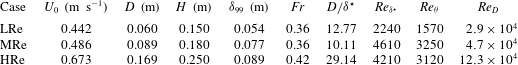
Due to limitations of the experimental facility, we had to obtain the selected levels of
 $\mathit{Re}_{D}$
by modifying both the pier diameter and the approach flow velocity (table 1). Practically, this means that each run was characterized by different boundary layer thicknesses (
$\mathit{Re}_{D}$
by modifying both the pier diameter and the approach flow velocity (table 1). Practically, this means that each run was characterized by different boundary layer thicknesses (
 ${\it\delta}_{99}$
) and channel blockage ratios. As mentioned in § 1, there is some evidence in the literature that the thickness of the boundary layer affects at least some aspects of junction flows (Ballio, Bettoni & Franzetti Reference Ballio, Bettoni and Franzetti1998; Simpson Reference Simpson2001; Roulund et al.
Reference Roulund, Sumer, Fredsøe and Michelsen2005). On the other hand, the influence of relatively thick boundary layers (
${\it\delta}_{99}$
) and channel blockage ratios. As mentioned in § 1, there is some evidence in the literature that the thickness of the boundary layer affects at least some aspects of junction flows (Ballio, Bettoni & Franzetti Reference Ballio, Bettoni and Franzetti1998; Simpson Reference Simpson2001; Roulund et al.
Reference Roulund, Sumer, Fredsøe and Michelsen2005). On the other hand, the influence of relatively thick boundary layers (
 ${\it\delta}_{99}>0.2D$
), like the ones in this study, is rather weak (Koken & Constantinescu Reference Koken and Constantinescu2009). In support of this statement, discrepancies in boundary layer thickness did not prevent recent numerical studies from reproducing important features of junction flows (Paik et al.
Reference Paik, Escauriaza and Sotiropoulos2007; Escauriaza & Sotiropoulos Reference Escauriaza and Sotiropoulos2011c
). For all three experimental runs the flow depths (
${\it\delta}_{99}>0.2D$
), like the ones in this study, is rather weak (Koken & Constantinescu Reference Koken and Constantinescu2009). In support of this statement, discrepancies in boundary layer thickness did not prevent recent numerical studies from reproducing important features of junction flows (Paik et al.
Reference Paik, Escauriaza and Sotiropoulos2007; Escauriaza & Sotiropoulos Reference Escauriaza and Sotiropoulos2011c
). For all three experimental runs the flow depths (
 $H$
) ensured that flow shallowness and flow patterns close to the free surface (superelevation of water surface, surface roller) have negligible effects on junction flow dynamics.
$H$
) ensured that flow shallowness and flow patterns close to the free surface (superelevation of water surface, surface roller) have negligible effects on junction flow dynamics.
Table 1. Major geometric and flow characteristics of the experimental set-ups.

As shown in figure 1, the primary flow measurements were performed at a streamwise–vertical plane located at the centreline of the upstream wall–cylinder junction. This region was selected because it: (i) is representative of the basic characteristics of junction flow, (ii) experiences minimum disturbances due to effects from the channel’s sidewalls, (iii) exhibits relatively small cross-plane fluid motion and (iv) provides a good reference for comparison with past studies. Flow measurements were also taken at the inlet of the test section for all three experiments. Streamwise and wall-normal velocity components were measured at a station located five diameters upstream of the leading edge of the cylinder. Again, the measurement plane was positioned on the centreline plane of symmetry. The same location was used for the characterization of the incoming boundary layers (refer to table 1 for the most important information regarding the boundary layer parameters, where
 ${\it\delta}^{\star }$
is the boundary layer displacement thickness and
${\it\delta}^{\star }$
is the boundary layer displacement thickness and
 ${\it\theta}$
the boundary layer momentum thickness).
${\it\theta}$
the boundary layer momentum thickness).
The fluid temperature was measured at various stations of the test section using a glass thermometer a few seconds before the initiation of data acquisition. It was found to be relatively constant at
 $23.5\pm 0.1\,^{\circ }\text{C}$
. Due to the small sampling duration, it can be safely assumed that this quantity remained constant throughout. The temperature differential between flowing water and surroundings was
$23.5\pm 0.1\,^{\circ }\text{C}$
. Due to the small sampling duration, it can be safely assumed that this quantity remained constant throughout. The temperature differential between flowing water and surroundings was
 $0.5\pm 0.1\,^{\circ }\text{C}$
, rendering negligible any effects induced by temperature-gradient advection (Allen & Naitoh Reference Allen and Naitoh2007).
$0.5\pm 0.1\,^{\circ }\text{C}$
, rendering negligible any effects induced by temperature-gradient advection (Allen & Naitoh Reference Allen and Naitoh2007).
2.2. Application of particle image velocimetry
We applied a fundamental implementation of the PIV technique, known as planar time-resolved particle image velocimetry (TRPIV). This generated multiple two-component velocity vectors over two-dimensional flow planes (2D2C version of PIV) with sufficient spatial and high temporal resolution. To control experimental errors, we closely followed as many best PIV practices as possible from those described in the excellent books by Raffel et al. (Reference Raffel, Willert, Wereley and Kompenhans2007) and Adrian & Westerweel (Reference Adrian and Westerweel2011). The same methodology was adopted for each experimental run. Therefore, we anticipate similar levels of errors and related uncertainties for all three
 $\mathit{Re}_{D}$
cases examined here. The good agreement we found between two replications of the MRe case attest to this statement. Next, we describe the outcomes of our efforts related to the use of PIV instrumentation, image processing and data analysis.
$\mathit{Re}_{D}$
cases examined here. The good agreement we found between two replications of the MRe case attest to this statement. Next, we describe the outcomes of our efforts related to the use of PIV instrumentation, image processing and data analysis.
2.2.1. Materials and PIV equipment
A basic premise in PIV is that tracing particles faithfully follow the paths of the water elements they displace. We seeded our flow with hollow glass particles. Their shape was nearly spherical, their mean diameter was
 $d_{p}=35~{\rm\mu}\text{m}$
, and their density had a nominal value of
$d_{p}=35~{\rm\mu}\text{m}$
, and their density had a nominal value of
 ${\it\rho}_{p}=1080~\text{kg}~\text{m}^{-3}$
. Whereas using particles heavier than water generally results in underestimation of the velocity magnitude, the particle properties used in this study were a compromise, selected to satisfy a variety of experimental constraints. The ratio of the particle response frequency (
${\it\rho}_{p}=1080~\text{kg}~\text{m}^{-3}$
. Whereas using particles heavier than water generally results in underestimation of the velocity magnitude, the particle properties used in this study were a compromise, selected to satisfy a variety of experimental constraints. The ratio of the particle response frequency (
 $t_{p}^{-1}$
) to that of the characteristic flow frequency is known as the particle Stokes number:
$t_{p}^{-1}$
) to that of the characteristic flow frequency is known as the particle Stokes number:
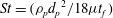 $\mathit{St}=({\it\rho}_{p}{d_{p}}^{2}/18{\it\mu}t_{f})$
, where
$\mathit{St}=({\it\rho}_{p}{d_{p}}^{2}/18{\it\mu}t_{f})$
, where
 ${\it\mu}$
is the dynamic viscosity of water and
${\it\mu}$
is the dynamic viscosity of water and
 $t_{f}$
is a time scale for the turbulent velocity fluctuations in the flow. Calculated
$t_{f}$
is a time scale for the turbulent velocity fluctuations in the flow. Calculated
 $\mathit{St}$
were 0.0086, 0.0098 and 0.0122 for the LRe, MRe and HRe cases, respectively, based on
$\mathit{St}$
were 0.0086, 0.0098 and 0.0122 for the LRe, MRe and HRe cases, respectively, based on
 $t_{f}$
values of
$t_{f}$
values of
 $9.2\times 10^{-3}$
,
$9.2\times 10^{-3}$
,
 $8.1\times 10^{-3}$
and
$8.1\times 10^{-3}$
and
 $6.5\times 10^{-3}~\text{s}$
. These values of
$6.5\times 10^{-3}~\text{s}$
. These values of
 $t_{f}$
are the characteristic turn-over times of the smallest, distinct and clearly identifiable vortices for each
$t_{f}$
are the characteristic turn-over times of the smallest, distinct and clearly identifiable vortices for each
 $\mathit{Re}$
case. They are considered representative of the time scales of flow fluctuations that are of particular interest in this study. On the other hand, the particle time scale had a value of
$\mathit{Re}$
case. They are considered representative of the time scales of flow fluctuations that are of particular interest in this study. On the other hand, the particle time scale had a value of
 $t_{p}=8.18\times 10^{-5}~\text{s}$
. It is, therefore, expected that seeding particles would respond with negligible lag to changes in the direction of the bulk flow.
$t_{p}=8.18\times 10^{-5}~\text{s}$
. It is, therefore, expected that seeding particles would respond with negligible lag to changes in the direction of the bulk flow.
A 20 W dual-cavity pulsed Nd:YLF laser was used to illuminate the flow. Each pulse had a wavelength of 527 nm, was fired at a frequency of 1000 Hz, and emitted a nominal energy of 10 mJ. Using a convex lens with a focal length of 50 mm, a spherical lens with a focal length of 300 mm, and a series of mirrors, the beam was delivered in the test section through the transparent bottom of the channel (figure 1). The thickness of the laser sheet was
 $2.0\pm 0.2~\text{mm}$
throughout the camera’s field of view. We selected this thickness to effectively deal with out-of-plane particle motion: an important source of error in PIV measurements.
$2.0\pm 0.2~\text{mm}$
throughout the camera’s field of view. We selected this thickness to effectively deal with out-of-plane particle motion: an important source of error in PIV measurements.
To achieve the desirable magnification of the region of interest, the distance between the centre of the camera lens and the CMOS sensor was adjusted using extension tubes. The optical axis of the lens was perpendicular to the channel’s sidewall to eliminate the unwanted effects stemming from refraction of light due to its propagation through different media (air, Plexiglas, water). The final geometric configuration resulted in a maximum error of 1.35 % affecting the outermost regions of the images due to deviations of the viewing angle from the optimum of
 $90^{\circ }$
. Autocorrelations of image intensities yielded an average diameter for the imaged particles of
$90^{\circ }$
. Autocorrelations of image intensities yielded an average diameter for the imaged particles of
 $d_{{\it\tau}}=2.3\pm 0.5~\text{pixel}$
. A value close or higher than two pixels has been reported as sufficient to drastically mitigate pixel-locking-induced errors (Raffel et al.
Reference Raffel, Willert, Wereley and Kompenhans2007; Adrian & Westerweel Reference Adrian and Westerweel2011).
$d_{{\it\tau}}=2.3\pm 0.5~\text{pixel}$
. A value close or higher than two pixels has been reported as sufficient to drastically mitigate pixel-locking-induced errors (Raffel et al.
Reference Raffel, Willert, Wereley and Kompenhans2007; Adrian & Westerweel Reference Adrian and Westerweel2011).
The resulting depth of field was
 $3.2\pm 0.2~\text{mm}$
(
$3.2\pm 0.2~\text{mm}$
(
 ${>}$
light sheet thickness, so that diffraction-limited images are captured) and the average magnification factor was equal to
${>}$
light sheet thickness, so that diffraction-limited images are captured) and the average magnification factor was equal to
 $63.52\pm 0.19~{\rm\mu}\text{m}/\text{pixel}$
. Particle motion was tracked with a
$63.52\pm 0.19~{\rm\mu}\text{m}/\text{pixel}$
. Particle motion was tracked with a
 $1.3\times 10^{6}~\text{pixel}$
high-speed camera, which was operated at a frequency of 1000 Hz. The inter-frame time of 1 ms assured maximum particle displacements between four and seven pixels for all
$1.3\times 10^{6}~\text{pixel}$
high-speed camera, which was operated at a frequency of 1000 Hz. The inter-frame time of 1 ms assured maximum particle displacements between four and seven pixels for all
 $\mathit{Re}$
cases. We selected the single-frame mode for PIV data acquisition to: (a) obtain maximum light intensity by the simultaneous firing of the two laser cavities, (b) maximize the number of collected images, and (c) minimize loss of correlation due to unequal exposures between consecutive images. As a result, 3270 frames filled the 4 GB-buffer of the camera for each
$\mathit{Re}$
cases. We selected the single-frame mode for PIV data acquisition to: (a) obtain maximum light intensity by the simultaneous firing of the two laser cavities, (b) maximize the number of collected images, and (c) minimize loss of correlation due to unequal exposures between consecutive images. As a result, 3270 frames filled the 4 GB-buffer of the camera for each
 $\mathit{Re}_{D}$
case. The total sampling time of 3.27 s corresponded to an average of
$\mathit{Re}_{D}$
case. The total sampling time of 3.27 s corresponded to an average of
 $24.5\pm 1.4$
characteristic times (
$24.5\pm 1.4$
characteristic times (
 $t_{c}={\it\delta}_{99}/U_{0}$
) of the incoming flows. The maximum available image resolution of
$t_{c}={\it\delta}_{99}/U_{0}$
) of the incoming flows. The maximum available image resolution of
 $1280~\text{pixel}\times 1024~\text{pixel}$
was used. Consequently, the average dimensions of the imaged flow field was the same for all three experiments,
$1280~\text{pixel}\times 1024~\text{pixel}$
was used. Consequently, the average dimensions of the imaged flow field was the same for all three experiments,
 $7.31~\text{cm}\times 5.62~\text{cm}$
.
$7.31~\text{cm}\times 5.62~\text{cm}$
.
2.2.2. Image preconditioning and analysis
Image preconditioning included the subtraction of the time-averaged mean image intensity from every frame (Honkanen & Nobach Reference Honkanen and Nobach2005). Additional enhancements were achieved by accurately defining the boundaries of the domain through gradient-based edge detection. To account for the undesirable contributions of some very bright particles in the resolution of the domain, we capped their intensity (Shavit, Lowe & Steinbuck Reference Shavit, Lowe and Steinbuck2007).
We adopted a common analysis procedure for all three
 $\mathit{Re}_{D}$
cases. PIV images were processed with software that implements the Robust Phase Correlation algorithm (Eckstein, Charonko & Vlachos Reference Eckstein, Charonko and Vlachos2008; Eckstein & Vlachos Reference Eckstein and Vlachos2009). Multi-grid, iterative and deformable windows were used to resolve the instantaneous flow fields. Three passes with two iterations in each were applied. The dimensions of the interrogation windows were reduced in each subsequent pass (from
$\mathit{Re}_{D}$
cases. PIV images were processed with software that implements the Robust Phase Correlation algorithm (Eckstein, Charonko & Vlachos Reference Eckstein, Charonko and Vlachos2008; Eckstein & Vlachos Reference Eckstein and Vlachos2009). Multi-grid, iterative and deformable windows were used to resolve the instantaneous flow fields. Three passes with two iterations in each were applied. The dimensions of the interrogation windows were reduced in each subsequent pass (from
 $64~\text{pixel}\times 64~\text{pixel}$
to
$64~\text{pixel}\times 64~\text{pixel}$
to
 $32~\text{pixel}\times 32~\text{pixel}$
to
$32~\text{pixel}\times 32~\text{pixel}$
to
 $16~\text{pixel}\times 16~\text{pixel}$
). Each window overlapped by 50 % with its adjacent ones in both
$16~\text{pixel}\times 16~\text{pixel}$
). Each window overlapped by 50 % with its adjacent ones in both
 $x$
and
$x$
and
 $y$
directions. Discrete Window Offsetting (Westerweel Reference Westerweel1997) accounted for the loss of correlation signal in the second pass due to in-plane particle motion. Vector validation was performed based on velocity thresholding and the Universal Outlier Detection technique (Westerweel & Scarano Reference Westerweel and Scarano2005). The percentage of valid vectors derived from the PIV image analysis ranged from 96.5 % to 99.7 %. The final processed velocity fields had a uniform vector grid spacing of
$y$
directions. Discrete Window Offsetting (Westerweel Reference Westerweel1997) accounted for the loss of correlation signal in the second pass due to in-plane particle motion. Vector validation was performed based on velocity thresholding and the Universal Outlier Detection technique (Westerweel & Scarano Reference Westerweel and Scarano2005). The percentage of valid vectors derived from the PIV image analysis ranged from 96.5 % to 99.7 %. The final processed velocity fields had a uniform vector grid spacing of
 $8~\text{pixel}\times 8~\text{pixel}$
. On average, the Eulerian representation of the instantaneous, two-dimensional flow field was obtained using 17 828 velocity vectors. The total number of measurements collected for all three
$8~\text{pixel}\times 8~\text{pixel}$
. On average, the Eulerian representation of the instantaneous, two-dimensional flow field was obtained using 17 828 velocity vectors. The total number of measurements collected for all three
 $\mathit{Re}_{D}$
cases was 174 889 410.
$\mathit{Re}_{D}$
cases was 174 889 410.
2.2.3. Data post-processing
Velocity derivatives were calculated using a compact fourth-order scheme with Richardson extrapolation. This hybrid operator has been shown to outperform conventional second-order finite difference schemes for the range of wavenumbers typically present in PIV data (Etebari & Vlachos Reference Etebari and Vlachos2005). Note, however, that some discrepancies in PIV vorticity data will always exist regardless of the selection of the differential operator. These stem from contributions of the very small turbulence scales that remain under-resolved (Wallace & Foss Reference Wallace and Foss1995). Since this work focuses on the behaviour of larger turbulence scales, we expect that this effect is negligible.
3. Results and discussion
The first part of the presentation and discussion of our results is devoted to the prominent features of the time-averaged flow fields. We discuss the effects of
 $\mathit{Re}_{D}$
on a number of turbulent statistics derived from the PIV data. Next, we probe into the time-dependent flow dynamics. The unsteady behaviour of the dominant flow patterns is analysed in an effort to reveal details that are filtered out, when averaged in time. Maps, tracking the trajectories of the primary horseshoe vortex in time, complement this discussion. Finally, we examine the p.d.f.s of velocity fluctuations to characterize the unsteady nature of the junction flows studied here.
$\mathit{Re}_{D}$
on a number of turbulent statistics derived from the PIV data. Next, we probe into the time-dependent flow dynamics. The unsteady behaviour of the dominant flow patterns is analysed in an effort to reveal details that are filtered out, when averaged in time. Maps, tracking the trajectories of the primary horseshoe vortex in time, complement this discussion. Finally, we examine the p.d.f.s of velocity fluctuations to characterize the unsteady nature of the junction flows studied here.
Most of the results are presented as maps of the spatial distribution of the parameter of interest on the measurement plane. The dimensions of the domain are scaled with the cylinder’s diameter. A constant area of
 $0.45D$
by
$0.45D$
by
 $0.35D$
is illustrated in every figure included in this paper. These are the maximum dimensions of the flow field that PIV imaging captured for the HRe case. Note, however, that due to: (i) the different cylinder diameters among cases and (ii) the constant spatial resolution of the measurements, the number of data points used to generate maps for each one of the three
$0.35D$
is illustrated in every figure included in this paper. These are the maximum dimensions of the flow field that PIV imaging captured for the HRe case. Note, however, that due to: (i) the different cylinder diameters among cases and (ii) the constant spatial resolution of the measurements, the number of data points used to generate maps for each one of the three
 $\mathit{Re}_{D}$
experiments is not the same. Whenever required, results are non-dimensionalized with the approach velocity or the characteristic time of the incoming flow. An asterisk is used to indicate dimensionless parameters. The convention that water flows from left to right is adopted (figure 1). The leading edges of the cylinders are drawn as grey rectangles on the right of each figure. To avoid cluttering of the images, we do not show every vector available. The origin of the Cartesian coordinate system is located at the intersection of the leading edge of the pier with the bed. The orientation of the coordinate system is as follows (positive directions):
$\mathit{Re}_{D}$
experiments is not the same. Whenever required, results are non-dimensionalized with the approach velocity or the characteristic time of the incoming flow. An asterisk is used to indicate dimensionless parameters. The convention that water flows from left to right is adopted (figure 1). The leading edges of the cylinders are drawn as grey rectangles on the right of each figure. To avoid cluttering of the images, we do not show every vector available. The origin of the Cartesian coordinate system is located at the intersection of the leading edge of the pier with the bed. The orientation of the coordinate system is as follows (positive directions):
 $x$
coincides with that of the approach flow,
$x$
coincides with that of the approach flow,
 $y$
is towards the free surface, and
$y$
is towards the free surface, and
 $z$
points to the camera.
$z$
points to the camera.
3.1. Time-averaged junction flow characteristics
We superimpose the time-averaged streamlines on non-dimensionalized velocity contour plots for each
 $\mathit{Re}_{D}$
case in figure 2(a–c). The junction region is home to two characteristic flow structures that manifest in the form of closed streamlines of a roughly elliptical or spiral pattern. We refer to the horseshoe vortex closer to the pier as HV1 (or primary) and the vortex further upstream as HV2 (or secondary). Their locations are not identical for every
$\mathit{Re}_{D}$
case in figure 2(a–c). The junction region is home to two characteristic flow structures that manifest in the form of closed streamlines of a roughly elliptical or spiral pattern. We refer to the horseshoe vortex closer to the pier as HV1 (or primary) and the vortex further upstream as HV2 (or secondary). Their locations are not identical for every
 $\mathit{Re}_{D}$
experiment. The core of HV1 is centred around (
$\mathit{Re}_{D}$
experiment. The core of HV1 is centred around (
 $-0.14D$
,
$-0.14D$
,
 $0.04D$
), (
$0.04D$
), (
 $-0.19D$
,
$-0.19D$
,
 $0.06D$
) and (
$0.06D$
) and (
 $-0.17D$
,
$-0.17D$
,
 $0.05D$
), respectively, for the cases of LRe, MRe and HRe. The coordinates for the corresponding cores of HV2 are (
$0.05D$
), respectively, for the cases of LRe, MRe and HRe. The coordinates for the corresponding cores of HV2 are (
 $-0.32$
, 0.01), (
$-0.32$
, 0.01), (
 $-0.36$
, 0.02) and (
$-0.36$
, 0.02) and (
 $-0.29$
, 0.01). These results suggest that the spatial variability regarding the position of the cores is higher for the horizontal direction. Nevertheless, and in contrast to the findings of Agui & Andreopoulos (Reference Agui and Andreopoulos1992), they do not support a clear trend regarding the location of the vortices as we move from smaller to higher levels of
$-0.29$
, 0.01). These results suggest that the spatial variability regarding the position of the cores is higher for the horizontal direction. Nevertheless, and in contrast to the findings of Agui & Andreopoulos (Reference Agui and Andreopoulos1992), they do not support a clear trend regarding the location of the vortices as we move from smaller to higher levels of
 $\mathit{Re}_{D}$
. Differences with respect to the relative horizontal distances between HV1 and HV2 are also notable. These are
$\mathit{Re}_{D}$
. Differences with respect to the relative horizontal distances between HV1 and HV2 are also notable. These are
 $0.18D$
and
$0.18D$
and
 $0.17D$
for LRe and MRe, but only
$0.17D$
for LRe and MRe, but only
 $0.12D$
for HRe. The proximity between HV1 and HV2 for the latter case facilitates their interaction.
$0.12D$
for HRe. The proximity between HV1 and HV2 for the latter case facilitates their interaction.

Figure 2. Spatial distribution of time-averaged streamlines and non-dimensionalized velocity magnitude,
 $\Vert U\Vert$
. Two vortex cores, named as HV1 (right) and HV2 (left), appear regardless of
$\Vert U\Vert$
. Two vortex cores, named as HV1 (right) and HV2 (left), appear regardless of
 $\mathit{Re}_{D}$
(a–c).
$\mathit{Re}_{D}$
(a–c).
The most striking feature of the streamline fields in figure 2 is the clarity and distinctiveness of the vortices and the number of streamlines captured by or contained within the vortices (particularly HV1). This clarity is greatest for the HRe case. This is consistent with the instantaneous flow fields, which are discussed later, in that vortices of the LRe and MRe cases are more intermittent in nature and exhibit larger variability in their location and movement (see for example figure 19 in § 3.3.1). Here we will use the streamline topology to examine the relationship between the two dominant vortices in the time-averaged domain and the return flow of fluid after it impinges on the cylinder’s face. A comparison between the HV2 of LRe and MRe shows that the former captures fewer streamlines (and in fact less fluid mass) than the latter. The return flow is stronger for MRe, with both the primary and secondary vortices in this case benefiting from the influx of mass and momentum of fluid deflected on the obstacle’s leading edge (figure 2
b). The trend of increasing intensity of return flow with
 $\mathit{Re}_{D}$
is valid for HRe too. However, our data show that for this case streamlines of deflected fluid feed exclusively the primary vortex.
$\mathit{Re}_{D}$
is valid for HRe too. However, our data show that for this case streamlines of deflected fluid feed exclusively the primary vortex.
Focusing on the area between HV1 and HV2, the streamline topology does not suggest the presence of a tertiary vortex (HV3). This appears to contradict results from topological models inferred through flow visualizations (Baker Reference Baker1979; Dargahi Reference Dargahi1989; Simpson Reference Simpson2001). According to these studies, vorticity extracted from the wall below HV1 reorganizes to form a counterclockwise vortex at the saddle region between HV1 and HV2. We postulate that the absence of this flow pattern for the levels of
 $\mathit{Re}_{D}$
investigated here stems from the highly unsteady behaviour of the flow in this particular region. As we will elaborate in subsequent sections of the paper using animations of TRPIV data, a tertiary vortex does frequently appear but undergoes various cycles of upliftings, eruptions and amalgamations with other vortices in a seemingly random fashion (refer to the work by Agui & Andreopoulos (Reference Agui and Andreopoulos1992) for descriptions of similar phenomena). This unsteadiness is filtered out, when time-averaged representations of the flow field are investigated.
$\mathit{Re}_{D}$
investigated here stems from the highly unsteady behaviour of the flow in this particular region. As we will elaborate in subsequent sections of the paper using animations of TRPIV data, a tertiary vortex does frequently appear but undergoes various cycles of upliftings, eruptions and amalgamations with other vortices in a seemingly random fashion (refer to the work by Agui & Andreopoulos (Reference Agui and Andreopoulos1992) for descriptions of similar phenomena). This unsteadiness is filtered out, when time-averaged representations of the flow field are investigated.
Another notable topological characteristic is the absence of CV very close to the intersection of the wall with the cylinder. In the literature, the existence of such a vortex is attributed to the separation of fluid running down the cylinder’s face due to the adverse pressure gradient imposed by the wall. Here, curved streamlines for the MRe and HRe cases provide inconclusive evidence about the presence of CV in a time-averaged sense. Insufficient spatial resolution of our measurements or the increased uncertainty for the data close to solid boundaries are plausible explanations for this discrepancy. However, a careful frame-by-frame inspection of the instantaneous flow fields does not support this conjecture. Corner vortices in the form of properly closed streamlines were observed for all
 $\mathit{Re}_{D}$
cases in the instantaneous flow field measurements. They emerged and disappeared intermittently with insufficient frequency and structure to survive the averaging process resulting in the features of figure 2.
$\mathit{Re}_{D}$
cases in the instantaneous flow field measurements. They emerged and disappeared intermittently with insufficient frequency and structure to survive the averaging process resulting in the features of figure 2.
Overall, our results for the time-averaged flow topology are in good agreement with those of past studies (Praisner & Smith Reference Praisner and Smith2006b
; Paik et al.
Reference Paik, Escauriaza and Sotiropoulos2007; Kirkil & Constantinescu Reference Kirkil and Constantinescu2009; Sabatino & Smith Reference Sabatino and Smith2009). The two-vortex model was verified for the studied
 $\mathit{Re}_{D}$
levels, which range between
$\mathit{Re}_{D}$
levels, which range between
 $\simeq 3\times 10^{4}$
and
$\simeq 3\times 10^{4}$
and
 $12\times 10^{4}$
. The only inconsistency with some of the aforementioned works is with respect to the absence of the CV.
$12\times 10^{4}$
. The only inconsistency with some of the aforementioned works is with respect to the absence of the CV.
Apart from the topological characteristics of the flow, figure 2(a–c) provides insight on the spatial distribution of flow momentum. Generally, incoming flow enters the junction region at levels close to 60 % of the bulk velocity and decelerates as it approaches the solid boundaries. An exception to flow retardation occurs within the region below HV1. There, high-momentum fluid is associated with the strong near-wall jet of reversed flow (Devenport & Simpson Reference Devenport and Simpson1990; Paik et al.
Reference Paik, Escauriaza and Sotiropoulos2007; Kirkil & Constantinescu Reference Kirkil and Constantinescu2009). Our measurements reveal that the increase in
 $\mathit{Re}_{D}$
makes this feature more pronounced, as evidenced by the amplified velocity magnitudes. For the HRe case, fluid of higher momentum (visualized by red-coloured bands) penetrates regions near the corner (figure 2
c) and HV1 is located closer to the bottom wall. The proximity between the lower part of the vortex and the solid boundary eventually results in the contraction of streamlines comprising the near-wall jet of reversed flow and in the increase of flow velocities. In subsequent discussions about the time-averaged distribution of vorticity and the instantaneous flow fields, we will demonstrate that this feature has further implications for the flow physics dominated by vortex–wall interactions.
$\mathit{Re}_{D}$
makes this feature more pronounced, as evidenced by the amplified velocity magnitudes. For the HRe case, fluid of higher momentum (visualized by red-coloured bands) penetrates regions near the corner (figure 2
c) and HV1 is located closer to the bottom wall. The proximity between the lower part of the vortex and the solid boundary eventually results in the contraction of streamlines comprising the near-wall jet of reversed flow and in the increase of flow velocities. In subsequent discussions about the time-averaged distribution of vorticity and the instantaneous flow fields, we will demonstrate that this feature has further implications for the flow physics dominated by vortex–wall interactions.
Next, we analyse the time-averaged velocity field into its streamwise and wall-normal components (figure 3
a–c). In all three maps, two alternating regions of positive and negative wall-normal velocities (
 $V/U_{0}$
) bound the left and right outer edges of HV1. These flow patterns are absent for HV2, implying a difference between the behaviour of HV1 and HV2. This difference is consistent for all
$V/U_{0}$
) bound the left and right outer edges of HV1. These flow patterns are absent for HV2, implying a difference between the behaviour of HV1 and HV2. This difference is consistent for all
 $\mathit{Re}_{D}$
cases. Furthermore, flooded contour maps of
$\mathit{Re}_{D}$
cases. Furthermore, flooded contour maps of
 $V/U_{0}$
more clearly display the existence of a strong downwash of fluid (or downflow) at the face of the cylinder for MRe. Both the origin of this feature and its effect on the time-averaged flow elude a straightforward interpretation.
$V/U_{0}$
more clearly display the existence of a strong downwash of fluid (or downflow) at the face of the cylinder for MRe. Both the origin of this feature and its effect on the time-averaged flow elude a straightforward interpretation.

Figure 3. Contour lines of time-averaged streamwise velocity component superimposed on flood contour maps of time-averaged wall-normal component. Both parameters are non-dimensionalized with the approach velocity,
 $U_{0}$
.
$U_{0}$
.
Out-of-plane (or spanwise) vorticity (
 ${\it\omega}_{z}$
) plays a central role in the interpretation of junction flows. Recall that the reorganization of vorticity within the separated boundary layer contributes to the generation of horseshoe vortices. Time-averaged maps (figure 4
a–c) of this parameter attest to this statement. The colour-coding of the maps was chosen to highlight only areas of significant positive (red) and negative (blue) values. Pockets of high negative vorticity overlap with the cores of the primary vortices. On the other hand, the secondary eddies do not exhibit this feature. Their vortical content is an order of magnitude smaller than that of the primary vortices. Thus, it is difficult to distinguish between the vorticity of HV2 and the incoming vorticity of the separated shear flow. Our measurements elucidate the spatial connections between these latter trails of incoming vorticity (indicated by the arrow on figure 4
a) and the core of the primary vortex. This characteristic is particularly evident for the LRe and HRe cases (figure 4
a,c). For MRe, such a connection is weakly supported (figure 4
b). Instead, this case is characterized by another vertical patch of negative vorticity, which emanates from the downflow at the cylinder’s face and merges with the core of HV1. This patch runs on top of a thinner and longer streak of positive vorticity, whose magnitude becomes larger with
${\it\omega}_{z}$
) plays a central role in the interpretation of junction flows. Recall that the reorganization of vorticity within the separated boundary layer contributes to the generation of horseshoe vortices. Time-averaged maps (figure 4
a–c) of this parameter attest to this statement. The colour-coding of the maps was chosen to highlight only areas of significant positive (red) and negative (blue) values. Pockets of high negative vorticity overlap with the cores of the primary vortices. On the other hand, the secondary eddies do not exhibit this feature. Their vortical content is an order of magnitude smaller than that of the primary vortices. Thus, it is difficult to distinguish between the vorticity of HV2 and the incoming vorticity of the separated shear flow. Our measurements elucidate the spatial connections between these latter trails of incoming vorticity (indicated by the arrow on figure 4
a) and the core of the primary vortex. This characteristic is particularly evident for the LRe and HRe cases (figure 4
a,c). For MRe, such a connection is weakly supported (figure 4
b). Instead, this case is characterized by another vertical patch of negative vorticity, which emanates from the downflow at the cylinder’s face and merges with the core of HV1. This patch runs on top of a thinner and longer streak of positive vorticity, whose magnitude becomes larger with
 $\mathit{Re}_{D}$
.
$\mathit{Re}_{D}$
.

Figure 4. Maps of time-averaged spanwise vorticity for the various
 $\mathit{Re}_{D}$
cases. Arrow indicates the trail of incoming vorticity. Vorticities are non-dimensionalized with
$\mathit{Re}_{D}$
cases. Arrow indicates the trail of incoming vorticity. Vorticities are non-dimensionalized with
 $t_{c}$
.
$t_{c}$
.
Another structure that calls for attention is the horizontal sheet of positive vorticity below HV1. This layer originates at
 $0.06D$
for LRe and
$0.06D$
for LRe and
 $0.04D$
for both MRe and HRe. It extends respectively up to
$0.04D$
for both MRe and HRe. It extends respectively up to
 $0.20D$
,
$0.20D$
,
 $0.25D$
and
$0.25D$
and
 $0.24D$
. Its spatial extent implies that positive, near-wall vorticity is associated exclusively with HV1. The comparison of subplots in figure 4(a–c) also shows that near-wall vorticity remains attached to the bed only for the LRe case. The trend of increasing vorticity as we move to higher levels of
$0.24D$
. Its spatial extent implies that positive, near-wall vorticity is associated exclusively with HV1. The comparison of subplots in figure 4(a–c) also shows that near-wall vorticity remains attached to the bed only for the LRe case. The trend of increasing vorticity as we move to higher levels of
 $\mathit{Re}_{D}$
is verified here too. Positive vorticity eventually reaches levels comparable to the absolute value of those measured inside the core of HV1. Of interest is the relationship between the horizontal layer of positive vorticity below HV1 with the vertical layer of vorticity running down the leading edge of the cylinder. Figure 4(a–c) does not support an unambiguous connection between these two structures (at least on a time-averaged sense). This argument indicates that the horizontal, near-wall layer of positive vorticity stems primarily from the interaction between the HV1 and the wall (Paik et al.
Reference Paik, Escauriaza and Sotiropoulos2007). Our data suggest that the interaction is stronger for HRe case. This finding brings closure to the previous discussion on the position of HV1 and the topology of its streamlines. In summary, we invoked here the physics of the flow to establish a link between the momentum and vortical contents of junction flows.
$\mathit{Re}_{D}$
is verified here too. Positive vorticity eventually reaches levels comparable to the absolute value of those measured inside the core of HV1. Of interest is the relationship between the horizontal layer of positive vorticity below HV1 with the vertical layer of vorticity running down the leading edge of the cylinder. Figure 4(a–c) does not support an unambiguous connection between these two structures (at least on a time-averaged sense). This argument indicates that the horizontal, near-wall layer of positive vorticity stems primarily from the interaction between the HV1 and the wall (Paik et al.
Reference Paik, Escauriaza and Sotiropoulos2007). Our data suggest that the interaction is stronger for HRe case. This finding brings closure to the previous discussion on the position of HV1 and the topology of its streamlines. In summary, we invoked here the physics of the flow to establish a link between the momentum and vortical contents of junction flows.
The non-dimensionalized TKE is calculated from the PIV data as
 $\text{TKE}=((u^{\prime })^{2}+(v^{\prime })^{2})/(2U_{0}^{2})$
, where
$\text{TKE}=((u^{\prime })^{2}+(v^{\prime })^{2})/(2U_{0}^{2})$
, where
 $u^{\prime }$
and
$u^{\prime }$
and
 $v^{\prime }$
are the root-mean-square (r.m.s.) of the fluctuations of the streamwise and wall-normal velocity components. Within the junction region, TKE approximately peaks within the cores of HV1 (figure 5). At these locations, TKE progressively grows to levels an order of magnitude higher than those characterizing surrounding flow. A nearly horizontal trail of TKE emanates from the line of flow separation (not shown in presented figures), lifts off the wall, and wraps around the periphery of HV1. Another vertical trail of TKE feeds HV1, but this happens only for the LRe and MRe cases. For the latter, increased TKE levels were measured at the very corner between the wall and the cylinder. Related to the previous discussion, the implication here is that the CV could exhibit high turbulence energies, despite its weak manifestation on time-averaged plots.
$v^{\prime }$
are the root-mean-square (r.m.s.) of the fluctuations of the streamwise and wall-normal velocity components. Within the junction region, TKE approximately peaks within the cores of HV1 (figure 5). At these locations, TKE progressively grows to levels an order of magnitude higher than those characterizing surrounding flow. A nearly horizontal trail of TKE emanates from the line of flow separation (not shown in presented figures), lifts off the wall, and wraps around the periphery of HV1. Another vertical trail of TKE feeds HV1, but this happens only for the LRe and MRe cases. For the latter, increased TKE levels were measured at the very corner between the wall and the cylinder. Related to the previous discussion, the implication here is that the CV could exhibit high turbulence energies, despite its weak manifestation on time-averaged plots.

Figure 5. Non-dimensionalized TKE. Subfigure (c) exhibits two characteristic peaks of TKE.

Figure 6. Contour lines of streamwise turbulence intensity,
 $u^{\prime }/U_{0}$
, drawn on top of flood contour maps of wall-normal turbulence intensity,
$u^{\prime }/U_{0}$
, drawn on top of flood contour maps of wall-normal turbulence intensity,
 $v^{\prime }/U_{0}$
.
$v^{\prime }/U_{0}$
.
Comparison of the plots in figure 5(a–c) reveals an additional difference between the investigated flows. In particular, the HRe case exhibits a second peak of high TKE closer to the wall (figure 5
c). The distribution of TKE for MRe around HV1 is somewhat similar; yet the intensity near the bed is not high enough to generate a distinct secondary peak. This feature is absent from figure 5(a). Two peaks of TKE have been reported in previous experimental (Devenport & Simpson Reference Devenport and Simpson1990) and numerical studies (Paik et al.
Reference Paik, Escauriaza and Sotiropoulos2007; Kirkil & Constantinescu Reference Kirkil and Constantinescu2009; Escauriaza & Sotiropoulos Reference Escauriaza and Sotiropoulos2011c
). More specifically, Paik et al. (Reference Paik, Escauriaza and Sotiropoulos2007) were the first to establish a link between this second peak of TKE with the unsteady and bimodal behaviour of HV1. Note, however, that there are also differences between our results and those of the aforementioned works regarding this feature. For example, we found that the second patch of increased TKE is inclined with respect to the wall, whereas in the referenced studies it develops parallel to the solid boundary. An additional discrepancy is with respect to the investigated levels of
 $\mathit{Re}_{D}$
. In addition, Kirkil & Constantinescu (Reference Kirkil and Constantinescu2009, p. 9) calculated a double-peaked TKE structure for the flow around a cylinder at
$\mathit{Re}_{D}$
. In addition, Kirkil & Constantinescu (Reference Kirkil and Constantinescu2009, p. 9) calculated a double-peaked TKE structure for the flow around a cylinder at
 $\mathit{Re}_{D}=1.8\times 10^{4}$
. Escauriaza & Sotiropoulos (Reference Escauriaza and Sotiropoulos2011c
, p. 247) reported a C-shaped structure for DES simulations at
$\mathit{Re}_{D}=1.8\times 10^{4}$
. Escauriaza & Sotiropoulos (Reference Escauriaza and Sotiropoulos2011c
, p. 247) reported a C-shaped structure for DES simulations at
 $\mathit{Re}_{D}=3.9\times 10^{4}$
. Both of these levels of
$\mathit{Re}_{D}=3.9\times 10^{4}$
. Both of these levels of
 $\mathit{Re}_{D}$
are below our MRe case. Notwithstanding the limitations that obscure a straightforward comparison, this difference provides novel insight into the effects of
$\mathit{Re}_{D}$
are below our MRe case. Notwithstanding the limitations that obscure a straightforward comparison, this difference provides novel insight into the effects of
 $\mathit{Re}_{D}$
on turbulent junction flows.
$\mathit{Re}_{D}$
on turbulent junction flows.

Figure 7. Contour maps of time-averaged, non-dimensionalized Reynolds shear stresses for the various
 $\mathit{Re}_{D}$
cases.
$\mathit{Re}_{D}$
cases.
The analysis of the time-averaged characteristics of the junction flows under consideration also includes the discussion about the levels of turbulence. Figure 6(a–c) shows the spatial relationships between the streamwise and wall-normal turbulence intensities. A striking similarity among
 $\mathit{Re}_{D}$
cases is that
$\mathit{Re}_{D}$
cases is that
 $u^{\prime }/U_{0}$
and
$u^{\prime }/U_{0}$
and
 $v^{\prime }/U_{0}$
have nearly identical ranges. Consistent with previously presented results, the maximum concentration of turbulence intensity is located in the neighbourhood of HV1. This is an additional testament to the degree of unsteadiness of the primary vortex. Higher levels of
$v^{\prime }/U_{0}$
have nearly identical ranges. Consistent with previously presented results, the maximum concentration of turbulence intensity is located in the neighbourhood of HV1. This is an additional testament to the degree of unsteadiness of the primary vortex. Higher levels of
 $u^{\prime }/U_{0}$
characterize HRe. For this case, streamwise turbulence intensity peaks at two locations: the core of the vortex and the region between the bottom periphery of the vortex and the bed. The shape of the HRe contours is similar to that of TKE (figure 5
c). Interestingly, this analogy is not present for the other two cases. Although contour lines in figure 6(a,b) support the existence of a double-peak structure (or even a triple peak for LRe), this feature is absent in figure 5(a,b). We conclude, therefore, that the relative contribution of the near-wall jet becomes more substantial at higher levels of
$u^{\prime }/U_{0}$
characterize HRe. For this case, streamwise turbulence intensity peaks at two locations: the core of the vortex and the region between the bottom periphery of the vortex and the bed. The shape of the HRe contours is similar to that of TKE (figure 5
c). Interestingly, this analogy is not present for the other two cases. Although contour lines in figure 6(a,b) support the existence of a double-peak structure (or even a triple peak for LRe), this feature is absent in figure 5(a,b). We conclude, therefore, that the relative contribution of the near-wall jet becomes more substantial at higher levels of
 $\mathit{Re}_{D}$
. Finally, it was not possible to establish a meaningful connection between the region of reduced turbulence at the upper left corner of figure 6(a) and the dynamics of the horseshoe vortex system.
$\mathit{Re}_{D}$
. Finally, it was not possible to establish a meaningful connection between the region of reduced turbulence at the upper left corner of figure 6(a) and the dynamics of the horseshoe vortex system.
Lastly, and for completeness, the contour maps for the dimensionless covariance,
 $-\langle uv\rangle ^{\ast }$
, or kinematic Reynolds shear stress, are shown in figure 7(a–c). It is observed that the range of the stress is comparable for all three
$-\langle uv\rangle ^{\ast }$
, or kinematic Reynolds shear stress, are shown in figure 7(a–c). It is observed that the range of the stress is comparable for all three
 $\mathit{Re}_{D}$
cases and that the extremes are confined to the regions near the face of the cylinder – and more strikingly in the vicinity of the primary vortex. Near the primary vortex, two islands in the contour map are apparent for all
$\mathit{Re}_{D}$
cases and that the extremes are confined to the regions near the face of the cylinder – and more strikingly in the vicinity of the primary vortex. Near the primary vortex, two islands in the contour map are apparent for all
 $\mathit{Re}_{D}$
cases. Comparing these maps with the mean-velocity field structure (figure 2), it is observed that the positive Reynolds shear stress peak is positioned within the region of the primary vortex core, where the mean-velocity gradient is very high, particularly near the centre of the vortex. This is consistent with the shear stress profiles measured by Devenport & Simpson (Reference Devenport and Simpson1990). The large negative shear stress zone occurs in the saddle region between the primary and secondary vortices. These two high-stress regions are larger and more distinct for the HRe case.
$\mathit{Re}_{D}$
cases. Comparing these maps with the mean-velocity field structure (figure 2), it is observed that the positive Reynolds shear stress peak is positioned within the region of the primary vortex core, where the mean-velocity gradient is very high, particularly near the centre of the vortex. This is consistent with the shear stress profiles measured by Devenport & Simpson (Reference Devenport and Simpson1990). The large negative shear stress zone occurs in the saddle region between the primary and secondary vortices. These two high-stress regions are larger and more distinct for the HRe case.
3.2. Time-resolved dynamics of junction flows
Particle image velocimetry allows a global representation of the flow field at discrete time instants. We took advantage of this capability and carried out a frame-by-frame analysis. A wealth of flow patterns was revealed. It is beyond the scope of this work to present a detailed appraisal of every instantaneous topology mapped on the measurement plane. Instead, we emphasize flow episodes that elucidate important aspects of the dynamic behaviour of the horseshoe vortex for the various
 $\mathit{Re}_{D}$
levels. We complement our discussion with sequences of characteristic snapshots. The analysis highlights important similarities and distinct differences that collectively portray the effects of
$\mathit{Re}_{D}$
levels. We complement our discussion with sequences of characteristic snapshots. The analysis highlights important similarities and distinct differences that collectively portray the effects of
 $\mathit{Re}_{D}$
on the turbulent flows at wall–cylinder junctions. Whenever possible, we compare our findings with those of past studies.
$\mathit{Re}_{D}$
on the turbulent flows at wall–cylinder junctions. Whenever possible, we compare our findings with those of past studies.
3.2.1. Case of
 $\mathit{Re}_{D}=2.9\times 10^{4}$
(LRe)
$\mathit{Re}_{D}=2.9\times 10^{4}$
(LRe)

The time-resolved analysis of flow dynamics for the LRe case revealed numerous flow patterns that were not detectable in the time-averaged velocity signals. High levels of intermittency characterize this junction flow, manifested in both large (organized vortices) and small-scale flow components (near-wall fluid flow). For example, we discovered that the junction region is home to a number of vortices ranging from one to four (figure 8 a,b). Vortex stretching and meandering increase the spatial extent of the orbits followed by the vortex cores. It is possible, therefore, that the secondary vortex (HV2) shown in the topology of figure 2 is just the average expression of a number of vortices, instead of a unique flow structure. More confidence exists in the expression of the primary vortex, although its presence on the flow field is not continuous.

Figure 8. Characteristic instantaneous flow topologies for the LRe case showing: (a) the minimum and (b) the maximum number of vortices.
The occasional disintegration of HV1 is a feature for which no hint was provided for by the time-averaged analysis. It was the frame-by-frame inspection of the flow field for the LRe case that revealed it. For a significant number of frames, the flow topology was devoid of the primary horseshoe vortex. These snapshots were clustered in thirteen groups. Their total duration was 440 ms, representing 13.5 % of the LRe experiment. The disappearance of HV1 is interpreted as a loss of its coherence. Figure 9(a–d) shows that this state is preceded by the collision of HV1 with a fluid patch originating from the downwash flow parallel to the obstacle. This mechanism could offer a plausible explanation for the obliteration of HV1, because it was identified in the majority of the episodes (eight out of thirteen). The absence of this or another possible mechanism (Paik et al. Reference Paik, Escauriaza and Sotiropoulos2007) for the remaining five episodes, however, casts doubts on the generality of that conclusion. Regardless of the origin of the phenomenon, the unsteadiness in the region formerly occupied by the core of HV1 is substantial (figure 9 c). The flow dynamics locally appear to assume an erratic behaviour, with changes in topology occurring even faster than the sampling rate of 1000 Hz. This also prohibits drawing sound conclusions about what brings about the end of the unsteadiness and re-stabilizes the flow, which then returns to more easily identifiable patterns (figure 9 d). Note that during the absence of HV1, the secondary vortex retains its coherence and relative position within the flow topology.

Figure 9. Sequence of snapshots displaying the disintegration of HV1 for the LRe case. Flood contour maps express the magnitude of the wall-normal velocity component. Dimensionless time is indicated by the value of
 $t^{\ast }$
: (a)
$t^{\ast }$
: (a)
 $t^{\ast }=7.43$
, (b)
$t^{\ast }=7.43$
, (b)
 $t^{\ast }=7.53$
, (c)
$t^{\ast }=7.53$
, (c)
 $t^{\ast }=7.63$
, (d)
$t^{\ast }=7.63$
, (d)
 $t^{\ast }=7.73$
.
$t^{\ast }=7.73$
.
The discussion on the dynamics of the primary horseshoe vortex is extended to include interactions with HV2. In the absence of the tertiary vortex, there is a direct interplay between HV1 and HV2. Figure 10(a–d) demonstrates a sequence of snapshots describing an episode that ends up with the amalgamation of the vortices. In the beginning (figure 10 a), the two cores are close together. In a subsequent frame (figure 10 b), the two structures share a number of common streamlines at the lower edges of their peripheries. The interaction becomes closer, so that both cores are surrounded by the same outer streamlines (figure 10 c). Observe also the appearance of a new, transient structure in the vicinity of the cylinder. Finally, the two vortices merge into a single, large-scale structure (figure 10 d).

Figure 10. Amalgamation of HV1 with HV2: (a)
 $t^{\ast }=7.85$
, (b)
$t^{\ast }=7.85$
, (b)
 $t^{\ast }=7.87$
, (c)
$t^{\ast }=7.87$
, (c)
 $t^{\ast }=7.93$
, (d)
$t^{\ast }=7.93$
, (d)
 $t^{\ast }=8.08$
.
$t^{\ast }=8.08$
.
Next, we revisit the bimodal dynamics of the horseshoe vortex motivated by the prominent position of this subject in the junction flow literature (Devenport & Simpson Reference Devenport and Simpson1990; Paik et al. Reference Paik, Escauriaza and Sotiropoulos2007; Kirkil & Constantinescu Reference Kirkil and Constantinescu2009). Instantaneous representations of the global velocity field simplify flow classification. Thus, there is no need to resort to indirect methodologies (like the one devised by Devenport & Simpson (Reference Devenport and Simpson1990) for data collected with point-wise velocity measuring techniques) to determine the characteristic modes and the time spent by the flow in each one of them. A painstaking examination of the cinematography of the PIV data suffices for a direct and unambiguous detection of these modes.
A noteworthy finding of our analysis is that zeroflow and backflow are not the only modes that characterize junction flows. For a significant number of frames, the characteristics of the flow field do not verify the topologies of any of these two well-known modes. Figure 11(a–c) juxtaposes three snapshots representative of the backflow, the zeroflow and this other mode, which we will refer to from now on as intermediate. The backflow mode is characterized by a strong near-wall jet, which moves against the bulk flow (figure 11 c). On the other hand, zeroflow mode occurs when the motion of the jet is impeded (figure 11 a). The reverse flow is then directed upwards at high velocities. These descriptions are in good agreement with the original definitions provided by Devenport & Simpson (Reference Devenport and Simpson1990) and have been corroborated by subsequent studies (Paik et al. Reference Paik, Escauriaza and Sotiropoulos2007; Kirkil & Constantinescu Reference Kirkil and Constantinescu2009; Gand et al. Reference Gand, Deck, Brunet and Sagaut2010). Differences also emerge through this comparison. The most striking of them is that, in contrast to what has been suggested in the literature, the flow modes do not have preferential locations within the flow domain. For example, in figure 11(c) one would have expected the appearance of zeroflow, because the primary horseshoe vortex is located very close to the cylinder. Nevertheless, the backflow mode is clearly present. As far as the intermediate mode is concerned, it collectively symbolizes every flow topology that does not fall into one of the well-known categories. Although there are various expressions of the intermediate mode, figure 11(b) highlights a typical one. It is observed that the interface between the incoming and return flow does not form a vertical line. The rather weak return flow separates from the bed and is directed upwards, but is lacking the momentum required to propagate further upstream. Its path terminates upon its encountering with the incoming flow. Unlike the zeroflow mode, the incoming flow here is not strong enough to cause the vertical ejection of fluid at high velocities. Essentially, the momentum of the return flow is diffused within its surroundings. Previous studies have mentioned the possibility of existence for additional junction flows modes, but did not elaborate further on the subject (Devenport & Simpson Reference Devenport and Simpson1990; Praisner & Smith Reference Praisner and Smith2006a ). The intermediate mode indicates that the switching between the two modes is not continuous. This could potentially suggest modifications in the nature of phenomena that have been linked to the mode-switching mechanism (Agui & Andreopoulos Reference Agui and Andreopoulos1992; Ölçmen & Simpson Reference Ölçmen and Simpson1994; Praisner et al. Reference Praisner, Seal, Takmaz and Smith1997; Kirkil & Constantinescu Reference Kirkil and Constantinescu2009; Escauriaza & Sotiropoulos Reference Escauriaza and Sotiropoulos2011a ,Reference Escauriaza and Sotiropoulos b ).
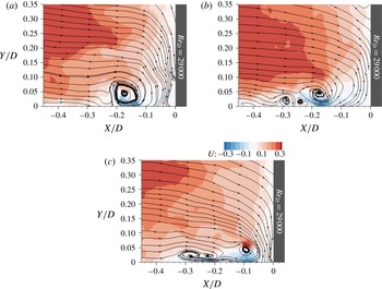
Figure 11. Characteristic junction flow modes: (a) zeroflow; (b) intermediate; and (c) backflow. Flood contours plot the magnitude of the streamwise velocity component.
The sequence of the three modes appears to be random. Zeroflow mode is present 41.5 % of time. The intermediate mode follows with 33.8 %. Backflow mode occurs only during 11.2 % of the total duration of the LRe case. As mentioned previously, for 13.5 % of the time the disorganization of the primary vortex does not allow classification to any of the above flow modes. The average frequencies of appearance, made dimensionless after being multiplied with
 $t_{c}$
, are as follows: 0.86 for the zeroflow mode, 1.12 for the intermediate mode and 0.52 for the zeroflow mode. The latter mode is the most short-lived and the one that appears less frequently during the LRe case.
$t_{c}$
, are as follows: 0.86 for the zeroflow mode, 1.12 for the intermediate mode and 0.52 for the zeroflow mode. The latter mode is the most short-lived and the one that appears less frequently during the LRe case.
3.2.2. Case of
$\mathit{Re}_{D}=4.7\times 10^{4}$
(MRe)

A characteristic snapshot of the instantaneous flow topology for the MRe case is presented in figure 12. A thorough inspection of the cinematography revealed that the maximum number of vortices appearing simultaneously on a snapshot was five and the minimum was one (just the primary vortex). Throughout this experiment, HV1 dominated the flow field. In general, the topologies of the MRe case were well-defined and bore resemblance to topological models representing time-averaged flows. Observe for example the characteristic sequence of vortices in figure 12. The symmetrical configuration comprises two pairs of clockwise/counterclockwise vortices: HV1 with HV3 and HV2 with HV4. Most of these topologies, however, cannot be sustained for a substantial amount of time. Momentum and vorticity fluctuations in the incoming boundary layer or interactions between the vortices drive the flow into more stable states.

Figure 12. Instantaneous flow topology for the MRe case demonstrating the simultaneous presence of four vortical structures. Flow streamlines are superimposed on flood contours of the magnitude of the streamwise velocity component.
We then shift the focus to the study of the downflow that was shown (figures 2 and 3) to be a notable feature of the MRe case. Video animations (figure 13 a–c) revealed that patches of negative vorticity run down the face of the cylinder in a nearly uninterrupted fashion. They are advected on top of the continuous layer of positive vorticity originating very close to the cylinder’s face as a result of fluid–structure interactions. Occasionally, two counter-rotating blobs of vorticity emerge and run side-by-side downwards (figure 13 a). These structures do not have a single origin: some of them had previously travelled with the incoming boundary layer flow, others entered through the upper part of field of view, and, finally, a third category formed right at the cylinder’s face when horizontal flow impinged on the obstacle. Once fluid parcels of negative vorticity approach the bed, they join the return flow directed upstream (figure 13 c). This change of direction is accompanied by the generation of positive vorticity very close to the wall. From this point on, the positive patch of vorticity moves parallel to the negative patch of vorticity and towards the upstream. Eventually, they merge respectively with the elongated patch of positive vorticity below HV1 and the core of HV1 (negative vorticity), strengthening the rotationality of these flow components. This demonstrates that the eruptions of near-wall fluid do not originate exclusively from the interaction between HV1 and the wall. Some of them are simply high-vorticity fluid masses making their way towards HV1 through the jet of return flow.

Figure 13. Sequence of frames illustrating the transport of two patches of opposite spanwise vorticity within the junction: (a)
 $t^{\ast }=17.22$
, (b)
$t^{\ast }=17.22$
, (b)
 $t^{\ast }=17.47$
, (c)
$t^{\ast }=17.47$
, (c)
 $t^{\ast }=17.80$
.
$t^{\ast }=17.80$
.
The dynamics of the tertiary vortex can be more clearly tracked within the cinematography of the MRe case. As shown in figure 14(a), the tertiary vortex originates from two sources: the approach boundary layer and the return flow of fluid that had previously impinged on the cylinder. In agreement with findings from the time-averaged analysis, the relevant positions of HV1 and HV2 also play a role in the formation of HV3. The dynamic interplay of these flow components determines the location of the tertiary vortex in time. In particular, in figure 14(b), HV3 is stretched and acts as a barrier separating the primary vortex and the reverse flow jet from the incoming flow. The tertiary vortex also traps the positive vorticity that is transported with the reverse flow jet (figure 14 c). This modifies the wall-eruption mechanism (Paik et al. Reference Paik, Escauriaza and Sotiropoulos2007), resulting in weaker extractions of near-wall fluid than those observed for the HRe case. Nevertheless, occasionally these events can bring about the disintegration of the tertiary vortex within the MRe experiment (figure 14 d).

Figure 14. Dynamics of tertiary horseshoe vortex (HV3), indicated by the black arrow. The background displays the instantaneous magnitude of out-of-plane vorticity. The figure is annotated with the dimensionless circulation,
 $|{\it\Gamma}^{\ast }|$
, associated with the individual vortices: (a)
$|{\it\Gamma}^{\ast }|$
, associated with the individual vortices: (a)
 $t^{\ast }=14.29$
, (b)
$t^{\ast }=14.29$
, (b)
 $t^{\ast }=14.73$
, (c)
$t^{\ast }=14.73$
, (c)
 $t^{\ast }=15.01$
, (d)
$t^{\ast }=15.01$
, (d)
 $t^{\ast }=15.44$
.
$t^{\ast }=15.44$
.
This subsubsection concludes with information regarding the characteristic flow modes. Time-wise, they are nearly equivalent for the MRe case. In particular, the percentages of time for which the zeroflow, the intermediate and the backflow modes appear on the instantaneous flow snapshots are respectively: 31.7 %, 36.1 % and 32.3 %. The dimensionless frequencies of appearance reveal a slightly different picture and measure: 0.91 for the zeroflow, 0.96 for the intermediate and 0.72 for the backflow mode. Therefore, for the MRe case, the intermediate mode is the one appearing more frequently and for a longer duration compared to the other two modes.
3.2.3. Case of
$\mathit{Re}_{D}=12.3\times 10^{4}$
(HRe)
Video animations revealed qualitative similarities between the instantaneous topologies of the HRe and the other two
 $\mathit{Re}_{D}$
cases. The number of vortices with properly closed streamlines that were identified simultaneously on each snapshot ranges between one and five (figure 15
a). The primary vortex was present in all frames, in agreement with the results reported by Agui & Andreopoulos (Reference Agui and Andreopoulos1992) for a flow with
$\mathit{Re}_{D}$
cases. The number of vortices with properly closed streamlines that were identified simultaneously on each snapshot ranges between one and five (figure 15
a). The primary vortex was present in all frames, in agreement with the results reported by Agui & Andreopoulos (Reference Agui and Andreopoulos1992) for a flow with
 $\mathit{Re}_{D}=10\times 10^{4}$
. Except for the well-defined topologies mentioned previously, however, smaller structures appear intermittently on the flow field and upstream of the HV1 (figure 15
b). Their manifestations in the form of semi-closed streamlines are particularly short-lived. Due to their fleeting nature, it is not possible to draw concrete conclusions about their origin or their final destination. Sometimes, they appear to merge with larger vortices. In other instances, their abrupt disappearance from the imaged flow plane could be attributed to the action of cross-stream pressure gradients. In any case, these transient flow patterns were observed only in the results of the HRe experiment.
$\mathit{Re}_{D}=10\times 10^{4}$
. Except for the well-defined topologies mentioned previously, however, smaller structures appear intermittently on the flow field and upstream of the HV1 (figure 15
b). Their manifestations in the form of semi-closed streamlines are particularly short-lived. Due to their fleeting nature, it is not possible to draw concrete conclusions about their origin or their final destination. Sometimes, they appear to merge with larger vortices. In other instances, their abrupt disappearance from the imaged flow plane could be attributed to the action of cross-stream pressure gradients. In any case, these transient flow patterns were observed only in the results of the HRe experiment.

Figure 15. (a) Instantaneous flow topology with five vortices and (b) a single well-defined vortex with properly closed streamlines (HV1) and smaller intermittent structures upstream.
Another feature identified exclusively in the cinematography of this experiment refers to the primary vortex. In three flow episodes, an unusually rapid upstream motion of HV1, away from the cylinder, was observed. This feature originated from a mechanism common in every episode: an influx of momentum from the boundary layer feeding HV1 directly (figure 16 a). The incoming fluid patch is trapped within the left and upper periphery of the vortex. In contrast to multiple other similar interactions between boundary layer flow and HV1, the decisive parameter here is the combination of high momentum and low vorticity of the patch. The vortex engulfs this fluid parcel, but fails to impart rotational motion on it. The parcel completes half a revolution within the vortex core until its direction of motion is reversed (figure 16 b). From that point on, the linear momentum of the fluid patch is superimposed on the rotational motion of the vortex. The composite flow structure is advected rapidly to the upstream, riding on top of the near-wall jet of reverse flow (figure 16 c). This migration is eventually impeded either by the emergence of a tertiary vortex at the left toe of HV1, or by the collision with incoming flow (figure 16 d). In both cases, the momentum of fluid masses comprising the vortex is dissipated and flow topology assumes again a more conventional expression. Throughout this episode, the large velocity gradients developing close to the wall change rapidly in space and time. In total, all three episodes characterized by the swift motion of HV1 to the upstream, lasted for 322 ms with a frequency of appearance equal to 0.92 Hz.

Figure 16. Episode of rapid advection of the primary vortex to the upstream. Contour maps are flooded with the non-dimensionalized velocity magnitude,
 $\Vert U\Vert$
. (a)
$\Vert U\Vert$
. (a)
 $t^{\ast }=8.31$
, (b)
$t^{\ast }=8.31$
, (b)
 $t^{\ast }=8.42$
, (c)
$t^{\ast }=8.42$
, (c)
 $t^{\ast }=8.60$
, (d)
$t^{\ast }=8.60$
, (d)
 $t^{\ast }=8.87$
.
$t^{\ast }=8.87$
.

Figure 17. (a) Pulse of high momentum approaching the face of the cylinder and (b) backflow mode. Contour maps are flooded with (a) the non-dimensionalized velocity magnitude,
 $\Vert U\Vert$
and (b) the streamwise velocity component. (a)
$\Vert U\Vert$
and (b) the streamwise velocity component. (a)
 $t^{\ast }=2.14$
, (b)
$t^{\ast }=2.14$
, (b)
 $t^{\ast }=2.21$
.
$t^{\ast }=2.21$
.

Figure 18. Sequence of snapshots illustrating the eruptions of near-wall fluid for the HRe case. Flood contour maps express the magnitude of the out-of-plane vorticity,
 ${\it\omega}_{z}$
. (a)
${\it\omega}_{z}$
. (a)
 $t^{\ast }=5.94$
, (b)
$t^{\ast }=5.94$
, (b)
 $t^{\ast }=6.03$
, (c)
$t^{\ast }=6.03$
, (c)
 $t^{\ast }=6.15$
, (d)
$t^{\ast }=6.15$
, (d)
 $t^{\ast }=6.34$
.
$t^{\ast }=6.34$
.
Additional interactions of the horseshoe vortex system with other flow components and the wall also constitute integral parts of the junction flow mechanism for HRe. In general, many of the characteristics that were described in previous cases (LRe, MRe) apply here too and need not be repeated. An important difference, however, is noticed with respect to the elevated levels of momentum that characterize the horizontal boundary layer flow. Large-scale pulses of high velocity penetrate deeper into the flow stagnation region (figure 17
a). They get very close to the face of the cylinder; however, (and unlike what was reported for the MRe case) they cannot establish a downward jet of high momentum. These flow elements energize the general downwash flow, the reverse near-wall jet and occasionally the primary vortex (as described previously). A stronger return flow, which at most times assumes velocities as high as
 $0.6U_{0}$
, signals the transition to the backflow mode (figure 17
b). This becomes possible only when the incoming near-wall flow becomes weaker due to a reduction of its momentum. It is therefore demonstrated that fluctuations in momentum of the incoming boundary layer indeed influence the switching of the flow between its modes (Devenport & Simpson Reference Devenport and Simpson1990).
$0.6U_{0}$
, signals the transition to the backflow mode (figure 17
b). This becomes possible only when the incoming near-wall flow becomes weaker due to a reduction of its momentum. It is therefore demonstrated that fluctuations in momentum of the incoming boundary layer indeed influence the switching of the flow between its modes (Devenport & Simpson Reference Devenport and Simpson1990).
In addition to high momentum, the return flow for the HRe case is rich in vorticity. The presence of the layer of positive vorticity (evident in figure 4 c) is continuous. Regardless of the flow mode, this feature is displayed in every snapshot of the flow cinematography. Video animations also reveal that the return flow is fed with positive vorticity emanating from the interaction of the downwash flow with the cylinder. The connection between these two flow components is intermittent and this explains why it is not manifested in the time-averaged results (figure 4 c). Another feature that is brought to prominence through time-resolved analysis is the vortical content of the approaching boundary layer. Multiple patches of vorticity comprise the incoming flow. Negative vorticity dominates the separated flow close to the wall and feeds HV1 and HV2. By contrast, the content of the mid and upper parts of the flow domain is mixed, with negative and positive vorticity clusters alternating in a seemingly random manner. The increased momentum and vorticity levels justify the elevated intensity of eruptions of near-wall fluid (figure 18 a–d) observed exclusively for this HRe experiment. The sequence of snapshots in figure 18(a–d) describes the ejection of near-wall vorticity that occurs simultaneously with the disintegration of the pre-existing HV3. As the bottom of the primary vortex approaches the wall, it displaces fluid masses of lower momentum (figure 18 a). HV3 blocks the horizontal motion of the displaced fluid and directs it upwards at an oblique angle with respect to the wall. This forms a jet characterized by high momentum, which was imparted by the horseshoe vortex and possibly augmented by an instantaneous increment in the velocity of the return flow (figure 18 b). The violent collision of this jet with HV3 causes the disintegration of the latter (figure 18 c). Remnants of the coherent vorticity of the tertiary vortex in the form of small packets are trapped in the rotational motion of the primary vortex. Some of them are diffused within the surrounding flow. The rest complete a full revolution and join again the horizontal layer of positive vorticity that characterizes the return flow (figure 18 d). The whole process repeats at irregular time intervals.
Finally, we refer to the statistics describing the modal dynamics of the junction flow for the HRe case. Again, all three modes mentioned in the analysis of the LRe and MRe cases are present here too. Quantitatively, the HRe case is at zeroflow mode 31.3 % of time. The percentage for intermediate mode is 39.6 % and for the backflow mode is 19.3 %. For the remaining 9.8 % of time, episodes characterized by the rapid motion of the primary vortex to the upstream dominate the flow dynamics. The calculation of the average dimensionless frequencies yielded the following results: 0.69 for zeroflow, 0.77 for intermediate and 0.40 for backflow mode. The frequencies observed at this high level of Reynolds number are lower than those recorded for the other two experiments. Furthermore, and in agreement with the MRe case, the intermediate flow mode is the prevalent one here.
3.3. Statistical investigation of flow unsteadiness
3.3.1. Spatial and temporal dynamics of primary horseshoe vortex
Two-dimensional p.d.f.s of the location of the primary horseshoe vortex complement the understanding of the complex dynamics of junction flows. They provide a concise way to map the topology of this major flow component simultaneously in time and space. The exact position of the vortex core is identified using the so-called
 $Q$
-criterion (Hunt, Wray & Moin Reference Hunt, Wray and Moin1988). The quantity
$Q$
-criterion (Hunt, Wray & Moin Reference Hunt, Wray and Moin1988). The quantity
 $Q$
is defined as:
$Q$
is defined as:
 $Q=({\it\bf\Omega}^{2}-\boldsymbol{S}^{2})/2$
, where
$Q=({\it\bf\Omega}^{2}-\boldsymbol{S}^{2})/2$
, where
 ${\it\bf\Omega}$
is the rate of rotation and
${\it\bf\Omega}$
is the rate of rotation and
 $\boldsymbol{S}$
is the rate of flow strain. When
$\boldsymbol{S}$
is the rate of flow strain. When
 $Q$
assumes positive values, rotation dominates. The higher the value of
$Q$
assumes positive values, rotation dominates. The higher the value of
 $Q$
at specific locations of the flow field, the more confidence there is for the appearance of a coherent vortical structure at these locations. Here, we assume that the position of the primary horseshoe vortex coincides with that of
$Q$
at specific locations of the flow field, the more confidence there is for the appearance of a coherent vortical structure at these locations. Here, we assume that the position of the primary horseshoe vortex coincides with that of
 $\mathit{maxQ}$
for every flow snapshot (we excluded from this calculation instants for the LRe case where HV1 was not present).
$\mathit{maxQ}$
for every flow snapshot (we excluded from this calculation instants for the LRe case where HV1 was not present).
The outcomes of the
 $Q$
-criterion analysis are mapped on the two-dimensional flow domains for each
$Q$
-criterion analysis are mapped on the two-dimensional flow domains for each
 $\mathit{Re}_{D}$
case in figure 19(a–c). Regardless of
$\mathit{Re}_{D}$
case in figure 19(a–c). Regardless of
 $\mathit{Re}_{D}$
, the orbits of the HV1 core form shapes with roughly elliptical outlines. The horizontal extents of these topologies are
$\mathit{Re}_{D}$
, the orbits of the HV1 core form shapes with roughly elliptical outlines. The horizontal extents of these topologies are
 $0.15D$
for LRe,
$0.15D$
for LRe,
 $0.17D$
for MRe and
$0.17D$
for MRe and
 $0.14D$
for HRe. The corresponding vertical extents are
$0.14D$
for HRe. The corresponding vertical extents are
 $0.07D$
,
$0.07D$
,
 $0.06D$
and
$0.06D$
and
 $0.06D$
. Therefore, the horizontal amplitude of wandering is higher for the MRe case and the vertical amplitude is higher for the LRe case. Differences were identified with respect to the magnitude of the p.d.f.s for each case. Note that p.d.f.s are indirect indicators of the amount of time that HV1 spent at each location throughout the duration of each experiment. In particular, the most probable locations for the centre of the primary vortex cover a continuous region for the LRe case (figure 19
a). The shape of the region approximates an ellipse with a major axis of
$0.06D$
. Therefore, the horizontal amplitude of wandering is higher for the MRe case and the vertical amplitude is higher for the LRe case. Differences were identified with respect to the magnitude of the p.d.f.s for each case. Note that p.d.f.s are indirect indicators of the amount of time that HV1 spent at each location throughout the duration of each experiment. In particular, the most probable locations for the centre of the primary vortex cover a continuous region for the LRe case (figure 19
a). The shape of the region approximates an ellipse with a major axis of
 $0.09D$
and a minor axis equal to
$0.09D$
and a minor axis equal to
 $0.03D$
. For the MRe case the position of HV1 at most times falls within a smaller region that consists of two peaks (prominent locations). Both peaks have a common ordinate of
$0.03D$
. For the MRe case the position of HV1 at most times falls within a smaller region that consists of two peaks (prominent locations). Both peaks have a common ordinate of
 $0.05D$
. The distances between each of them and the leading edge of the cylinder are
$0.05D$
. The distances between each of them and the leading edge of the cylinder are
 $0.21D$
and
$0.21D$
and
 $0.18D$
. On the other hand, figure 19(c), corresponding to the HRe case, shows multiple locations with high values of p.d.f.s regarding the position of HV1.
$0.18D$
. On the other hand, figure 19(c), corresponding to the HRe case, shows multiple locations with high values of p.d.f.s regarding the position of HV1.

Figure 19. Maps of p.d.f.s for the location of the core of HV1 based on the
 $Q$
-criterion for the identification of the vortex core.
$Q$
-criterion for the identification of the vortex core.

Figure 20. Characteristic plots of p.d.f.s for the non-dimensionalized fluctuations of the streamwise (a,b) and wall-normal (c,d) velocity components. The plots refer to the HRe case and their location in the flow domain is described by the coordinates (
 $X/D$
,
$X/D$
,
 $Y/D$
): (a) (
$Y/D$
): (a) (
 $-0.181$
, 0.002); (b) (
$-0.181$
, 0.002); (b) (
 $-0.323$
, 0.038); (c) (
$-0.323$
, 0.038); (c) (
 $-0.175$
, 0.014); and (d) (
$-0.175$
, 0.014); and (d) (
 $-0.160$
, 0.104).
$-0.160$
, 0.104).
A comparison between the results discussed in this section and those reported in past studies provides an additional perspective regarding the dynamics of the HV1. Agui & Andreopoulos (Reference Agui and Andreopoulos1992) used flow visualizations and wall-pressure measurements to argue that the amplitude of wandering of the primary vortex scales with the thickness of the incoming boundary layer. Although not stated explicitly, it is likely that they referred to wandering that occurred exclusively along the horizontal direction. Our data do not support this statement. The amplitudes of horizontal wandering (
 $0.15D$
for LRe,
$0.15D$
for LRe,
 $0.17D$
for MRe and
$0.17D$
for MRe and
 $0.14D$
for HRe) differ significantly from the boundary layer thicknesses, which were respectively
$0.14D$
for HRe) differ significantly from the boundary layer thicknesses, which were respectively
 $0.90D$
,
$0.90D$
,
 $0.86D$
and
$0.86D$
and
 $0.52D$
. A somewhat better agreement was found between the amplitude of wandering along the wall-normal direction (
$0.52D$
. A somewhat better agreement was found between the amplitude of wandering along the wall-normal direction (
 $0.07D$
for LRe,
$0.07D$
for LRe,
 $0.06D$
for MRe and
$0.06D$
for MRe and
 $0.06D$
for HRe) and the displacement thickness of the boundary layer for each case measured
$0.06D$
for HRe) and the displacement thickness of the boundary layer for each case measured
 $0.07D$
,
$0.07D$
,
 $0.09D$
and
$0.09D$
and
 $0.04D$
. Nevertheless, the discrepancies with respect to the MRe and HRe cases still preclude the deduction of a more general conclusion on this subject. In another study, Sabatino & Smith (Reference Sabatino and Smith2009, p. 3) published a map of p.d.f.s for the location of the primary vortex measured for a junction flow of
$0.04D$
. Nevertheless, the discrepancies with respect to the MRe and HRe cases still preclude the deduction of a more general conclusion on this subject. In another study, Sabatino & Smith (Reference Sabatino and Smith2009, p. 3) published a map of p.d.f.s for the location of the primary vortex measured for a junction flow of
 $\mathit{Re}_{D}=1.9\times 10^{4}$
. The comparison with results from our LRe case with
$\mathit{Re}_{D}=1.9\times 10^{4}$
. The comparison with results from our LRe case with
 $\mathit{Re}_{D}=2.9\times 10^{4}$
reveals strong similarities regarding the spatial extent of the two topologies. Both studies map a nearly identical region within which the core of the primary vortex wanders. Nevertheless, Sabatino & Smith (Reference Sabatino and Smith2009) highlighted the existence of two prominent positions for the location of the vortex (instead of a single continuous region reported here). This discrepancy is likely due to the different numerical levels that were selected to plot the p.d.f. contours.
$\mathit{Re}_{D}=2.9\times 10^{4}$
reveals strong similarities regarding the spatial extent of the two topologies. Both studies map a nearly identical region within which the core of the primary vortex wanders. Nevertheless, Sabatino & Smith (Reference Sabatino and Smith2009) highlighted the existence of two prominent positions for the location of the vortex (instead of a single continuous region reported here). This discrepancy is likely due to the different numerical levels that were selected to plot the p.d.f. contours.
3.3.2. Bimodality of velocity p.d.f.s
Probability density functions of flow velocities have been widely used as a rigorous means to establish the bimodal dynamics of the horseshoe vortex system (Paik et al. Reference Paik, Escauriaza and Sotiropoulos2007; Kirkil & Constantinescu Reference Kirkil and Constantinescu2009). Here, we follow the methodology introduced by Devenport & Simpson (Reference Devenport and Simpson1990). Namely, we plot p.d.f.s of velocity fluctuations non-dimensionalized by their root-mean-square value. The position of zero instantaneous velocity is marked on the horizontal axis with an asterisk. Without this important detail, it is not possible to establish meaningful links between the p.d.f.s peaks and the modes of interest (zeroflow, backflow and intermediate flow). That is, whether the flow is actually reversed and directed away from the cylinder face depends upon whether the instantaneous velocity (mean plus fluctuation) is negative, zero, or positive. For clarity, in figure 20 an asterisk is used along the respective axes to indicate the value of the dimensionless velocity fluctuation corresponding to zero instantaneous velocity in the indicated coordinate direction. Figure 20(a–d) provides additional insight on this statement. In particular, both figure 20(a,b) display p.d.f.s of streamwise velocity fluctuations with two distinct peaks. Nevertheless, only figure 20(a) manifests the zeroflow and backflow modes that characterize the behaviour of the primary horseshoe vortex. There, the first peak centres approximately on zero instantaneous velocity, as marked on the figure by the asterisk. The second is located at a region where instantaneous velocities are negative, which indicates consistency with backflow mode. In contrast, the two peaks shown on subplot (b) are both in regions of positive instantaneous velocities. Whereas the behaviour of flow at this location is also bimodal, the bimodality is not to be interpreted as a manifestation of the zeroflow–backflow phenomenon. Similar findings are reported from the statistical analysis of the instantaneous wall-normal velocity signals. The typical behaviour of the zeroflow–backflow mode mechanism is evidenced in plots with characteristics similar to figure 20(c). When backflow mode is on, the reverse flow jet is nearly parallel to the bed, so the wall-normal velocities are close to zero (left peak). Once zeroflow mode kicks in, wall-normal velocities assume positive values and result in another peak emerging on the right of the first one. In contrast, figure 20(d) displays a double-peak structure with both peaks located at areas of negative wall-normal velocities. Again, these two peaks are not linked to the bimodal dynamics of the primary vortex, at least not in a way similar to that described by Devenport & Simpson (Reference Devenport and Simpson1990). As far as the intermediate flow mode is concerned, its expression on the p.d.f. plots is not obvious. It could be postulated that it corresponds to those parts of the graphs not belonging to the peaks. Alternatively, the intermediate mode may be prevalent at locations where the p.d.f.s do not exhibit prominent peaks. In any case, subsequent analysis will focus on the dynamics of the two extreme modes (zeroflow, backflow) that have been shown to significantly affect junction-flow-related phenomena (Agui & Andreopoulos Reference Agui and Andreopoulos1992; Ölçmen & Simpson Reference Ölçmen and Simpson1994; Praisner et al. Reference Praisner, Seal, Takmaz and Smith1997; Kirkil & Constantinescu Reference Kirkil and Constantinescu2009; Escauriaza & Sotiropoulos Reference Escauriaza and Sotiropoulos2011a ,Reference Escauriaza and Sotiropoulos b ).
Having revisited the interpretation and the characteristics of double-peaked p.d.f.s within the frame of horseshoe vortex dynamics, we now focus on the effect of
 $\mathit{Re}_{D}$
. Figure 21(a–c) shows the exact locations in the flow domains where the p.d.f.s exhibit bimodal features related to the zeroflow–backflow phenomenon. Bimodality of streamwise velocity fluctuations is exhibited primarily below HV1. The unsteady regions coincide with the path of the near-wall jet of reversed fluid. Of interest is the orientation of these regions. While for LRe and MRe they are nearly parallel to the bed, for the HRe case the orientation is oblique. This is reminiscent of the characteristic pattern observed in the time-averaged maps of vorticity (figure 4
a–c), TKE (figure 5
a–c) and streamwise turbulence intensity (figure 6
a–c). Note, also, that for the MRe and HRe cases a second bimodal region exists in the area of action of the secondary vortex. This finding underscores that HV2 assumes a more active role within higher
$\mathit{Re}_{D}$
. Figure 21(a–c) shows the exact locations in the flow domains where the p.d.f.s exhibit bimodal features related to the zeroflow–backflow phenomenon. Bimodality of streamwise velocity fluctuations is exhibited primarily below HV1. The unsteady regions coincide with the path of the near-wall jet of reversed fluid. Of interest is the orientation of these regions. While for LRe and MRe they are nearly parallel to the bed, for the HRe case the orientation is oblique. This is reminiscent of the characteristic pattern observed in the time-averaged maps of vorticity (figure 4
a–c), TKE (figure 5
a–c) and streamwise turbulence intensity (figure 6
a–c). Note, also, that for the MRe and HRe cases a second bimodal region exists in the area of action of the secondary vortex. This finding underscores that HV2 assumes a more active role within higher
 $\mathit{Re}_{D}$
flows. The extent of bimodal regions for the wall-normal velocity component is, on the other hand, smaller than that of the streamwise velocity component for the LRe case (figure 21
a). Bimodality of wall-normal velocities occupies larger areas for the MRe and HRe cases (figure 21
a,b). These areas coincide with the core and the outer edges of the time-averaged primary vortex. A notable exception occurs for MRe. For this case, a second bimodal region exists just upstream of HV2. It is possible though, that the existence of this region is also attributed to the behaviour of HV1. As demonstrated both in § 3.2.2 and in figure 21(a–c), the orbiting motion of HV1 envelops a larger area, which stretches beyond
$\mathit{Re}_{D}$
flows. The extent of bimodal regions for the wall-normal velocity component is, on the other hand, smaller than that of the streamwise velocity component for the LRe case (figure 21
a). Bimodality of wall-normal velocities occupies larger areas for the MRe and HRe cases (figure 21
a,b). These areas coincide with the core and the outer edges of the time-averaged primary vortex. A notable exception occurs for MRe. For this case, a second bimodal region exists just upstream of HV2. It is possible though, that the existence of this region is also attributed to the behaviour of HV1. As demonstrated both in § 3.2.2 and in figure 21(a–c), the orbiting motion of HV1 envelops a larger area, which stretches beyond
 $0.3D$
upstream of the origin. When at its remote upstream position, the left edge of the primary vortex overlaps with the bimodal region under consideration.
$0.3D$
upstream of the origin. When at its remote upstream position, the left edge of the primary vortex overlaps with the bimodal region under consideration.

Figure 21. Bimodal regions of the streamwise (solid grey areas) and wall-normal (areas bounded by black lines) fluctuating velocity components. Time-averaged streamlines are superimposed.
Devenport & Simpson (Reference Devenport and Simpson1990, p. 31) were the only ones that documented in detail bimodal regions for the streamwise and wall-normal velocity components. We attempt here a comparison between their maps and those of the HRe case. Notwithstanding existing differences between the two studies (working fluid, boundary layer thickness, shape of obstacle, measuring technique), the levels of the main parameter of interest, namely the Reynolds number, render this comparison meaningful. According to their results, bimodal p.d.f.s of streamwise velocity characterized a continuous region. Its shape was nearly elliptical and was bounded between
 $-0.13<X/D<0.37$
in the horizontal direction and between
$-0.13<X/D<0.37$
in the horizontal direction and between
 $0.00<Y/D<0.09$
in the vertical direction. Similarly, the area of bimodal p.d.f.s for wall-normal velocities occupied a continuous elliptic-shaped region. Slight differences were reported regarding its extent: the horizontal limits were
$0.00<Y/D<0.09$
in the vertical direction. Similarly, the area of bimodal p.d.f.s for wall-normal velocities occupied a continuous elliptic-shaped region. Slight differences were reported regarding its extent: the horizontal limits were
 $-0.12<X/D<0.36$
and the vertical limits were
$-0.12<X/D<0.36$
and the vertical limits were
 $0.00<Y/D<0.10$
. These numbers indicate a significant overlap between the bimodal regions of each velocity component. Our analysis does not corroborate this feature (figure 21
a–c). Additional discrepancies exist with respect to the overall extent of the bimodal regions. According to the PIV data presented here, the bimodality is exhibited at smaller and non-continuous areas of the flow domain. These areas, however, fall within the limits reported in the aforementioned study. It is therefore concluded that the findings of the two studies are not contradictory. Our results can be regarded as a refinement in the spatial extent of the bimodal regions of junction flows that complements the original findings of Devenport & Simpson (Reference Devenport and Simpson1990).
$0.00<Y/D<0.10$
. These numbers indicate a significant overlap between the bimodal regions of each velocity component. Our analysis does not corroborate this feature (figure 21
a–c). Additional discrepancies exist with respect to the overall extent of the bimodal regions. According to the PIV data presented here, the bimodality is exhibited at smaller and non-continuous areas of the flow domain. These areas, however, fall within the limits reported in the aforementioned study. It is therefore concluded that the findings of the two studies are not contradictory. Our results can be regarded as a refinement in the spatial extent of the bimodal regions of junction flows that complements the original findings of Devenport & Simpson (Reference Devenport and Simpson1990).
3.3.3. Flow unsteadiness and velocity p.d.f.s
To further investigate junction flow unsteadiness, we examine the p.d.f.s of velocity fluctuations along vertical transits of the flow field. Five locations are selected. These are representative of the following flow features: (a) incoming boundary layer flow, (b) secondary vortex, (c) saddle region in between HV1 and HV2, (d) primary vortex and (e) downwash/return flow. Figure 22 depicts the exact locations for the HRe case. As underscored previously, the time-averaged flow topologies were not identical for the three
 $\mathit{Re}_{D}$
experiments. Therefore, to render comparisons between cases meaningful, we ensured that for LRe and MRe, transits b and d crossed the core of HV2 and HV1 respectively. Then, the locations a, c and e were selected to have the same dimensionless distances upstream or downstream of b and d as those shown in figure 22 for the HRe case.
$\mathit{Re}_{D}$
experiments. Therefore, to render comparisons between cases meaningful, we ensured that for LRe and MRe, transits b and d crossed the core of HV2 and HV1 respectively. Then, the locations a, c and e were selected to have the same dimensionless distances upstream or downstream of b and d as those shown in figure 22 for the HRe case.

Figure 22. Locations of vertical transits along which instantaneous velocities were extracted and p.d.f.s were calculated.
Figures 23(a–e)–25(a–e) depict the variation of the p.d.f.s of streamwise velocity fluctuations along the aforementioned transits and for each
 $\mathit{Re}_{D}$
case. Solid black lines correspond to the time-averaged velocities. For the incoming boundary layer flow (subfigures a), the velocity profile overlaps with locations where the p.d.f.s obtain their highest values. The width of the coloured band is approximately 0.5 dimensionless units of
$\mathit{Re}_{D}$
case. Solid black lines correspond to the time-averaged velocities. For the incoming boundary layer flow (subfigures a), the velocity profile overlaps with locations where the p.d.f.s obtain their highest values. The width of the coloured band is approximately 0.5 dimensionless units of
 $U/U_{0}$
and remains relatively constant along the transit for all three cases. Therefore, the incoming flow is characterized by relatively low velocity fluctuation levels. This pattern, however, is not observed within the system of horseshoe vortices. For example, note that the width of the p.d.f. contour plots increases significantly for transit b of figure 25. The increase takes place within and above the time-averaged footprint of the secondary horseshoe vortex. The same trend characterizes the p.d.f.s of the transits c, which are located in the saddle region in between the two vortices. The phenomenon is particularly pronounced for the LRe case (figure 23
a–e). A wide range of values characterizes the instantaneous velocities at vertical locations from near the bed, up to
$U/U_{0}$
and remains relatively constant along the transit for all three cases. Therefore, the incoming flow is characterized by relatively low velocity fluctuation levels. This pattern, however, is not observed within the system of horseshoe vortices. For example, note that the width of the p.d.f. contour plots increases significantly for transit b of figure 25. The increase takes place within and above the time-averaged footprint of the secondary horseshoe vortex. The same trend characterizes the p.d.f.s of the transits c, which are located in the saddle region in between the two vortices. The phenomenon is particularly pronounced for the LRe case (figure 23
a–e). A wide range of values characterizes the instantaneous velocities at vertical locations from near the bed, up to
 $0.12D$
. A closer inspection of subfigures (c) also reveals discrepancies between most probable and time-averaged velocities. This feature is most evident in the near-wall regions. There, the no-slip condition results in the retardation of flow with velocities obtaining close-to-zero magnitudes. In this region, time-averaged velocities do not necessarily coincide with the most probable velocity values, because their estimated values become sensitive to the wide range of positive and negative fluctuations of the flow. In this way, it is demonstrated that mean streamwise velocities in a time-averaged sense are not always good estimators of the flow field in the particular regions of the juncture. Furthermore, wide-banded p.d.f.s and strong inflection points in the velocity profiles characterize transits d, which cross the core of the primary vortex. These features are common for every
$0.12D$
. A closer inspection of subfigures (c) also reveals discrepancies between most probable and time-averaged velocities. This feature is most evident in the near-wall regions. There, the no-slip condition results in the retardation of flow with velocities obtaining close-to-zero magnitudes. In this region, time-averaged velocities do not necessarily coincide with the most probable velocity values, because their estimated values become sensitive to the wide range of positive and negative fluctuations of the flow. In this way, it is demonstrated that mean streamwise velocities in a time-averaged sense are not always good estimators of the flow field in the particular regions of the juncture. Furthermore, wide-banded p.d.f.s and strong inflection points in the velocity profiles characterize transits d, which cross the core of the primary vortex. These features are common for every
 $\mathit{Re}_{D}$
case examined here. Overall, a junction flow consistently becomes more turbulent at the saddle region and at the area of action of the primary vortex. Subfigures (e) verify this conclusion. With the exception of LRe case, the widths of the p.d.f. contours in subfigures (e) are of the same order as those of subfigures (a) and (b). Note also that the p.d.f. contours within the same subplot are skewed negatively, suggesting in this way a departure of the streamwise velocity signal from the normal distribution.
$\mathit{Re}_{D}$
case examined here. Overall, a junction flow consistently becomes more turbulent at the saddle region and at the area of action of the primary vortex. Subfigures (e) verify this conclusion. With the exception of LRe case, the widths of the p.d.f. contours in subfigures (e) are of the same order as those of subfigures (a) and (b). Note also that the p.d.f. contours within the same subplot are skewed negatively, suggesting in this way a departure of the streamwise velocity signal from the normal distribution.

Figure 23. Mean streamwise velocity profiles (black lines) superimposed on p.d.f. contours for the LRe case.

Figure 24. Mean streamwise velocity profiles (black lines) superimposed on p.d.f. contours for the MRe case.

Figure 25. Mean streamwise velocity profiles (black lines) superimposed on p.d.f. contours for the HRe case.
4. Summary and conclusions
The turbulent flow upstream of a circular cylinder mounted on a smooth flat wall was investigated experimentally. The cylindrical obstacle was installed vertically and at the mid-width of an open channel with its upper part piercing the free surface of the flow. This idealized set-up is prototype to a number of engineering applications. Knowledge of flow behaviour at the wall–cylinder junction is of paramount importance for the design and operation of these systems. Emphasis was placed on the effects of scale on the physics of the flow, expressed with variations in Reynolds number. Particle image velocimetry measurements resolved the time-averaged and instantaneous flow fields for three levels of
 $\mathit{Re}_{D}$
. Statistical analyses and quantitative flow visualizations elucidated the dynamics that govern fluid–structure interactions in this fundamental junction flow configuration.
$\mathit{Re}_{D}$
. Statistical analyses and quantitative flow visualizations elucidated the dynamics that govern fluid–structure interactions in this fundamental junction flow configuration.
The time-averaged topology is
 $\mathit{Re}_{D}$
-invariant regarding its basic features: the presence of two organized vortical structures (HV1, HV2) and the absence of two others (HV3, CV) that have been included in previous topological models. In contrast, the absolute and relative locations of the primary and secondary vortex vary with
$\mathit{Re}_{D}$
-invariant regarding its basic features: the presence of two organized vortical structures (HV1, HV2) and the absence of two others (HV3, CV) that have been included in previous topological models. In contrast, the absolute and relative locations of the primary and secondary vortex vary with
 $\mathit{Re}_{D}$
, but without following any apparent trend. Flow streamlines are focused into larger and more coherent vortex cores for the MRe and HRe experimental runs. The more prominent role of the HV1 in the dynamics of the junction flow for the HRe case is also inferred from streamline topology. In general, negative vorticity is concentrated in elliptical blobs marking the cores of the primary vortices. Positive vorticity characterizes two elongated patches, which develop near the wall and close to the cylinder. Elevated levels of the kinetic energy and intensity of turbulence measured below HV1 for the HRe case are suggestive of a stronger wall–vortex interaction at this higher level of
$\mathit{Re}_{D}$
, but without following any apparent trend. Flow streamlines are focused into larger and more coherent vortex cores for the MRe and HRe experimental runs. The more prominent role of the HV1 in the dynamics of the junction flow for the HRe case is also inferred from streamline topology. In general, negative vorticity is concentrated in elliptical blobs marking the cores of the primary vortices. Positive vorticity characterizes two elongated patches, which develop near the wall and close to the cylinder. Elevated levels of the kinetic energy and intensity of turbulence measured below HV1 for the HRe case are suggestive of a stronger wall–vortex interaction at this higher level of
 $\mathit{Re}_{D}$
.
$\mathit{Re}_{D}$
.
The instantaneous flow fields for HRe compared to those of the other two cases (LRe and MRe) differ in that: (i) for specific flow episodes the primary horseshoe vortex is advected rapidly upstream, (ii) the vorticity and momentum of the incoming flow assume higher levels, (iii) the eruptions of near-wall fluid below HV1 are more violent, (iv) secondary vortical structures (HV2, HV3 etc.) are smaller, more intermittent and less coherent, (v) all three characteristic flow modes have lower frequencies of appearance. In addition, a unique feature of the MRe case was the high-momentum patch of fluid running down the face of the cylinder. The LRe experiment, on the other hand, was the only one during which flow episodes showing the disintegration of HV1 occurred. It was also characterized by the prominence of the zeroflow mode in both duration and frequency of appearance. Besides, reasonable agreement existed between our results and the instantaneous characteristics of published junction flows. The most outstanding differences were detected with respect to: (i) the presence of a third flow mode of intermediate characteristics between the zeroflow and the backflow, (ii) the origin of the return flow and the mechanism of near-wall eruptions, (iii) the topologies of the zeroflow and backflow modes, (iv) the relative constant number (four to five) of properly closed vortices that was observed in our tests, independent of
 $\mathit{Re}_{D}$
.
$\mathit{Re}_{D}$
.
Coherent structure analysis and statistical tools were also used to probe into the physics of the turbulent junction flows. It was demonstrated that the non-uniformity and unsteadiness characterizing the trajectories of the primary vortex increases with Reynolds number. The need for a deeper investigation on the dynamics of the turbulent horseshoe vortex motivated our efforts to establish a rigorous explanation of the link between the modal instability and the double-peaked velocity p.d.f.s. We showed that the bimodal behaviour is a common characteristic of all three experimental cases studied here. Nevertheless, detailed maps quantified the differences regarding the extent of the bimodal regions for every
 $\mathit{Re}_{D}$
case and every velocity component measured. A closer inspection of the flow field at selected vertical transits identified the onset of flow instability at the saddle region between the time-averaged locations of HV1 and HV2. Regardless of
$\mathit{Re}_{D}$
case and every velocity component measured. A closer inspection of the flow field at selected vertical transits identified the onset of flow instability at the saddle region between the time-averaged locations of HV1 and HV2. Regardless of
 $\mathit{Re}_{D}$
, flow fluctuations are more pronounced in the near-wall region (
$\mathit{Re}_{D}$
, flow fluctuations are more pronounced in the near-wall region (
 $Y<0.1D$
), which is characterized by inflection points in the velocity profiles. Finally, differences were highlighted between the time-averaged velocity magnitudes and their most probable values, as extracted from the p.d.f.s.
$Y<0.1D$
), which is characterized by inflection points in the velocity profiles. Finally, differences were highlighted between the time-averaged velocity magnitudes and their most probable values, as extracted from the p.d.f.s.
The results presented in this paper could be potentially used as a first guide to control the characteristics of turbulent junction flows at comparable set-ups. Depending on the desired outcome (heat transfer enhancement, drag reduction, or scour mitigation) the emphasis should be on particular flow features, their frequencies of appearance and their interaction in both space and time. The aforementioned conclusions provide a starting point for the identification of regions and flow mechanisms of interest. Viewed from a different perspective, our results could claim additional merit in enhancing the physical justification of theoretical (Hunt et al. Reference Hunt, Abell, Peterka and Woo1978) or numerical models of junction flows (Rodi Reference Rodi1997). Recent attempts to develop robust computational tools for the prediction of separated junction flows have met with a good deal of success (Paik et al. Reference Paik, Escauriaza and Sotiropoulos2007; Kirkil & Constantinescu Reference Kirkil and Constantinescu2009). The data and analyses included here provide the much needed physical insight to incorporate effects of scale in the computational modelling/simulation of the phenomenon under study and, thus, extend the capabilities of these tools.
The conclusions of this work should always be considered within the context of its limitations, the most important of which are: the blockage effects for the HRe case, the (inherent in PIV) ambiguity regarding the accuracy of data near the solid boundaries, out-of-plane particle motion, and the fact that the effect of the boundary layer could have possibly become confounded (i.e. cannot be isolated and examined separately from the effect of
 $\mathit{Re}_{D}$
) within the results. Our work covers three
$\mathit{Re}_{D}$
) within the results. Our work covers three
 $\mathit{Re}_{D}$
cases at levels representative of real-life engineering applications. These levels fall within the range of
$\mathit{Re}_{D}$
cases at levels representative of real-life engineering applications. These levels fall within the range of
 $\mathit{Re}_{D}$
that has been typically reported in experimental and numerical studies. Nevertheless, we disclaim any attempt to extend our conclusions to any other
$\mathit{Re}_{D}$
that has been typically reported in experimental and numerical studies. Nevertheless, we disclaim any attempt to extend our conclusions to any other
 $\mathit{Re}_{D}$
, outside the investigated range.
$\mathit{Re}_{D}$
, outside the investigated range.
Acknowledgements
This study was supported by the National Science Foundation (EAR 0738759) and the Research Office of the US Army Corps of Engineers (ARO 53512-EV). The first author would like to acknowledge the generous support he received from the Academy of Athens (Argyropoulos fellowship) and the Gerondelis Foundation. We thank Professor P. P. Vlachos and Dr S. G. Raben for their invaluable assistance with the PIV experiments.