


Introduction
Oceanic islands and associated seamounts are widely recognized as biodiversity hotspots (Myers et al., Reference Mujica and Pavez2000; Samadi et al., Reference Russell and Kueffer2006). Special environmental conditions seem to enhance biological activity in these regions. For example, the interaction between the local topography, surrounding water and physical forcing may promote retention and some local upwelling (Doty & Oguri, Reference Dirnböck, Greimler, Lopez and Stuessy1956; Lavelle & Mohn, Reference Lavaniegos, Ohman, Frederick and von Vaupel2010; Andrade et al., Reference Andrade, Hormazábal and Correa-Ramírez2014b). In turn, local upwelling and retention promote the injection of macro- and micronutrients into the euphotic zone, stimulating biological productivity (Fernández & Hormazábal, Reference Farías, Faúndez, Fernández, Cornejo, Sanhueza and Carrasco2014) and generating habitat diversity and species endemism (Clark et al., Reference Clarke and Warwick2010; Russell & Kueffer, Reference Robledo and Mujica2019). Lately, concerns have been raised on the future of these special ecosystems because of their offshore location and isolated conditions, which make them highly sensitive and vulnerable to ongoing changes affecting their biodiversity and ecosystem health. The increasing pressure on these regions due to human colonization, fishing, mining and the settlement of invasive and non-native species (Dirnböck et al., Reference Dauby, Nyssen, De Broyer, Dauby, De Broyer, Nyssen, Huiskes, Gieskes, Rozema, Schorno, van der Vies and Wolff2003; Clark et al., Reference Clarke and Warwick2010; Russell & Kueffer, Reference Robledo and Mujica2019) have been recognized as perturbations acting on these ecosystems in addition to climate change (Fordham & Brook, Reference Fordham and Brook2010).
In the oceanic area of the South-east Pacific (SEP), a variety of islands and seamounts of volcanic origin are present, associated with the Nazca and Juan Fernández ridges (Yáñez et al., Reference Weil, Duguid and Juanes2009). The Juan Fernández archipelago is formed by the islands Alejandro Selkirk (33°45′S 80°45′W), Robinson Crusoe (33°40′S 78°50′W) and Santa Clara (33°42′S 79°00′ W), whereas the little known Desventuradas archipelago comprises the San Félix (25°15′S 80°07′W) and San Ambrosio (26°20′S 79°58′W) islands (Aguirre et al., Reference Aguirre, Johow, Seeger, Johow and Rubio2009); both archipelagos are surrounded by numerous seamounts. In the oceanic islands and seamount regions of the SEP, some studies on plankton have shown slight increments in phytoplankton biomass in nearby waters (Yáñez et al., Reference Weil, Duguid and Juanes2009; Von Dassow & Collado-Fabbri, Reference Vinogradov, Volkov, Semenova and Siegel-Causey2014; Andrade et al., Reference Andrade, Hormazabal and Correa-Ramirez2014a) and high diversity (although low biomass) of zooplankton (Vinogradov, Reference Valencia, Lavaniegos, Giraldo and Rodríguez-Rubio1991; Robledo & Mujica, Reference Riascos, Docmac, Reddin and Harrod1999; Palma & Silva, Reference Myers, Mittermeier, Mittermeier, da Fonseca and Kent2006; Frederick et al., Reference Fordham and Brook2018; Fierro, Reference Fernández and Hormazábal2019). The high biodiversity of zooplankton has been associated with ecological connectivity promoted by mesoscale activity, which allows the transport of plankton and nutrients from the highly productive coastal upwelling zone off Chile (Andrade et al., Reference Andrade, Sangrà, Hormazabal and Correa-Ramirez2012; Andrade et al., Reference Andrade, Hormazábal and Correa-Ramírez2014b). Some studies have addressed zooplankton groups in this zone with regard to their composition, geographic distribution and abundance. These include Chaetognata and Decapoda larvae (Petrillo et al., Reference Pequeño and Sáez2005), euphausiids (Mujica & Pavez, Reference Morales, Torreblanca, Hormazabal, Correa-Ramírez, Nuñez and Hidalgo2008) and copepods (Frederick et al., Reference Fordham and Brook2018; Fierro, Reference Fernández and Hormazábal2019). Studies on other zooplankton groups, such as hyperiid amphipods are scarce (Meruane, Reference Meruane1982; Vinogradov, Reference Valencia, Lavaniegos, Giraldo and Rodríguez-Rubio1991). Hyperiid amphipods have been recognized as indicators of environmental variability at different time and spatial scales (Lavaniegos & Ohman, Reference Lavaniegos1999; Gasca et al., Reference Gasca, Suárez-Morales and Haddock2012; Espinosa-Leal & Lavaniegos, Reference Dyer and Westneat2016; Lavaniegos, Reference Laval2017), and they are also considered to be of high ecological significance because of their predation impact and importance as secondary producers; thus, they act as links to higher trophic levels in polar and temperate regions (Dauby et al., Reference Dalpadado, Yamaguchi, Ellertsen and Johannessen2003; Dalpadado et al., Reference Cornejo D'Ottone, Bravo, Ramos, Pizarro, Karstensen, Gallegos, Correa-Ramirez, Silva, Farias and Karp-Boss2008; Weil et al., Reference Wang, Moore, Martiny and Primeau2019). Ecologically, they are also known to have a close symbiotic link with gelatinous zooplankton (Laval, Reference Kaandorp1980; Gasca et al., Reference Gasca and Shih2007; Riascos et al., Reference Raimbault and Garcia2015). However, basic knowledge of the composition and distribution of hyperiids in the islands and seamounts of the SEP is extremely poor. Thus, their relevance, from an ecological viewpoint, in these seamount ecosystems is not known.
The seamount regions Desventuradas and Juan Fernández are both located at about 80°W, though separated by ~800 km over the meridional oceanographic gradient. This geographic isolation and potentially different oceanographic environments may provide the conditions for the development of distinctive hyperiid communities with limited migration capabilities. However, this is difficult to determine given the rather poor knowledge of the species composition and diversity of this group in both regions. Therefore, in this study, we present a taxonomic and community analyses of hyperiid amphipods that have been collected near oceanic islands and over the seamounts of the Juan Fernández archipelago and Desventuradas archipelago and the prevailing oceanographic conditions at both places. We aimed at enhancing our knowledge about hyperiid assemblages in the SEP, thereby contributing to increasing the biodiversity inventory and biogeographic distribution and providing insights on the ecological and trophic role of this important zooplankton group in such sensitive ecosystems. Furthermore, we focused on assessing the ecological similarities or differences between both archipelagos, their connectivity and associated oceanographic processes and variables influencing their communities.
Materials and methods
Zooplankton samples were collected during the CIMAR 22 ‘Oceanic Island’ cruise conducted during 13 October and 12 November 2016, onboard the R/V AGS 61 ‘Cabo de Hornos’ of the Chilean navy. The survey area included two regions: the Desventuradas archipelago, comprising the San Félix (−25°15′S 80°07′W) and San Ambrosio islands (−26°20′S 79°58′W), and the Juan Fernández archipelago, comprising the Alejandro Selkirk island (−33°45′S 80°45′W) and two seamounts (Figure 1). Zooplankton sampling was performed by oblique trawls using a Tucker trawl net of 200 μm mesh-size and 1 m2 opening diameter, towed from 150 m depth to the surface and equipped with a digital flowmeter (Table S1). The Tucker trawl net is equipped with an opening-closing system of three nets for sampling three pre-defined depth strata. The first net remains open from surface to maximum depth, and the second and third nets can be opened while retrieving the gear to the surface. A single Tucker trawl tow was done at each sampling station. As many stations near the islands and over seamounts were too shallow (<200 m) for this study, an integrated water-column sample was used, so that there were no replicated samples per station.
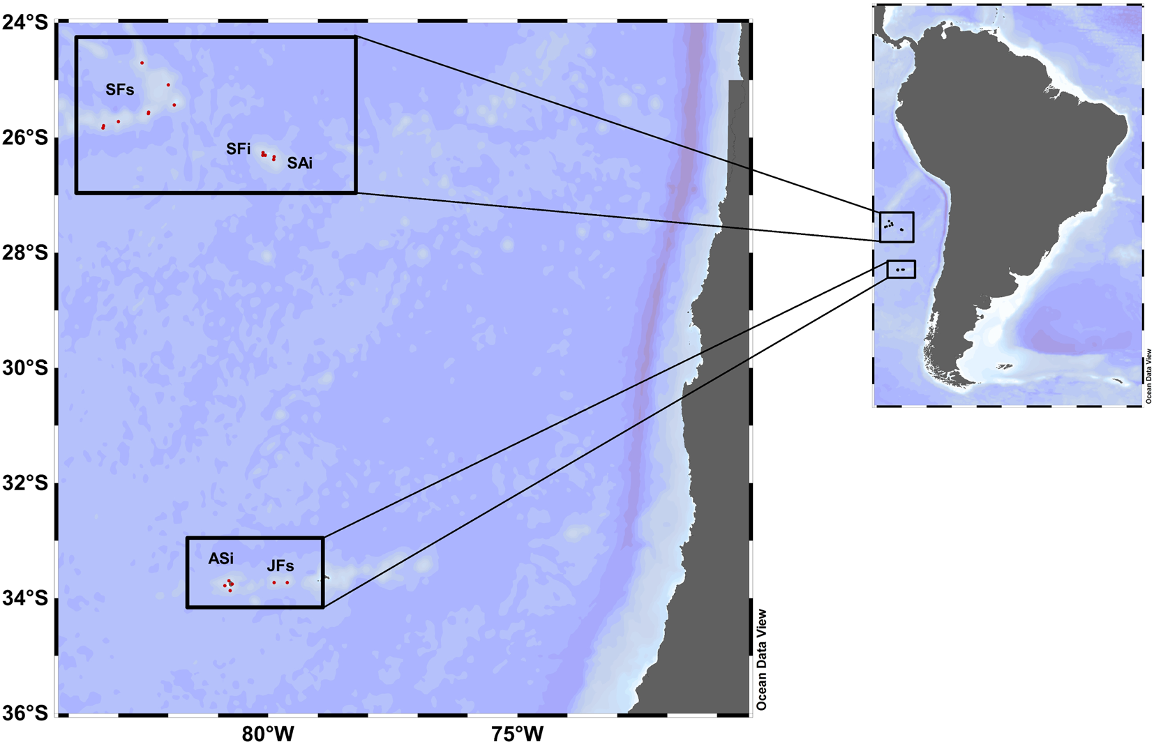
Fig. 1. Map of the South-east Pacific, illustrating the study area and showing the locations of sampling stations during the CIMAR-2 cruise in 2016. Region 1: Desventuradas archipelago: San Félix seamounts (SFs), San Félix island (SFi), San Ambrosio island (SAi). Region 2: Juan Fernández archipelago: Alejandro Selkirk island (ASi) and Juan Fernández seamounts (JFs).
Samples were preserved with 4% formaldehyde buffered with sodium borate (Smith & Richardson, Reference Silva, Rojas and Fedele1977). In the laboratory, all amphipods were sorted, counted and identified using the taxonomic keys by Bowman & Gruner (Reference Bahamonde and Castilla1973), Shih (Reference Samadi, Bottan, Macpherson, De Forges and Boisselier1991), Vinogradov et al. (Reference Vinogradov1996) and Zeidler (Reference Zeidler2004, Reference Zeidler2016). Unknown juvenile stages (<1 mm) were excluded from the analysis. The hyperiid abundance was standardized as individuals per 100 m3.
Environmental setting
During the cruise, hydrographic data were obtained at each station using a conductivity-temperature-density profiler (CTD, a SeaBird SBE-25). The CTD was deployed according to the maximum depth of each station. From these casts, vertical profiles of temperature and salinity were obtained. In addition, surface data (10 m) of the seawater's potential temperature, salinity and mixed layer depth (MLD) were obtained from the product Global ocean 1/12° physics analysis and forecast. Chlorophyll-a (Chl-a), dissolved oxygen (DO), nitrate (NO3), phosphate (PO4) and total primary production (TPP) were obtained from the product Global Ocean Biogeochemistry Hindcast. These products are part of the Copernicus Marine Environment Monitoring Service (CMEMS, http://marine.copernicus.eu/), and have a monthly temporal resolution with a spatial resolution of 0.083° and 0.25°, respectively.
Data analysis
Biological data were classified according to the sites of sampling as follows: San Félix seamounts (SFs), San Félix island (SFi), San Ambrosio island (SAi), Alejandro Selkirk island (ASi) and Juan Fernández seamounts (JFs) (Figure 1). To analyse the community structure, we first calculated total species richness (S), total individuals (NI), the diversity index of Shannon–Wiener diversity (H’) and Simpson dominance index (D) using the PRIMER-E V7 software (Anderson et al., Reference Anderson, Gorley and Clarke2008). Data were presented with mean values and their corresponding standard errors. Community descriptors were estimated as per following the equations:
 $${H}^{\prime} = - {\rm \Sigma }_{\rm i}{\rm \;}p_i{\rm \;log}\lpar {\,p_i} \rpar {\rm \;}$$
Where p i is the proportion of each i species.
 $$D\lpar {1-{\rm {\lambda }^{\prime}}} \rpar = \displaystyle{{1-\lcub {{\rm \Sigma }_i} {N_i\lpar {N_i-1} \rpar } \rcub } \over {\lcub N {\lpar {N-1} \rpar } \rcub }}$$
Where N i is the number of individuals of species i, λ’ is the probability that any two individuals from a randomly chosen sample are from the same species (representing the dominance index), whereas its complement, 1 –λ, is an equitability or evenness index (sometimes called Gini–Simpson index) (Clarke & Warwick, Reference Chiquito Vite2001). Finally, N is the total species number.
Moreover, the average taxonomic distinctness (Δ+) and variation in taxonomic distinctness (ʌ+) were calculated to show an expected average and deviation from the zone of study by comparing our data with a list of 174 species compiled from different studies conducted in the South Pacific Ocean (Vinogradov, Reference Valencia, Lavaniegos, Giraldo and Rodríguez-Rubio1991; Guillén Pozo, Reference Grice and Hart2007; González et al., Reference Gasca, Franco-Gordo, Godínez-Domínguez and Suárez-Morales2008; Gasca, Reference Gasca2009; Valencia et al., Reference Valencia and Giraldo2009, Reference Valencia, Giraldo, Valle, De Biología and De Investigación2013; Chiquito Vite, Reference Chiquito Vite2012; Gasca & Morales-Ramírez, Reference Gasca2012; Valencia & Giraldo, Reference Tranter2012; Riascos et al., Reference Raimbault and Garcia2015; Espinosa-Leal et al., Reference Espinosa-Leal and Lavaniegos2020), For this, we used the TAXDTEST routine in PRIMER-E V7 software (Anderson et al., Reference Anderson, Gorley and Clarke2008). Species were classified according to all major taxonomic levels, and the expected distribution was represented visually as a funnel plot.
Average (Δ+) and variation (ʌ+) in taxonomic distinctness were calculated by the following:
 $${\rm \Delta }^ + { = } 2\displaystyle{{\;{\rm \Sigma }{\rm \Sigma }_{i \lt jwij}} \over {N\lpar {N-1} \rpar }}$$
 $$\Lambda ^ + { = } 2\displaystyle{{\;{\rm \Sigma }{\rm \Sigma }_{i \lt j}{\lpar {{\rm \omega }_{ij}-{\rm \Delta }^ + } \rpar }^2} \over {N\lpar {N-1} \rpar }}$$
Where the double summation is taken over all species i, j; N is the species number in the sample and ωij is the assigned taxonomic path length of the branch between i and j species. ʌ + is the variance of the taxonomic distances (ωij) between each pair of species i and j, about their mean value (Δ + ) (Clarke & Warwick, Reference Chiquito Vite2001).
The hyperiid community was also examined with multivariate statistics using PRIMER7 and PERMANOVA + add-on software (Anderson et al., Reference Anderson, Gorley and Clarke2008). The species composition and abundance data (fourth-root transformed) were used to calculate the similarity matrix using the Bray–Curtis coefficient. Then, we applied a cluster and non-metric multidimensional scaling (nMDS) using the group average as a linkage technique to detect similarity. The statistical significance of the clusters was established with the SIMPROF test (Clarke & Warwick, Reference Chiquito Vite2001). The island and seamount were used as factors to test the hypothesis that the composition and abundance of the hyperiid community between these sites differed significantly.
Additionally, based on the relative abundances and frequency of species, an inverse analysis was performed following the Kaandorp technique to identify exclusive (100%), characteristic (70–99%) and generalist species (<69%) for the cluster groups (Kaandorp, Reference Hormazabal, Shaffer and Leth1986). The correlation between the hyperiid community and environmental conditions was assessed using surface values (10 m) of oceanographic variables from the closest pixel to the location of the sampling station with the distance-based linear model (DistLM). The method used was the specific selection from an R2 criterion. The best solution was found using the stepwise selection as per the AICc R2 criterion. A distance-based redundancy analysis (dbRDA) by stations was used to visualize the observed relationships (Primer-E Version 7).
Results
Oceanographic conditions
Warmer and saltier conditions prevailed in the Desventuradas region (mean of temperature = 17.58°C, mean salinity = 34.89) (Figure 2A) compared with the Juan Fernández region (mean temperature = 15.06°C and mean salinity = 34.22) (Figure 2B). Subtropical waters (STW) prevailed in the upper layer of Desventuradas, while subantarctic water (SAAW) appeared to dominate in near-surface layers of Juan Fernández. The in situ data are in agreement with the monthly mean values of surface data shown in Figure 2C in which San Félix seamounts (SFs), San Félix island (SFi) and San Ambrosio island (SAi) have warmer (~18–19°C) and more saline (~35) conditions than Alejandro Selkirk island (ASi) and Juan Fernández seamounts (JFs) (~17.0°C and ~34.00, respectively).

Fig. 2. Vertical profiles of temperature (T) and salinity (S) by stations during CIMAR-22 cruise for (A) Desventuradas region and (B) Juan Fernández region. (C) Monthly means at superficial depth (10 m) of potential temperature (ST) and salinity (SS) in the study area. Data are mean values of October and November of 2016. Black dots show the sampling stations.
Monthly means show a deeper MLD in SFs, SFi and SAi (~20–23 m except in SFs_8 = 17 m) than in ASi and JFs (~13–16 m) (Figure 3). In addition, DO showed similar values at all stations (values > 230 mmol m−3) with highest values in ASi (all stations) and JF_10 with ~252 mmol m−3 and ~251 mmol m−3, respectively. The lowest values were found to be in SFs, SFi and SAi (~234–240 mmol m−3) (Figure 3).

Fig. 3. Monthly means of surface data of the mixed layer depth (MLD), dissolved oxygen (DO), chlorophyll-a (Chl-a), total primary production (PP), nitrate (NO3) and phosphate (PO4). Data are mean values of October and November of 2016. Black dots show the sampling stations.
Regarding nutrient concentrations, the highest estimates for the Desventuradas region were found in SFs_2 (NO3 = 0.36 mmol m−3 and PO4 = 0.45 mmol m−3). Meanwhile, in the Juan Fernández region, the highest values were found in ASi_292 (NO3 = 2.43 mmol m−3 and PO4 = 0.36 mmol m−3) and JFs_11(NO3 = 2.64 mmol m−3 and PO4 = 0.44 mmol m−3) (Figure 3).
The entire study area exhibited oligotrophic conditions. For instance, in the Desventuradas region, surface Chl-a was ~0.04 mg m−3 in most SFs (except SFs_3 and SFs_2 with 0.09 and 0.14 mg m−3, respectively), but values of 0.20 mg m−3 were found in SFi. In the case of Juan Fernández, surface Chl-a ranged between 0.19 and 0.23 mg m−3 for ASi, and 0.14–0.17 mg m−3 for JFs.
TPP was slightly high in the islands with values of 6.88 mg C m−3 day−1 in SFi and 9.39 mg C m−3 day−1 in ASi. In contrast, lower values were observed for SFs (0.11–0.13 mg C m−3 day−1, except SFs_3 = 1.58 mg C m−3 d−1 and SFs_2 = 3.42 mg C m−3 day−1) and JFs_10 with 5.05 mg C m−3 day−1 and JFs_11 with 0.14 mg C m−3 day−1(Figure 3).
The hyperiid community
A total of 56 species of hyperiids (infraorder: Physocephalata) were identified as belonging to 15 families and 29 genera (Table 1). The analysis of community descriptors did not show significant differences between the sites (Kruskal–Wallis test, P > 0.05). In the islands, the highest values of species richness (S), Shannon–Wiener diversity (H’) and dominance (D) were found in SAi (31, 2.84 and 0.92, respectively), but the higher total number of individuals (N) was found in ASi. In the seamounts, all highest values were found in SFs (S = 38, N = 357, H’ = 2.80 and D = 0.90) (Figure 4A).

Fig. 4. (A) Mean and standard error of species richness (S), total individuals (N), Shannon–Wiener diversity (H’) and Simpson dominance (D). (B) Average taxonomic distinctness (Δ+) and variation in taxonomic distinctness (ʌ+) for the hyperiid community in the study area. The central line shows mean values and the continuous lines are the distribution of probability at 95%.
Table 1. Total abundance (ind. 100 m−3) of hyperiid amphipod species found in the study area

Number of stations (N) where the species were found from a total of 19 stations and relative abundance (%). The data are grouped according to the sites of sampling as: San Félix island (SFi), San Ambrosio island (SAi), Alejandro Selkirk island (ASi), Juan Fernández seamounts (JFs) and San Félix seamounts (SFs).
Variation in average taxonomic distinctness (delta + ) is shown in Figure 4B. The hyperiid community richness found in our study was lower than the expected mean for the whole region. Particularly, stations SFi_18 and SFs_6 were found outside the limits of confidence (95%), showing lower diversity than the expected value (0.6% and 2.6% of significance). In contrast, the average taxonomic variation (lambda + ) (Figure 4C) showed that most stations were near the average of the confidence interval, except for stations ASi_29 and SFi_18 with an 11.4% significance in both cases.
The total hyperiid abundance found in the islands was 771.59 ind. 100 m−3 where the highest values were found in ASi with 391.75 ind. 100 m−3, while in seamounts the total observed abundance decreased to about half of that (471 ind. 100 m−3) with the highest values in SFs (357.47 ind. 100 m−3). Considering sites, the most abundant species (adding up to >50% of total abundance) were similar in all cases: for Desventuradas, in SFi, the 52% was represented by Eupronoe minuta Claus, 1879, Eupronoe laticarpa Stephensen, 1925, Primno latreillei Stebbing, 1888, Lestrigonus schizogeneios and Hyperietta vosseleri Stebbing, 1904. In contrast, 54% of SAi was represented by Primno latreillei, Phrosina semilunata, Primno brevidens Bowman, 1978, Hyperioides longipes and L. schizogeneios. Finally, the most abundant (51%) species in SFs were P. latreillei, P. semilunata, H. longipes and E. minuta (Figure 5A, Table 1). In the case of Juan Fernández, in ASi, only P. semilunata and L. schizogeneios represented 55% of total abundance, and in JFs, the most abundant species (54%) were the same as that of ASi, i.e. L. schizogeneios and P. semilunata (Figure 5B, Table 1).

Classification and ordination analyses, based on the abundances of all species yielded three clusters, suggesting differences among regions in the study area. Cluster 1 showed an average similarity of 50.76% and grouped all stations of Desventuradas islands, Cluster 2 showed a similarity of 52.06% and Cluster 3 showed a similarity of 34.62% (Figure 6). The results of the inverse analysis (Supplementary Figure S1) for the clusters suggested that most species fall in the category of generalist (28 species) in which Vibilia armata Bovallius, 1887, Hyperietta stephenseni, Phronimella elongata Claus, 1862, Paraphronima Gracilis Claus, 1879 and Tryphana malmii Boeck, 1871 were present in all clusters with a frequency of occurrence (FO) >25% in most cases. In contrast, the category of characteristic species varied between clusters with Simorhynchotus antennarius Claus, 1871, L. schizogeneios, P. semilunata, Brachyscelus rapax Claus, 1879, Amphithyrus bispinosus Claus, 1879, Lestrigonus shoemakeri Bowman, 1973, and Themistella fusca Dana, 1853 in Cluster 1, Streetsia challengeri in Cluster 2 and P. latreillei and Anchylomera blossevillei Milne-Edwards, 1830 in Cluster 3. Finally, exclusive species with the lowest abundance and FO were found in Clusters 1 and 3.

Fig. 6. Cluster analysis based on the Bray–Curtis similarity matrix among stations. The dendrogram shows the significant differences among clusters (black lines) using the simprof test (P < 0.05).
Considering the whole community, we found that the species most important in this study were P. semilunata with an FO of 94.44%, L. schizogeneios and H. stephenseni with an FO of 88.89% and H. longipes, P. elongata and P. latreillei with an FO of 72.22%.
Environmental correlates
When examining the influence of environmental variables on the hyperiid community structure in terms of composition and abundance, the DistLM analysis detected significant associations with all tested variables, except for PO4 (Supplementary Table S2A). Environmental variables explained as much as 46.51% of variation with an individual contribution of surface temperature (12.37%), salinity (10.46%), DO (6.44%), MLD (5.13%), Chl-a (3.35%), PP (4.70%), PO4 (1.40%) and NO3 (2.62%) (Supplementary Table S2B). Considering the best solution model using the stepwise selection, salinity was selected (AIC = 141.45, R2 = 0.196). The first two dbRDA axes reflected a 61.64% variation in the fitted model and 28.67% of the total variation. The first axis was negative in relation to SS, ST and MLD and positive with NO3. The second axis showed a strong negative relationship with DO (Figure 7).

Fig. 7. Distance-based redundancy analysis (dbRDA) of the selected environmental variables that best explain the variation of the hyperiid abundance across the study area. The dbRDA was performed using the best-fit explanatory variables obtained from a multivariate multiple regression analysis (the DistLM results can be found in Table S2).
Discussion
The hyperiid community from the seamount regions
Given the hydrographic variability and locations of both regions, we expected a heterogeneous composition and distribution of hyperiids. However, except for a small group of rare species (low frequency and abundance) that were found exclusively in Juan Fernández (e.g. Pronoe capito, Paralycaea gracilis and Brachyscelus crusculum Bate, 1861), the composition of species was similar in both archipelagos. Shared species between the two regions of islands and seamounts have been reported for fishes, suggesting the two regions should be considered as a single biogeographic unit, within which the local fauna is closely related to the Indo-West Pacific biogeographic province rather than the Eastern Pacific province (Parin et al., Reference Palma and Silva1997; Pequeño & Sáez, Reference Parin, Mironov and Nesis2000; Dyer & Westneat, Reference Doty and Oguri2010). Locally, the species found in our study had been previously reported in other areas of Chilean waters (Meruane, Reference Lavelle and Mohn1980, Reference Meruane1982; Espinosa-Leal et al., Reference Espinosa-Leal and Lavaniegos2020), but in most cases, the abundance is highest in the islands and seamounts compared with the coastal upwelling zone. Furthermore, the presence of the same species in the coastal upwelling region and the island and seamounts provides evidence of the ecological connectivity of the regions, either from dispersal or by advection of species between sites. In this context, other works have suggested limited connectivity or the presence of some oceanographic barriers to prevent a common fauna or allowing low gene flow between the two regions (Aniñir Velásquez, Reference Andrade, Sangrà, Hormazabal and Correa-Ramirez2019; González et al., Reference González, Haye, Balanda and Thiel2020), therefore supporting the view of the high-level of endemism in these zones. This limited connectivity was observed in the North Pacific for the hyperiid Themisto, in which the species may have a different population origin (Tempestini et al., Reference Stramma, Bange, Czeschel, Lorenzo and Frank2017). In fact, the difficulty to distinguish the local endemicity from sampling biases arising from the occasional collection of widespread species (Clark et al., Reference Clarke and Warwick2010) highlights the importance of combining the taxonomic analysis with other approaches (e.g. genetic markers or other molecular methods) to study the communities in these isolated places. The correlation between environmental variables and the amphipod community was similar to that observed in other regions, with different water mass composition and hydrographic conditions. For instance, surface salinity was the best predictor of the amphipod community structure in the Gulf of California (Siegel-Causey, Reference Shulenberger1982), Northern Queensland (Zeidler, Reference Yáñez, Silva, Vega, Espíndola, Álvarez, Silva, Palma, Salinas, Menschel, Häussermann, Soto and Ramírez1984) and the Panama Bight (Valencia et al., Reference Valencia, Giraldo, Valle, De Biología and De Investigación2013). In the eastern Indian Ocean, P. elongata, A. blossevillei and H. stephenseni were associated with lower temperature and higher salinity of the subtropical water mass (Tranter, Reference Tolosa, Miquel, Gasser, Raimbault, Azouzi and Claustre1977). Furthermore, the analysis of salinity and temperature associated with thermohaline circulation contributed to the classification of the species L. schizogeneios as eurythermal and euryhaline (Zhaoli, Reference Zeidler2009), and this assignation may explain why this is one of the most abundant species in the study. In any case, the strong link between some abundant species and salinity and temperature provides evidence that the spatial distribution of water masses and their properties may control the distribution and composition of the hyperiid community.
Biogeographic characteristics
This work should be considered as the first survey of the hyperiid amphipod community in the Desventuradas archipelago and, thus, complements the information on this group to that of Yáñez et al. (Reference Weil, Duguid and Juanes2009) for Juan Fernández archipelago and that of Vinogradov (Reference Valencia, Lavaniegos, Giraldo and Rodríguez-Rubio1991) for the Nazca and Salas y Gómez ridge. In general, the hyperiid species found in our study are widely distributed in the world oceans, and they have a tropical and subtropical distribution (Vinogradov et al., Reference Vinogradov1996; Zeidler, Reference Zeidler2004). This pattern is the same for the biogeographic origin of benthic communities in the same zone (Friedlander et al., Reference Frederick, Escribano, Morales, Hormazabal and Medellín-Mora2016). Regarding the taxonomic composition of the hyperiid community, a total number of 56 species were found. This number is lower than that of larger-scale studies (Vinogradov, Reference Valencia, Lavaniegos, Giraldo and Rodríguez-Rubio1991; Burridge et al., Reference Bowman and Gruner2016; Espinosa-Leal et al., Reference Espinosa-Leal and Lavaniegos2020), but it is greater than those found in similar ecosystems, such as in Brazil (Souza et al., Reference Smith and Richardson2016), the Eastern Tropical Pacific (Gasca & Morales-Ramírez, Reference Gasca2012; Valencia & Giraldo, Reference Tranter2012) and the Caribbean Sea (Gasca & Shih, Reference Gasca and Morales-Ramírez2003). Differences may arise from variable sampling techniques and gears, variable sampling seasons, and possibly distinct diversity patterns. For our study region, a close comparison could be possible with the previous work of Vinogradov (Reference Valencia, Lavaniegos, Giraldo and Rodríguez-Rubio1991) in the South Pacific gyre (SPG) across the ridges of Nazca and Salas y Gómez, which shows that the species Pronoe capito, Paralycaea gracilis (Claus, 1879), Brachyscelus rapax, Glossocephalus milneedwardsi, Tetrathyrus forcipatus (Claus, 1879), Phronima dunbari (Shih, 1991), and Primno macropa had not been previously reported. Moreover, the most abundant species, except for Phrosina semilunata (the first rank in our study) were different, such as Phronima atlantica (first rank in the SPG) in our study only represented a 0.91% of total abundance; Phronimella elongata (4.11%), Anchylomera blossevillei (2.50%) and Primno brevidens (2.42%), which were ranked between 7th and 10th, whereas in the SPG, this species was ranked in the 2nd, 3rd and 5th place in terms of abundance. In contrast, Lestrigonus schizogeneios and Primo latreillei (our 2nd and 3th rank) were considered scarce in the SPG. The absence of other hyperiid species in our study belonging to the Physosomata infraorder has probably resulted from differences in sampled depth strata. Samples from deeper layers should increase the biodiversity inventory of this group, especially by adding species inhabiting the mesopelagic realm. With respect to other oligotrophic systems, Lestrigonus schizogeneios, Hyperioides longipes and Phrosina semilunata have been the most common species found in the Sargasso Sea (Grice & Hart, Reference González, Goetze, Escribano, Ulloa and Victoriano1962; Gasca, Reference Friedlander, Ballesteros, Caselle and Gaymer2007), whereas Primno latreillei is the most abundant species in the North Pacific Gyre (Shulenberger, Reference Shih1977). Finally, as compared with studies in other islands, differences in the hyperiid composition (especially the most common and abundant species) became evident, indicating that despite the fact that most hyperiids have a widespread distribution, each region has a distinct local fauna and associated with local hydrographic conditions.
Oceanographic drivers
Although both seamount regions are located in the oceanic and oligotrophic waters of the SEP (Pizarro et al., Reference Petrillo, Giallain and Della Croce2006), the Juan Fernández archipelago may be under a greater influence of the coastal upwelling zone, thus showing the biological and physical characteristics of the Coastal Transition Zone (CTZ) (Hormazabal et al., Reference Guillén Pozo2004), whereas Desventuradas may mostly exhibit offshore conditions. The in situ and monthly mean data of sea surface temperature and salinity are in agreement with other studies that show the surface predominance of subtropical water (STW) in Desventuradas, while in Juan Fernández, subantarctic water (SAAW) prevails (Bahamonde, Reference Aniñir Velásquez1987; Moraga & Argandoña, Reference Meruane2001; Silva et al., Reference Siegel-Causey2009; Aniñir Velásquez, Reference Andrade, Sangrà, Hormazabal and Correa-Ramirez2019). It is important to add the possible presence of equatorial subsurface water (ESSW) below 200 m, as found in other studies (Yáñez et al., Reference Weil, Duguid and Juanes2009; Frederick et al., Reference Fordham and Brook2018; Fierro, Reference Fernández and Hormazábal2019), but that could not be corroborated in our study due to limited CTD data from deep water.
Although in the oceanic waters surrounding the archipelagos, some patches of Chl-a (~0.25–1 mg m−3) can be found, representing the coastal transition zone (Morales et al., Reference Moraga and Argandoña2010), the slight increases in Chl-a and PP near the islands, as compared with seamount zones, may be associated with greater phytoplankton biomass resulting from the island mass effect (IME) (Doty & Oguri, Reference Dirnböck, Greimler, Lopez and Stuessy1956; Andrade et al., Reference Andrade, Hormazabal and Correa-Ramirez2014a, Reference Andrade, Hormazábal and Correa-Ramírez2014b). These increases in phytoplankton biomass (between 0.07 and 0.30 mg m−3) agree with previous studies in Desventuradas, Alejandro Selkirk island (Pizarro et al., Reference Petrillo, Giallain and Della Croce2006) and the Juan Fernández archipelago (Andrade et al., Reference Andrade, Sangrà, Hormazabal and Correa-Ramirez2012). The predominance of pico- and nanophytoplankton may explain the increased biomass of phytoplankton (Tolosa et al., Reference Tempestini, Fortier, Pinchuk and Dufresne2007; Von Dassow & Collado-Fabbri, Reference Vinogradov, Volkov, Semenova and Siegel-Causey2014), which, in this area, can have a direct relationship with Chl-a, PP and nutrients.
The low values of nitrate (0.36–2.64 mmol m−3) and phosphate (0.15–0.45 mmol m−3) were similar to those found in previous studies, such as in the CIMAR 5 cruise (Von Dassow & Collado-Fabbri, Reference Vinogradov, Volkov, Semenova and Siegel-Causey2014). Off-shore water is well known for having N and P deficiencies in the SEP (Raimbault & Garcia, Reference Pizarro, Montecino, Astoreca, Alarcón, Yuras and Guzmán2008; Farías et al., Reference Espinosa-Leal, Escribano, Riquelme-Bugueño and Corredor-Acosta2013; Stramma et al., Reference Souza, Conceição, Oliveira and Junior2013; Cornejo D'Ottone et al., Reference Clark, Rowden, Schlacher, Williams, Consalvey, Stocks, Rogers, O'Hara, White, Shank and Hall-Spencer2016; Wang et al., Reference Von Dassow and Collado-Fabbri2019).
Conclusion
Despite the described differences in oceanographic conditions in these two apparently isolated seamount regions, oceanographic processes, such as large-scale circulation and mesoscale activity, appear to be major mechanisms that promote connectivity between the regions along with the coastal upwelling system, thereby integrally forming a unique and single biogeographic unit for hyperiid amphipods.
Supplementary material
The supplementary material for this article can be found at https://doi.org/10.1017/S0025315420001344
Acknowledgements
We are grateful to Daniel Toledo and Leissing Frederick for assisting with the zooplankton sampling and the crew of ‘Cabo de Hornos’ for providing additional valuable technical assistance. This work is a contribution for the international networking project Integrated Marine Biosphere Research (IMBeR) and the TROPHONET project REDES 10039. We would also like to thank the two anonymous reviewers, whose comments and corrections greatly improved an earlier version of the work.
Financial support
The CIMAR-22 cruise and this work were funded by the Comité Oceanográfico Nacional (CONA) of Chile. Additional financial support was provided by the Millennium Institute of Oceanography (Grant ICN12_019) and FONDECYT project 118-1682.


