FARM PRODUCTIVITY DATA

The long-run path of U.S. agricultural inputs, outputs, innovations, and productivity has been the subject of a rich literature, including works by Cochrane (Reference Cochrane1958, 1993), Olmstead and Rhode (Reference Olmstead, Rhode, Stanley and Robert2000, 2001, 2002, 2006a, 2006b, 2008), Gardner (2002), Dimitri, Effland, and Conklin (2005), and a host of others cited and discussed by Alston et al. (Reference Alston, Andersen, James and Pardey2010).Footnote ³ Building on this foundation, we use newly created measures in longer-run series to quantify and interpret the evolving path of aggregate U.S. farm inputs, outputs, and productivity over most of the twentieth century and into the early twenty-first century.

Measuring productivity is a difficult task; detecting and interpreting changes in productivity growth rates can be even more difficult. The measures used matter. We developed a range of productivity measures for the U.S. farm economy, stretching back a century or so.Footnote ⁴ The InSTePP Production Accounts (version 5) consist of detailed state-specific data on inputs and outputs in U.S. agriculture for the period 1949–2007. Using these data we constructed Fisher ideal approximations to Divisia indexes of aggregate quantities of inputs and outputs for the farm sector in each of the 48 contiguous U.S. states, various multistate regions, and the United States as a whole. The highly disaggregated base data permitted the construction of indexes with adjustments for heterogeneity within major categories of inputs (e.g., age and horsepower of tractors in the capital stock or age and education of farm operators in the labor input) and outputs at the state and national levels. These quality-adjusted state-specific indexes can be used to analyze national, regional, and state-specific trends in multifactor productivity (MFP) and in several partial factor productivity (PFP) measures for the period 1949–2007.Footnote ⁵

Initial work with an earlier version of these data (e.g., Alston et al. Reference Alston, Andersen, James and Pardey2010) provided evidence of a slowdown in productivity growth since 1990, but also raised some questions that require consideration of the prior history for which such detailed data on inputs, outputs, and productivity are not available. Hence, to place the post-WWII evidence in a longer-run setting, we backcast the InSTePP measures of national agricultural productivity to 1910, using year-on-year changes in the commensurate measures of MFP and quantities of land and labor compiled by the USDA.Footnote ⁶ In a companion study to the present work, Andersen et al. (Reference Andersen, Alston, Pardey and Aaron2018) applied a battery of measures to the resulting long-run MFP data, as well as various PFP measures (such as labor productivity, land productivity, and yields per acre for various crops), to test for longer-term changes in productivity growth. These analyses, as well as analyses using the more-detailed data after 1948, consistently reveal a phenomenon of accelerating growth peaking in the 1960s or 1970s, followed by a progressive slowdown, visibly apparent in plots of the data and statistically significant after 1980. In this framework, the recent slowdown can be seen as a return to a more-normal long-run average growth rate, following a period of abnormally high rates in the period of the 1950s through the 1980s.

These findings are new and controversial. They conclude and largely settle our longstanding debate with USDA economists—see, for example, Ball, Wang, and Nehring (2010), Wang (Reference Wang2010), Ball, Schimmelpfenning, and Wang (2013), and Wang et al. (Reference Wang, Paul, David and Eldon2015a, 2015b)—who maintained that U.S. farm productivity growth had not slowed since the 1950s. The present work arose in part from that debate. Here, using different procedures and some different data, we report new results that extend and reinforce the results from Andersen et al. (Reference Andersen, Alston, Pardey and Aaron2018). We place these U.S. farm productivity patterns in the context of the changing structure of agriculture and the corresponding productivity patterns in the broader national economy, setting the scene for our deeper analysis of the main drivers of the farm productivity surge and slowdown.

U.S. FARM PRODUCTIVITY, 1910–2007

Our analysis begins with the most comprehensive but also most aggregative measure: data on national agricultural MFP over the longer period, 1910–2007. We describe the patterns in the data and the results from tests for a slowdown, constant growth, or a surge.Footnote ⁷

Over the course of the century, the index of the aggregate quantity of output (Q) from U.S. agriculture grew from 100 in 1910 to 463 in 2007, at a rate of 1.58 percent per year.Footnote ⁸ Meanwhile, the index of the aggregate quantity of inputs (X) used in U.S. agriculture grew by just 0.16 percent per year, reflecting some increases in capital and materials inputs that offset the reductions in the use of land (after the late 1970s) and especially labor. Consequently, the measure of MFP (MFP = Q/X) grew at a rate of 1.42 percent per year (Figure 1). The implication is that U.S. agriculture produced 4.6 times as much aggregate output in 2007 as in 1910 without appreciably increasing the quantity of aggregate input.

Figure 1 QUANTITY INDEXES OF OUTPUT, INPUT, AND MFP, U.S. AGRICULTURE, 1910–2007

Notes: All of the series refer to the left axis except for land per farm (right axis). The sudden decline in land in farms in 1993 reflects a change in the definition of farms (USDA-NASS 1999, p. 13) that had the measured number of farms increasing by 4.5 percent from 1992 to 1993. We omitted the 2007 estimate as USDA-NASS (2014a, p. 21) reported a sudden increase in the reported number of farms (by 5.3 percent from 2006 to 2007) attributed to “…methodological changes that allowed NASS to more accurately count small farms in the 2007 census” with a commensurate large drop in the average acres per farm from 443 in 2006 to 418 in 2007.

Sources: Index numbers were calculated by the authors using the InSTePP Production Accounts, version 5 augmented with data from USDA-ERS (1983). Number of farms and land in farms are from Olmstead and Rhode (2006a, series D19 and D6 series) for 1910 to 1997 and from USDA-NASS (2019) for 1998 to 2007.

The long-run path was not always smooth. Year-to-year variations in aggregate output (and to a much lesser extent measured aggregate input use) make it difficult to discern the onset, magnitude, and duration of a productivity slowdown.Footnote ⁹ To test for secular changes in productivity growth usually entails comparing longer sub-periods in which some of the year-to-year variation is smoothed out—for instance, the data are summarized by decade in Table 1, which shows period-specific growth rates in U.S. aggregate agricultural input, output, and MFP as well as measures of land and labor productivity. As shown in Table 1, our measures of MFP and PFP growth have varied considerably from decade to decade, with relatively high rates of growth during the period 1950–1980, when the rate of growth of aggregate output was also relatively high, and relatively slow rates of growth since then.Footnote ¹⁰

Table 1 ANNUAL AVERAGE GROWTH RATES IN U.S. AGRICULTURAL OUTPUT, MFP, AND LABOR AND LAND PFP, AND IN AGRICULTURAL R&D SPENDING AND STOCKS 1910–2007

Notes: All figures are annual average growth rates for the respective periods calculated by the log-difference method.

¹ Data on trapezoidal-lag knowledge stocks are available from 1925. Thus, for the periods 1920–1930, 1910–1950, and 1910–2007, growth rates are for 1925–1930, 1925–1950, and 1925–2007, respectively.

² Data are gamma-lag knowledge stocks available from 1939. Thus, for the periods 1910–1950 and 1910–2007, growth rates are for 1939–1950 and 1939–2007 respectively.

Sources: Growth rates of productivity indexes were calculated by the authors using the InSTePP Production Accounts, version 5, augmented with data from USDA-ERS (1983). Growth rates of R&D spending and knowledge stocks were calculated by the authors using the InSTePP public agricultural R&D series for the United States.

Using essentially the same data, Andersen et al. (Reference Andersen, Alston, Pardey and Aaron2018) estimated logarithmic segmented trend models and polynomial trend models in which the linear logarithmic model, representing constant exponential growth, is a nested special case. The hypothesis of the linear logarithmic model with a constant growth rate is strongly rejected, and their results (see also Online Appendix B) support the view that U.S. farm productivity growth has slowed in recent decades. But more than that, they also suggest that this slowdown came after a period of unusually rapid productivity growth. Multifactor productivity grew by 1.42 percent per year for 1910–2007, but this long-term average reflected a period of below-average growth at 0.83 percent per year for 1910–1950, above-average growth at 2.12 percent per year for 1950–1990, and again below-average growth at 1.16 percent per year for 1990–2007. State-specific data confirm these findings.Footnote ¹¹

Partial factor productivity measures reinforce the evidence from the multifactor productivity measures. Over the period 1910–2007, compared with MFP, the PFP of land grew more slowly, averaging 1.38 percent per year while the PFP of labor grew relatively rapidly, averaging 2.90 percent per year, as the labor intensity of farming was falling substantially (e.g., Alston et al. Reference Alston, Andersen, James and Pardey2010, figure 3-14). U.S. agricultural land was 3.8 times more productive in 2007 than it was in 1910, and labor was 16.7 times more productive, reflecting the great exodus of farmers and other farm labor—even after appropriate adjustment for the partially offsetting improvements to land (mainly irrigation) and the enhanced educational status and work experience (increased age) of farm operators. Analysis of U.S. national average crop yields for barley, corn, oats, rice soybeans, and wheat back to the mid-nineteenth century indicates that the 1950s, 1960s, 1970s, and 1980s were decades of abnormally high rates of yield growth.Footnote ¹²

AGRICULTURAL MFP IN A NATIONAL MFP CONTEXT

The shifting sands of U.S. agricultural productivity growth were part and parcel of similar shifts in productivity growth in the broader economy. The long-run productivity performance of the U.S. economy has received considerable attention from economists, especially in the context of periodic concerns over slowdowns in economic growth, and the broad consensus is that national MFP growth slowed considerably since the 1960s after a mid-century surge.Footnote ¹³ Comparatively little attention has been paid to the long-run productivity performance of the agricultural sector as an element of and compared with the economy as a whole. Of specific interest here is the linkage between the surge and slowdown in national MFP growth and the surge and slowdown we have identified in U.S. agricultural MFP growth.

A mechanistic relationship among sectors of the economy is implied by the arithmetic of productivity measures. Specifically, the growth rate of U.S. private business MFP (\[{g_U}\]) is a weighted average of the farm and non-farm MFP growth rates (\[{g_F}\] and \[{g_N}\], respectively), where the weights are sector shares of the total quantity of inputs.Footnote ¹⁴ That is:

\\[{{\text{g}}_{\text{U}}} = {s_F}{{\text{g}}_{\text{F}}} + (1 - {s_F}){{\text{g}}_{\text{N}}}.\]

Rearranging terms, the growth rate of U.S. private business MFP is equal to the growth rate of farm MFP plus the difference between the farm and non-farm MFP growth rates weighted by the non-farm share of aggregate inputs:

\[{{\text{g}}_{\text{U}}} = {{\text{g}}_{\text{F}}} + (1 - {s_F})({{\text{g}}_{\text{N}}} - {{\text{g}}_{\text{F}}}).\]

These equations illustrate the direct connections between growth in productivity of the farm sector and the broader (farm and non-farm) national economy. Less-direct connections reflect technology spillovers and factor movements. As noted by Kuznets (Reference Kuznets1961, p. 69) “if agriculture grows it makes a product contribution; if it trades with others it renders a market contribution; if it transfers resources to other sectors, these resources being productive factors, it makes a factor contribution” (emphasis in original). During the first half of the twentieth century, relatively rapid growth of the non-farm sector came partly at the expense of the farm sector—especially by attracting labor away from farms (Kendrick and Jones 1951)—with implications both for labor-saving innovations on farms and the growth rate of farm productivity as well as for the farm share of the total economy. In the early 1900s, agriculture accounted for one-third of the national economy: rural-urban migration mattered, and changes in agricultural productivity had meaningful impacts on national productivity measures.Footnote ¹⁵ By the early 2000s, agriculture’s share of the economy had shrunk to the extent that changes in agriculture had little consequence for economy-wide measures of economic performance.

These connections are reflected in the measures of U.S. farm, nonfarm, and aggregate (farm and non-farm) private business MFP growth reported in Table 2. The long-term aggregate and non-farm MFP series were created by splicing indexes from Kendrick (1961, 1973) to create annual indexes for 1899–1947, which, in turn, were used to backcast the corresponding series from BLS (2020) for 1948–2018. We include two measures of MFP growth for the farm sector. The first is the InSTePPUSDA series for 1910–2007, as depicted in Figure 1, which was created by using the historical USDA series to backcast the 1949–2007 InSTePP series from 1949 to 1910. The second (InSTePP-Kendrick) uses indexes from Kendrick (1961, 1973) instead of the USDA to backcast the 1949–2007 InSTePP series from 1949 to 1890. The InSTePP-USDA series is preferred, but the latter is included because it is a longer series and directly comparable to the other (national and non-farm sector) series based on Kendrick for the years prior to 1948.

Several points may be drawn from Table 2. In the 1890s, overall private business MFP grew by 1.14 percent per year reflecting a slightly faster rate of growth in the farm sector, 1.27 percent per year, combined with a slower rate in the non-farm sector, 1.08 percent per year. Over the next two decades, however, negligible productivity growth in the farm sector—still a significant share of the economy—held the national aggregate MFP growth rate well below that for the non-farm sector. The long-term (1910–2007) annual average MFP growth rate for the farm sector was 1.42 percent per year, a little less than the aggregate private business sector rate of 1.54 percent per year. However, during the period 1910–1950, in the non-farm sector, MFP grew by 1.93 percent per year on average, more than twice the rate for the farm sector, 0.83 percent per year. For the subsequent period, 1950–2007, these roles were reversed: MFP grew by 1.83 percent per year in the farm sector but just 1.13 percent per year in the non-farm sector.

In Table 2, U.S. non-farm productivity growth accelerated in the 1910s and 1920s, peaking in the 1930s and 1940s, and began to slow appreciably in the 1950s, with a sharp drop in the 1970s. Hence, for the non-farm sector, annual average MFP growth rates exceeded the long-term (1910–2007) average for the decades of the 1910s through the 1940s and for the 1960s, and they have been below the long-term average from the 1970s on. Farm productivity followed a similar pattern, but two decades later, with above-average productivity growth rates for the decades of the 1930s through the 1980s. Combining these two elements, and noting the further decline of the farm share of the total economy, helps account for the surge in aggregate MFP growth during the decades of the 1920s through the 1960s. Farm productivity growth rates remained high into the 1970s and 1980s, well above their non-farm sector counterparts, but by then the farm share of the economy had shrunk to just a few percent—too little to be of much consequence in sustaining the national productivity growth rate.

Table 2 ANNUAL AVERAGE U.S. FARM, NON-FARM AND TOTAL PRIVATE BUSINESS MFP GROWTH RATES, 1890–2007

Notes: Shading indicates the decades with growth rates above the long-term (1910–2007) average. MFP growth rates of the respective periods calculated by the log-difference method. Labor includes the number of full-time equivalent employees plus the number of self-employed persons and unpaid family workers.

Sources: Growth rates of productivity indexes were calculated by the authors using the InSTePP Production Accounts, version 5 (1949–2007), augmented with data from USDA-ERS (1983) or Kendrick (1961, 1973) and BLS (2020). Labor data were calculated by the authors using data on persons engaged in production from BEA (2020a), on unpaid family workers from Carter and Sutch (Reference Sutch2006) and Sutch (Reference Sutch2006), and on engaged persons from Kendrick (1961). Agricultural GDP as a share of GDP is authors’ calculations based on GDP data from Johnston and Williamson (Reference Johnston and Williamson2020), and AgGDP data from the United Nations (2020), BEA (2020b), and U.S. Bureau of Census (1949).

These informal impressions are confirmed by fitting a cubic polynomial trend model in logarithms to each of the data series summarized in Table 2 for the period 1910–2007. In each case the model fits the data fairly well (R2 values of at least 0.98) and we can strongly reject the nested special case of a linear model with a constant exponential growth rate against the alternative of a cubic model that implies a surge and a slowdown.

At the start of the twentieth century, agriculture accounted for one-sixth of U.S. GDP, while employing a much larger share of the national labor force—more than one-third. Over the course of the twentieth century the rest of the economy grew much faster, and agriculture’s share of GDP shrank by a factor of 15: from 15 percent in 1900–1910 to 1 percent in 2000–2007. Agriculture’s contribution to GDP grew in real terms, although its share was shrinking. The farm sector share of the total labor force fell too, by a greater proportion, a factor of 24: from 34 percent in 1900–1910 to 1.4 percent in 2000–2007. Total private employment of labor increased fourfold, while employment of labor on farms shrank sixfold. Some of the associated movement of labor and resulting convergence in wage rates across sectors (e.g., Gardner 2002) entailed significant interregional movement of people (e.g., Caselli and Coleman 2001).

In what follows, we develop and discuss a range of evidence related to potential drivers of the twentieth century surge and slowdown in U.S. farm productivity. In the next three sections, respectively, we compare the timing of the surge and slowdown in productivity with the time path of research-related knowledge stocks, the time path of uptake for different classes of on-farm innovation, and the timing of the structural transformation of the national farm economy. Finally, we briefly consider the potential effects of exogenous changes in the physical and regulatory environment that might have constrained agricultural productivity directly or done so indirectly by restricting the use of some technologies.

AGRICULTURAL R&D AND KNOWLEDGE STOCKS

Over the course of the twentieth century, following the closing of the physical frontier, American agricultural development and farm productivity growth were increasingly driven by organized agricultural R&D— especially in the public sector. A crucial development in the history of American agriculture was the establishment of institutions that fostered the improvement of agriculture through the development and adoption of new farming methods, and the improvement of farmers.Footnote ¹⁶ In 1889, shortly after the Hatch Act was passed, federal and state appropriations totaled $0.98 million; but by 2014, the total public (i.e., USDA and state agricultural experiment stations) agricultural R&D enterprise had grown to $3.9 billion, an annual rate of growth of 6.4 percent (3.3 percent in inflation-adjusted terms). The U.S. private sector has spent a similar amount in recent years growing from $54 million in 1950 (compared with $56 million in public research that year) to $9.4 billion in 2014 (Lee, Pardey, and Miller 2021). However, the rate of growth of total public and private spending on agricultural and food R&D has slowed in recent decades, with a shrinking share devoted to research oriented toward enhancing farm productivity, which might have contributed to the observed slowdown in productivity growth (Pardey, Alston, and Chan-Kang 2013, figure 12). However, linking R&D and productivity is not straightforward or simple (e.g., Griliches 1988).

In conventional and widely applied models, current agricultural productivity depends on an agricultural R&D knowledge stock created from past investments in agricultural R&D over many years. As described and documented by Alston et al. (Reference Alston, Andersen, James and Pardey2010, 2011), Alston, Craig, and Pardey (Reference Alston, Craig and Pardey1998), and others, it takes a long time for agricultural R&D to influence production (the lags in the creation of new knowledge and adoption of technology are long) and then it can affect production for a long time. However, the effective stock of agricultural knowledge becomes obsolete as new technologies embodying new knowledge are developed, or depreciates because of changes in the economic and environmental circumstances in which that knowledge or technology is used, attributable to coevolving pests and diseases and changes in climate or relative prices.

Reflecting these ideas, Alston et al. (Reference Alston, Andersen, James and Pardey2010, 2011) estimated a model of U.S. state and national agricultural MFP as a function of a public agricultural R&D knowledge stock based on up to 50 years of past investments in public agricultural research and extension, with lag weights defined by a gamma lag distribution. The main competing model, proposed by Huffman and Evenson (1993, 2006), uses a shorter overall lag length (35 years) with a trapezoidal lag distribution shape. Alston et al. (Reference Alston, Andersen, James and Pardey2010, 2011) compared the trapezoidal lag model against their gamma lag distribution model and concluded that they were similar but the gamma lag distribution model was statistically preferred. In either case, it is proposed that current \[MF{P_t}\] depends on the current knowledge stock, \[{K_t}\], which is a weighted sum of investments in R&D, \[{R_{t - j}}\] over a finite number of past years (\[{L_{\max }} = 50\] in the gamma lag model or 35 in the trapezoidal model), where the lag weights, wj are defined by the lag distribution model, and typically are scaled to sum to 1:Footnote ¹⁷

\[\[MF{P_t} = f({K_t}),{\text{Where }}{K_t} = \sum\nolimits_{j = 0}^{{L_{\max }}} {{\text{ }}{w_j}{R_{t - j}},{\text{and}}} {\text{ }}\sum\nolimits_{j = 0}^{{L_{\max }}} {{\text{ }}{w_j} = 1.} \]

These models have in common that it is growth in the knowledge stock that begets growth in productivity. Given the finite overall lag between R&D and its contributions to the knowledge stock, if agricultural R&D spending is held constant over many years, eventually the knowledge stock also will be constant, irrespective of the precise structure of the lag weights. Hence, growth in productivity requires growth in R&D investments. It follows that, for changes in agricultural R&D spending to have caused the surge and slowdown in agricultural productivity growth, the path of R&D spending must have caused a surge and slowdown in the growth of the agricultural knowledge stock, with appropriate allowance for lengthy time lags.

To investigate this possibility, we computed estimates of public agricultural R&D knowledge stocks and examined their growth rates over time.Footnote ¹⁸ Using data on U.S. public agricultural research investments for the period 1910–2007, deflated by InSTePP’s price deflator for such investments, we constructed the annual series of the two knowledge stocks: for 1939–2007 using the 50-year gamma lag distribution weights from Alston et al. (Reference Alston, Andersen, James and Pardey2010, 2011); and for 1924–2007 using the 35-year trapezoidal lag distribution weights from Huffman and Evenson (1993, 2006). In the last two columns of Table 1 we report annual average growth rates in these two knowledge stock measures, by decade and by tercile. Unlike the corresponding growth rates of the indexes of output and productivity, these knowledge stocks do not exhibit a substantial surge in the period 1940–1980, but they do exhibit a secular slowdown. In fact, over the period 1910–2007, sub-period growth rates of the two knowledge stock measures decline monotonically by tercile and by decade within each tercile; the same is largely true of the real R&D spending measure on which those stocks is based. Such a progressive slowing of the growth of the knowledge stock would imply a steady, progressive slowing of the growth of agricultural productivity since the 1920s or 1930s. However, it cannot account for the mid-century surge.

Along with the consequences of a decades-prior slowdown in agricultural research investments, a slowdown in agricultural productivity growth might also reflect a change in the effectiveness of those investments. As documented by Pardey, Alston, and Chan-Kang (2013) the share of public agricultural R&D resources allocated to productivity-enhancing purposes shrank from about 69 percent in the early 1980s to about 56 percent by 2007—equivalent to a 20 percent reduction in the effective quantity of productivity-oriented R&D spending for a given total expenditure. This is a relevant consideration, but most of this shift has been relatively recent and too late to have contributed much to a productivity slowdown beginning a decade or two earlier, once we allow for R&D lags.

A second possibility is decreasing returns to agricultural R&D. It may be increasingly difficult to generate a further proportional gain in productivity on top of past productivity gains either (1) because we are getting closer to the biological potential of plants and animals (e.g., Fischer, Byerlee, and Edmeades 2014), (2) because we have to spend a larger share of the research resources maintaining those past gains (e.g., Ruttan Reference Ruttan1982), or (3) because the easy problems have already been solved. Bloom et al. (Reference Bloom, Jones, John and Michael2020) attribute the post-WWII slowdown in U.S. agricultural total factor productivity (TFP) growth (using USDA data) to a decline in research productivity. However, these authors measure research productivity as the annual rate of TFP growth per researcher, contemporaneously. They do not give any consideration to the stock-flow relationships whereby current research effort gives rise to increments to a stock of knowledge and enhanced productivity over an extended future period; nor any allowance for maintenance research requirements. Hence, the Bloom et al. (Reference Bloom, Jones, John and Michael2020) model of knowledge production and the associated measure of research productivity are both misconstrued, leaving their findings open to challenge, especially in the context of agricultural R&D (see Alston and Pardey 2021 for details).

Moreover, studies of the rate of return to research investments provide direct evidence that contradicts the pessimistic view. Rao, Hurley, and Pardey (Reference Rao, Hurley and Pardey2019) report the results from a meta-analysis encompassing 492 studies published since 1958 that collectively reported 3,426 estimates of rates of return to agricultural R&D. They conclude that “the contemporary returns to agricultural R&D investments appear as high as ever” (Rao, Hurley, and Pardey Reference Rao, Hurley and Pardey2019, p. 37). Improvements in the technology of science and in the human capital of scientific researchers have made research more productive, and it seems these gains in research productivity have been sufficient to offset any decline caused by other factors.

ADOPTION OF FARMING TECHNOLOGIES

More direct insight into the productivity consequences of innovation— whether facilitated by organized agricultural R&D or not—is provided by studying the time path of the uptake of major technologies on farms. One plausible hypothesis is that the progressive adoption of various mechanical innovations, improved varieties, synthetic fertilizers, and other chemicals—each in a decades-long process—could have contributed to a sustained burst of faster-than-normal productivity growth throughout the third quarter of that century. On this view—like Gordon’s (Reference Gordon2000) assessment of the big wave surge in U.S. MFP—we could account for the big wave surge in the rate of agricultural output and MFP growth in terms of the timing of waves of adoption by farmers of mechanical, biological, chemical, and, of late, information (or digital) technologies.

Major Farming Innovations

The adoption processes for several major classes of agricultural innovations were undertaken over periods of several decades, with many of those processes coming to full fruition during the middle third of the twentieth century (Figure 2). Mechanical innovations transformed U.S. agriculture with a series of innovations including tractors, mechanical reapers (pulled and, eventually, self-propelled), combines, and related bulk-handling equipment (Figure 2, Panel A). Such innovations replaced horses and other draught animals with tractors (Olmstead and Rhode 2001)—a process that took off in the early 1900s and was not complete until the 1970s.

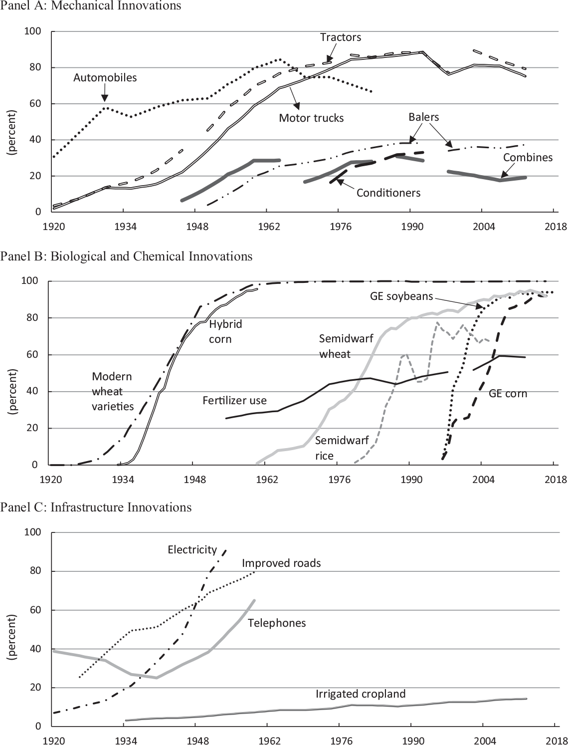
Figure 2 ADOPTION PATHS FOR SELECTED MAJOR U.S. FARMING INNOVATIONS, 1920–2018

Notes: For automobiles, motor trucks, tractors, electricity, and telephone, the data represent the shares of farms using the designated technology. For balers, conditioners, and combines, the data represent the shares of crop farms using the designated technology. For fertilizer, the data represent the share of cropland with fertilizer application. Tractors: From 1920 to 1945, tractors include wheel, crawler, and garden; from 1950 to 1969, tractors include wheel and crawler; from 1978 to 1997, tractors include wheel tractor only; from 2002 to 2012, tractors include wheel and crawler. Automobiles: A drop in the number of automobiles is observed in 1969 and thereafter indicative of a structural change in this measure. See USDA-NASS Census of Agriculture (1969, p. 11) for details. Combines: From 1945 to 1964, combines include pull type and self-propelled; from 1969 to 1982 only self-propelled combines are included; from 1987 to 1992, all types of combine are included; from 1997 onwards, only self-propelled combines are included. Balers: From 1950 to 1992, data refer to pickup balers; from 1997 to 2012, data refer to hay balers. Conditioners: Data refer to mower conditioners. Fertilizer: From 1954 to 1997 fertilizers do not include lime whereas from 2002 to 2012 lime is included. Manure is excluded in all years. From 1978 to 2012, acres on which fertilizers were applied are reported for cropland only, pastureland, and total (i.e., cropland and pastureland). In 1959, 1964, 1969, and 1974, however, data were reported for pastureland and total acres fertilized. Thus, acres of cropland fertilized were estimated for those years by subtracting acres of pastureland fertilized from total acres fertilized. In 1954, only data on total acres fertilized was available. Thus, we estimated the area of cropland fertilized in 1954 by applying the share of cropland fertilized in 1959 to the 1954 cropland area.

Sources: Mechanical and infrastructure innovations data as well as fertilizer data were developed by authors based on estimates from the U.S. Census of Agriculture (Bureau of Census and USDA-NASS, various years). Data for intercensus years were linearly interpolated. Data on hybrid corn are from Alston et al. (Reference Alston, Andersen, James and Pardey2010); GE soybeans and GE corn data are from USDA-NASS “June Agricultural Survey” from 2000 to 2018 and available at www.ers.usda.gov/data-products/adoption-of-genetically-engineered-crops-in-the-us/. Areas of semidwarf wheat and rice, and area of wheat varieties released after 1920 are unpublished data from InSTePP.

Biological innovations, in particular, improved crop varieties (Figure 2, Panel B) that were responsive to chemical fertilizers, took center stage a little later—although they were clearly part of the story all along (Olmstead and Rhode 2008). The archetype example is hybrid corn which transformed agriculture in the American midwest. As a result of focused research over several decades (Alston et al. Reference Alston, Andersen, James and Pardey2010, pp. 264–5) hybrid corn was introduced to farms in Iowa in the early 1930s, although it took until the 1960s for vastly improved hybrids to achieve 100 percent adoption across the United States (Griliches Reference Griliches1957; Dixon Reference Dixon1980; Hallauer and Miranda Filho 1981). These innovations laid the foundation for genetically modified (GM) hybrid corn varieties to be developed and adopted, beginning in 1996 (Fernandez-Cornejo et al. 2014).

Similar, although typically not quite as dramatic, genetic innovations were common to many other agricultural crop and livestock species (especially poultry, see Peterson Reference Peterson1967), and contributed to the rapid rise of yields and aggregate productivity during the second half of the twentieth century (Olmstead and Rhode 2008). Changes in intellectual property rights applied to life forms encouraged private investments that drove much of the downstream genetic gains, especially more recently (Wright and Pardey 2006).

In parallel with these genetic changes was the development of modern agricultural chemicals, including various fertilizers, pesticides, herbicides, antibiotics, and hormones, much of which took shape after WWII (Smith Reference Smith1979; Alston and Pardey 2006). The early twentieth century invention of the Haber-Bosch process for the economical manufacturing of synthetic nitrogen fertilizer, in particular, was profoundly important for enhanced crop yields, especially when combined with complementary genetics and crop management practices. The U.S. on-farm adoption process for these fertilizers and associated varieties was mostly decades later. These were also largely private innovations and interlinked with private and public investment in complementary varietal innovations (e.g., herbicide-tolerant crop varieties) (Pardey and Beddow 2013).

More recently, much agricultural innovation has emphasized information technologies, including various applications of computer technologies, geographic information systems and related precision production systems, satellites, remote- and ground-sensing, and the like. Adoption processes for these digital farming technologies are still in their early and slow stages, apart from relatively simple technologies—that involve neither large investments in specialized equipment or human capital nor major changes in farming systems and practices—such as global positioning system (GPS)-based remote-sensing and guidance systems (e.g., Alston and Pardey 2020).

As well as these on-farm changes, farmers benefited from improved technology for long-distance transportation of farm output, including refrigeration and preservation technologies, coupled with investment in roads, railroads, and other public infrastructure (Fogel Reference Fogel1964; Atack Reference Atack2013). Public infrastructure investments that contributed considerably to agricultural productivity include those related to rural electrification, telephone service, and irrigation projects (e.g., Beall Reference Beall1940; Fischer Reference Fischer1987).Footnote ¹⁹ These infrastructure improvements and other off-farm changes complemented on-farm innovations (e.g., Figure 2, Panel C).

A Mid-Century Surge in Technology Adoption?

Table 3 reports the growth in adoption rates (share of farmers or farm area adopting) for major examples of each of the main categories of innovation. Growth rates are reported for terciles of the century, 1920–2018. If the mid-century surge in productivity growth was associated with a contemporaneous surge in adoption of innovations, we should see a surge in adoption in the middle tercile (1940–1980), compared with the first (1920–1940) and third (1980–2018) terciles. The patterns in Table 3 are consistent with Figure 2. Adoption of several major mechanical innovations and infrastructure improvements (tractors, trucks, electricity, and improved roads) was fastest in the first tercile, but for some complementary innovations (balers, combines, and conditioners) adoption accelerated in the second tercile. Likewise, for some major biological innovations (hybrid corn and use of fertilizer) adoption grew most rapidly in the first tercile. However, for other crop varietal technologies that came later, adoption accelerated in the second tercile (semi-dwarf wheat and rice) or even later (GM corn and soybeans).

Table 3 GROWTH RATES IN ADOPTION OF SELECTED INNOVATIONS BY TERCILE, 1920–2018

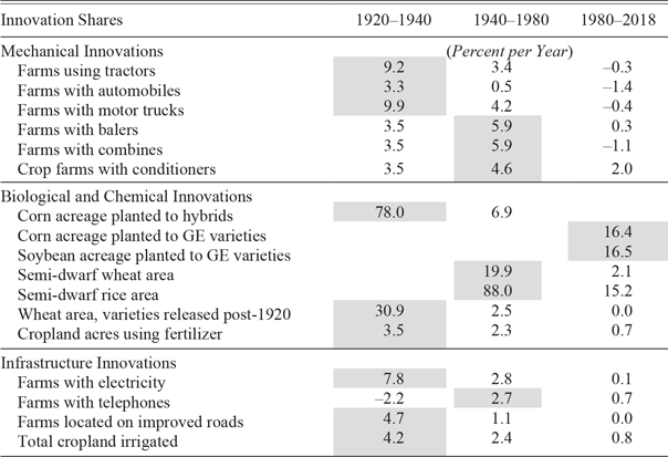
Notes: Shading indicates the tercile with the fastest annual rate of innovation uptake.

For all machinery variables, irrigation and fertilizer, we assumed a share of 0 percent in 1900 and interpolated the data between 1900 and the first year of data available from the Agricultural Census. For GE corn and GE soybeans, we assumed a share of 0 percent in 1980 and interpolated between 1980 and 1996 (first year of data available). For electricity and telephone, we assumed 100 percent of farms had electricity and telephones in 2018 and we interpolated between the last year of data available and 2018. For improved roads, we carried over the 1959 estimate (last year of data available to 2018).

Share of farms using tractors: Last year of data is 2012, so for 1980–2018, growth rates refer to 1980– 2012. Share of farms with automobiles: Last year of data is 1982, so for 1980–2018, growth rates refer to 1980–1982. Share of farms with motor trucks: Last year of data is 2012, so for 1980–2018, growth rates refer to 1980–2012. Share of farms with balers: Last year of data is 2012, so for 1980–2018, growth rates refer to 1980–2012. Share of farms with conditioners: Last year of data is 1992, so for 1980–2018, growth rates refer to 1980–1992. Share of corn planted to hybrids: For the 1920–1940 period, growth rates refer to 1933–1940; for the 1940–1980 period, growth rates refer to 1940–1960. Area share of wheat to semi-dwarf wheat: Last year of data is 2016, so for 1980–2018, growth rates refer to 1980–2016. Area share of rice to semi-dwarf rice: Last year of data is 2005, so for 1980–2018, growth rates refer to 1980–2005. Area share of wheat with varieties released after 1920: Last year of data is 2016, so for 1980–2018, growth rates refer to 1980–2016. Share of cropland using fertilizer: Last year of data is 2012, so for 1980–2018, growth rates refer to 1980–2012. Share of irrigated cropland in total cropland: Last year of data is 2012, so for 1980–2018, growth rates refer to 1980–2012.

Source: See Figure 2.

Taken together, the data in Table 3 and as represented in Figure 2, are consistent with our story about a slowdown in the rate of adoption of innovations contributing to a slowdown in productivity, but they do not clearly concord with a surge in the middle tercile (1940–1980). However, the measured rate of adoption might not accurately reflect the ultimate consequences of these innovations, for three reasons. First, the share of farmers adopting or acres using an innovation might not well match the share of output produced using the technology. Second, economies of size and specialization associated with some of these innovations—especially mechanical innovations—meant that fully realizing the productivity potential required changes in the structure of agriculture and complementary off-farm assets and institutions. Third, it took time to make those structural changes because of the sticky nature of rural resources and the associated costs of change.

The upshot is that the productivity-enhancing consequences of innovation might lag considerably behind the evidence on initial adoption, which itself lags behind research investment. The overall lag between investments in research and its ultimate economic impacts has several elements. First, comes the lag between investing in research and developing technology. Next, comes the lag between the release and initial adoption of technology and its ultimate impact on productivity. This lag is extended when we allow the role of work to adapt technology to better match particular contexts (e.g., as illustrated by the slow spatial diffusion of hybrid corn, particularly as its use extended beyond the corn belt). Last, comes the lag associated with the adjustment process. During this in-between time, in the middle of the twentieth century, while some farmers had adopted innovations and flourished, many others lagged and fell behind. Those who were slow to adjust and exit agriculture contributed to what became known as the farm problem.Footnote ²⁰

STRUCTURAL TRANSFORMATION

The farm problem—excess capacity in agriculture, especially too many farmers—was eventually resolved through consolidation of farms into more economic-sized units, more specialized in particular outputs. This consolidation was enabled and promoted by the adoption of innovative technologies. Especially important were labor-saving machines that enabled considerable economies of size with respect to land and required much less labor to efficiently operate a larger farm area. It took time for the farm sector to absorb these changes and capitalize on the associated efficiencies. Hence, during the decades following the first introduction of those innovations, American agriculture faced a serious adjustment problem—how to move resources out from agriculture, especially labor, that were earning very low returns in farm production where they were stuck.Footnote ²¹ In this section we document the linkage between the structural adjustment process, and the surge and slowdown in farm productivity growth.

Labor-Saving Technologies

Much of the measured productivity gains, especially in the earlier period, can be attributed to mechanization. These were often labor-saving innovations that facilitated the consolidation of farms into many fewer and larger units. Total land in agriculture continued to increase until the early 1950s, but has trended down slowly since then. Meanwhile, average land per farm continued to increase as the number of farms shrank from its peak (6.8 million farms in 1935). In 1910, labor used in agriculture began to decline from its peak plateau (around 10.4 million labor years 1900–1910). The adoption of horses and mules, both to substitute for and complement human labor, transformed agriculture in the second half of the nineteenth century (Olmstead and Rhode 2001). At the turn of the century, the process of replacing animal power with machines had barely begun; in 1910, the United States had a total of 6.4 million farmers, farming 881 million acres using a total of 24 million horses and mules and just 1,000 tractors (Figure 3). Various mechanical innovations had been adopted in the latter nineteenth century and early twentieth century that were powered by horses, but the internal combustion engine really made its presence felt in the decades to come. The tractor, in particular, saved millions of acres of land and the work of many men and women.

Figure 3 U.S. FARM AREA, FARM LABOR, AND FARM NUMBERS, 1850–2018

Note: For number of farms, intercensal values were estimated using a linear interpolation when no value was reported.

Sources: 1850, 1860, 1870, 1880, 1890, and 1900 values for numbers of farms and land in farms are from the U.S. Bureau of the Census (1975, series K-4 and K-5). The 1910 value for land in farms is from series K-5 of the same resource. Number of farms (1910–1999) and land in farms (1911–1999) are from Olmstead and Rhode (2006c, series Da4 and Da5, respectively). For both numbers of farms and land in farms, values for 2000–2018 are from USDA-NASS (2019). Labor data were calculated by the authors using data on persons engaged in production from BEA (2020a), on unpaid family workers from Carter and Sutch (Reference Sutch2006) and Sutch (Reference Sutch2006), and on engaged persons from Kendrick (1961).

As shown in Figure 4 the stock of workhorses and mules on U.S. farms peaked in 1917 at 27 million animals (or 5.5 animals per 100 acres of improved land) dropping steadily to just 3.6 million animals (0.8 per 100 acres of cropland) by 1957, and eventually to a low of 1.4 million in 1974.Footnote ²² Numbers of equines have risen subsequently to more than 4 million, but these are mostly not workhorses and mules; more for recreational use.Footnote ²³ This post-1917 pattern of change in the use of traction animals on farms is the mirror image of tractor use in U.S. agriculture. From just 50,000 tractors in 1917, the total grew to 4.6 million tractors in 1957. After a peak at 4.8 million, beginning some 10 years later the total number of tractors has fluctuated around a slight downward trend. This declining trend reflects several factors, including a decline in the total number of farms, an increase in the average size of farm tractors (thus enabling tractors to work more land per season), and an increase in the provision of third-party contract tractor services.

Figure 4 AMERICAN AGRICULTURAL MECHANIZATION, 1867–2012

Note: See Alston et al. (Reference Alston, Andersen, James and Pardey2010, p. 29) for details on equine stock.

Sources: Equine stock: 1867–2002 from Alston et al. (Reference Alston, Andersen, James and Pardey2010); 2007 and 2012 from USDA-NASS (2019). Other values were linearly interpolated. Tractors: 1910–1990 from Alston et al. (Reference Alston, Andersen, James and Pardey2010); 1991–2007 from FAO (2017); 2012 from USDA-NASS (2014b, table 48); 2008–2011 were linearly interpolated. Combines: 1910–2002 from Alston et al. (Reference Alston, Andersen, James and Pardey2010); 2007 and 2012 from USDA-NASS (2014b, table 48); 2003–2006 were linearly interpolated.

Machines were important in saving land from having to be used to produce feed for horses and mules. Olmstead and Rhode (2001, p. 665) report that “In 1939, 65 million acres of cropland were used to feed horses and mules, with all but 2 million acres devoted to farm stock. By 1960, only 5 million acres were needed.”Footnote ²⁴ However, we suspect a larger driver of farm mechanization over the longer term was its labor-saving implications, motivated by high off-farm labor wage rates driven by innovation in the manufacturing industry and the associated broader economic growth (Kislev and Peterson 1982, 1996; Gardner 2002; Gordon 2016; MacDonald Reference MacDonald2020).Footnote ²⁵ A particular feature of this process was to move people and labor off farms, either entirely or through a substantial increase in part-time farming, and thereby to reduce the relative importance of labor as a farming input—a one-time transformation of agriculture that was largely completed by 1980.

Farm Numbers and Land per Farm

Taking our farm problem perspective, we might expect to see an acceleration of farm productivity growth associated with an acceleration in the rate of farmer exit, enabling the consolidation of farms into larger and more specialized operations (see also MacDonald, Hoppe, and Newton 2018). To check this idea, informally, we estimated cubic logarithmic trend models of the total number of farmers, using data for individual states, USDA regions, and the nation as a whole for the years 1910–2010. These models generally fit well, and they are consistent with an acceleration and slowdown in the rate of decline of farm numbers (i.e., the coefficients on the linear, quadratic, and cubic terms are all highly statistically significant and with the expected signs). Using these results, we solved for the inflection point, as an indication of the year of the peak rate of farm exit, as predicted by the model, and a 95 percent confidence interval around that year.

Table 4 summarizes estimates using state-level data for various spatial aggregates. The disaggregated statistics provide a regionally more nuanced interpretation of the aggregate picture in Figure 3. In each model referring to a particular spatial aggregate, the peak exit year is estimated with high precision (i.e., the 95 percent confidence interval is very narrow, often plus or minus one year) and, across aggregates, the estimates fall within a remarkably narrow range. Pooling the data across all 48 contiguous states, the year of peak exodus was 1959 (between 1958 and 1961 with 95 percent confidence). The spatial pattern is plausible. Across the nine USDA divisions, the year of peak exodus rate ranged from 1956 (New England) to 1964 (West North Central). In every region, the pattern is consistent with a surge in farm exodus in the 1950s and 1960s that conforms with the observed surge in MFP. Average acres per farm peaked a little later because—as shown for the nation as a whole in Figure 4—total land in farms continued to grow for a decade or two after the number of farms had begun to fall.Footnote ²⁶

Table 4 YEARS OF PEAK RATES OF CHANGE IN U.S. FARM NUMBERS AND FARM SIZE, 1910–2012

Sources: Created by the authors based on pooled estimates of cubic trend models using state-level data in logarithms for all of the states within the respective U.S. region. Regions are defined in USDA (2019). Regression results are reported in Online Appendix Table D-5.

Table 5 DISTRIBUTION OF LAND IN FARMS AND NUMBER OF FARMS IN THE UNITED STATES BY AREA PER FARM COHORTS, 1870–2012

Note: Percentages calculated by authors from reported distributions of farm numbers and area.

Source: Authors’ calculations using data from Haines, Fishback, and Rhode (2018).

These national and regional averages and aggregates encompass highly diverse farm sizes and types, both changing over time.Footnote ²⁷ Over time, farms became increasingly specialized in a narrower range of market goods. Many productive activities progressively shifted off farms—to be under-taken by specialized (pre-farm) agribusiness firms that nowadays produce farm machinery, seed, chemicals, energy, and other inputs (including contract services) that were once largely (and in some instances entirely) produced on-farm. Likewise farm households once made many food and fiber products that are now produced entirely off-farm by agribusiness firms in other (post-farm) sectors of the economy. These shifts have implications for where the lines are drawn in distinguishing between farms and other firms and thus between agriculture and the rest of the economy. However, the available data on these shifts are limited, and we work with conventional measures based on statistical definitions of farms.Footnote ²⁸

In 1920, the United States had 735 million acres on 6.4 million farms, at an average of 115.2 acres per farm. Few of those farms had more than 1,000 acres; 58.6 percent had less than 100 acres and used 17.0 percent of the total land in farms, while the other 41.4 percent that had more than 100 acres used 83 percent of the land. By 2012, the total number of farms had fallen by more than two-thirds compared with 1920. Now 8.2 percent of 2.1 million farms had more than 1,000 acres; 54.6 percent had less than 100 acres but these farms used only 4.4 percent of the land, while the other 45.4 percent with more than 100 acres used 95.6 percent of the land. Both tails of the distribution got fatter. Notably, more than 10 percent of today’s farms have less than 10 acres, still, which is surprising given the general push toward larger and more specialized farms. But many of today’s small farms are so-called hobby farms in the urban fringe, and many others at more commercial scale are part-time occupations for people for whom living on a farm is a life-style choice more than a way of making a living.

Because the distribution of land in farms is highly skewed, the simple average may be a misleading indicator of the rate of consolidation of farms. MacDonald (Reference MacDonald2020) demonstrates that the relatively constant number of acres per farm since 1980 reflects increases in both the numbers of very small farms and in the numbers of large farms. He suggests using changes in the midpoint rather than the mean of the distribution of farm size as a more informative indicator of the rate of farm consolidation.Footnote ²⁹ Using this measure, he demonstrates that commodity-specific rates of farm consolidation were generally sustained over the three decades, 1987–2017, and were similar across producers of 55 crops and seven livestock products. While the simple average has barely budged, the midpoint of the distribution of farm size—whether measured in land per farm for cropping farms or numbers of animals for livestock producers—has grown significantly. MacDonald (Reference MacDonald2020) reports annual average growth rates for four commodity classes ranging from 3.01 to 3.59 percent. Thus, while data on the mean might be taken as indicating that the structure of agriculture had stagnated since the 1980s, steady structural change and consolidation has continued, especially among the larger commercial farms that account for the bulk of farm production. This period 1987–2017 is some decades after the maximum rate of farm exit and consolidation revealed by the changes in numbers of farms and land per farm in Table 4.

The Farm Labor Force

Central to these changes in the structure of agriculture have been changes in the structure of the farm labor force, reflecting both labor push and pull phenomena (e.g., Kislev and Peterson 1996; MacDonald Reference MacDonald2020). Growth in the non-farm demand for labor, driving up the opportunity cost of farmers’ time as well as the cost of hired farm labor, pulled people out of farming, while technological changes on farms that permitted more to be produced with much less labor and more land per farm pushed people off the land. Farmers have responded to these incentives and opportunities by consolidating farms and substituting other inputs for labor, in part by developing and adopting labor-saving innovations that favored higher land-labor ratios and larger optimal farm sizes.

Figure 5 captures the main elements of these changes. In Panel A, total labor use in agriculture fell by two-thirds, from 20.5 billion hours in 1949 to 6.3 billion hours in 2007. Within this total, after accounting for the shift to part-time farming, operator labor fell by more than three-quarters, from 13.0 billion hours in 1949 to 3.5 billion hours in 2007, while the hired labor share increased from 19.8 to 31.7 percent. As farmers substituted other inputs—especially material inputs—for more expensive labor, the cost share of labor fell from more than 42 percent in 1949 to less than 30 percent in 2007 (Figure 5, Panel B). Labor still represented a large share of costs, however, since the reduction in labor use only partially offset the cost increases caused by the higher wage rates. One adjustment response of farmers has been to seek off-farm employment for at least one member of the household, which has been facilitated by the growth of the rural non-farm economy. Figure 5, Panel C illustrates. Between 1930 and 2012, the share of full-time farm operators fell from 70 to 40 percent and they increased their average number of days worked off-farm from 86.5 to 144.5.

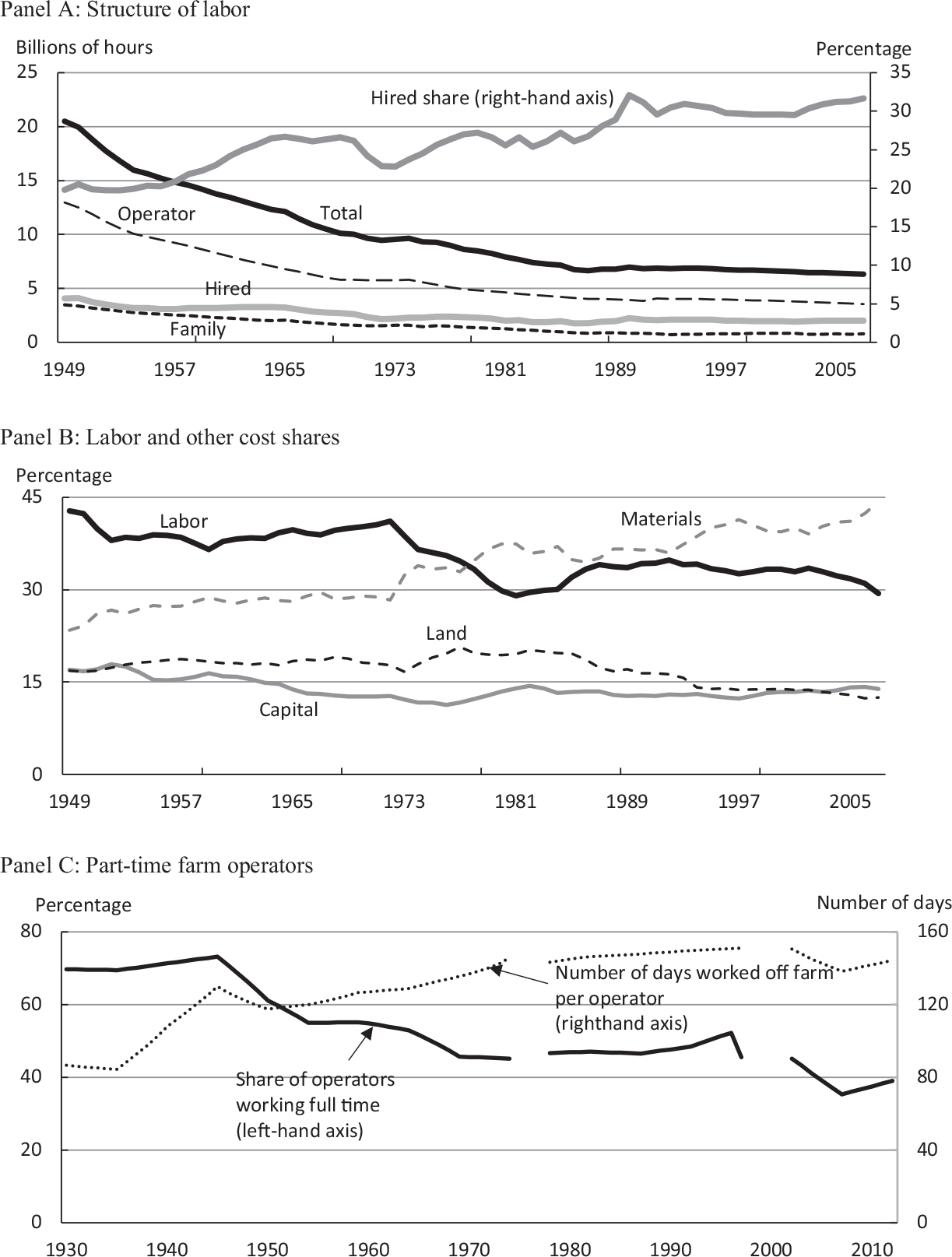
Figure 5 LABOR USE IN U.S. AGRICULTURE, 1949–2012

Notes: In all Census years up to 1997, the reported number of operators was equal to the total number of farms. From 2002 onwards, this is no longer true. The Census collected information on the total number of operators. Therefore, if a farm had more than one operator, it was counted accordingly. In all census years up to 1997, data are reported in terms of operators by days worked off-farm cohorts (e.g., 0 days, 1–49 days, 50–99 days, etc.). For 2002, 2007, and 2012, data are reported in terms of cohorts of days worked off-farm by the principal operator. In 1974, data were collected only for individual or family operations (sole proprietorships) and partnerships. Thus, corporations and other types of organizations (e.g., cooperatives, prison farms, grazing associations, and Indian reservations) were excluded (for more details, see U.S. Bureau of Census 1977, Appendix A, page A4). In all other years, data on days worked off-farm were collected for all types of farms. To calculate the average number of days worked off-farm per operator, we proceeded as follows. First, the total number of days worked off-farm in each cohort was estimated by multiplying the mid-point number of days worked off farm in each cohort (e.g., 25 days for 1–49 days, 75 days for 50–99 days, etc. and 200 days for 200 and more) by the corresponding total number of operators. The total number of days worked off farms was obtained by summing the estimated number of days worked off-farm across cohorts. The number of days worked off-farm per operator is given by the total number of days worked off-farm divided by the total number of operators. Data for intercensal years were estimated by linear interpolation. The total number of operators working full time was estimated by subtracting the number of operators working off-farms from the total number of operators.

Sources: Data for Panels A and B are from the InSTePP Production Accounts, version 5. Data for Panel C were developed by authors based on U.S. Bureau of Census data (various years).

Compared with 1910, commercial farms are now much larger (in 2012, 70 percent of land was on farms exceeding 1,000 acres, up from 23 percent in 1920), and much less labor-intensive. Much of the agricultural transition took place in the middle of the century—between 1930 and 1970; it was associated with an acceleration in farm productivity growth, which has since returned to what seems to be a more normal, long-term rate commensurate with long-term productivity growth in the economy more generally.

PHYSICAL AND REGULATORY ENVIRONMENT

Some other environmental factors might also have contributed to the surge and slowdown of farm productivity growth, reinforcing the consequences of the factors discussed to this point. Specifically, climate change, invasive pests and diseases, evolving pesticide resistance, and declining natural resource stocks could all have contributed to a more challenging physical and economic environment for agricultural production, adding to the demands for maintenance research just to keep yields from falling and costs from rising. Among these possibilities, climate change is an unlikely explanation of the observed productivity patterns prior to 2007 since it has still barely begun to have tangible consequences for agricultural productivity in the United States. But other aspects of the economic environment for producers—including regulations governing production practices on farms—have become more difficult in ways that may help account for the observed phenomenon.

We do not have good data on the size of the associated effects, but the following claims are not controversial: (1) Some of the measured productivity growth reflected unmeasured consumption of stocks of various (often poorly priced) natural resources such that the surge was potentially in part a measurement error. (2) Following the dustbowl, natural resource conservation policies were introduced that internalized some environmental externalities. (3) Over time, environmental policies have been introduced that regulated technologies (especially pesticides and GMOs) and it has become progressively harder to introduce novel technologies that might entail negative externalities (e.g., hazards to human health or the environment). Moreover, state and federal governments are increasingly deregistering individual pesticides and regulating the use of other agricultural chemicals and veterinary medicines. (4) Other technological regulations imposed by government and food chain intermediaries have increasingly restricted production practices related to farm labor, food safety, animal welfare, and the environment (e.g., Saitone, Sexton, and Sumner Reference Saitone, Sexton and Sumner2015). (5) Farmers increasingly have had to pay for varietal technologies they once received for free from public research agencies such that a greater share of the benefits from agricultural R&D are now captured by upstream agribusiness and life sciences firms.

Pesticides illustrate the main ideas here. The surge of farm productivity growth immediately following WWII was associated with a surge in the use of agricultural chemicals, especially synthetic fertilizers and pesticides (Alston and Pardey 2020). Conventional measures of productivity growth do not include adjustments for the negative externalities associated with these agricultural chemicals, and in this sense our measures over-state the true gains in productivity. The publication of Rachel Carson’s Silent Spring in 1962 marks the beginning of the era of public awareness of the environmental consequences of agricultural pesticide use, and environmental regulation of agricultural production. Progressively over the decades since, a great many pesticides have been banned. A direct consequence of these regulations has been to reduce agricultural productivity—both measured and actual. Similar thinking applies to the development of intensive livestock production systems and the progressive, increasingly stringent regulation of the use of antibiotics, hormones, and other veterinary medicines, and regulation of other production practices. These and other regulations seek to protect human health, food safety, animal welfare, endangered species, and other environmental resources; consequences that do not show up in conventional productivity measures.

Together these aspects of the changing natural and regulatory environment confronting farmers might have contributed both to the measured surge (reflecting unmeasured externalities or unmeasured consumption of poorly priced natural resource stocks that contributed to overestimated productivity growth) and to the subsequent slowdown (reflecting the consequences of regulations that internalized some of those costs). It is not easy even to guess at the empirical importance of these aspects, let alone measure them, but they are surely part of the story.