NOMENCLATURE
- 1D
one-dimensional
- ATAG
Air Transport Action group
- BM
bending moment
-
 $$\bar{c}$$
mean aerodynamic chord in m
- CA2LM
Cranfield accelerated aircraft loads model
- CoG
centre of gravity
- DARPA
Defense Advanced Research Project Agency
- DoF
degrees of freedom
- f
intensity distribution function
- F g
flight profile alleviation factor
- FC(s)
flight conditions
- H
gust gradient in m
- HALE
high-altitude long endurance
- HARW
high aspect ratio wing
- IQ(s)
interesting quantities
- LC(s)
loading conditions
- MTOW
maximum take-off weight
- MZFW
maximum zero fuel weight
- n g
vertical load factor in g
- P
structural load of interest
- PSD
power spectral density
-
$$\bar{q}$$
dynamic pressure in Pa
- SF
shear force
- SM
static margin
- TM
torsion moment
- U
velocity
- U ref
reference gust velocity
- UAV
unmanned aerial vehicle
- VFA
very flexible aircraft
- WR
wing root
- x
chordwise/longitudinal co-ordinate
- y
spanwise/lateral co-ordinate


Greek symbol
- α b
fuselage angle-of-attack in °
- θ
aircraft pitch angle in °
1.0 INTRODUCTION
Despite significant investments in the development of more efficient aircraft, overall aerodynamic performance and efficiency have plateaued. However, improvements have been made in engine performances through the use of new technologies. Similarly, on board sub-systems have evolved to provide better performance. Meanwhile, the conventional aircraft layout, i.e. tubular body, swept wings, wing pylon mounted engines, has dominated the aircraft market and design pool, with engineers and researchers continuously improving methods and solutions through many years of experience on similar designs. But major aircraft manufacturers have understood that in order to achieve better performance and reach environmental and efficiency targets( 1 , 2 ), disruptive new concepts must be introduced to supersede the conventional layout.
In fact, the majority of concepts considered for short-term development rely on a coupling between increased wingspan and higher aspect ratio, new propulsion integration methods and some aircraft layout changes. High aspect ratio wings (HARW) are promising because they lead to higher lift to drag ratio compared with conventional wings. The required light weight structures can already be made using a combination of reasonably advanced and mastered manufacturing methods in composite tailoring and alloys. On the other hand, new aeroelastic issues are introduced when compared with wings currently in use. Consequently, flight loads have become an even more critical area of research and extensive use of predictive modelling and simulation is required. For the purpose of gust loads prediction, aircraft concepts are subjected to calculation processes where dedicated gust models derived from atmospheric flight measurements and experimental data are used.
These new aircraft configurations have brought the current gust loads certification processes into question for a number of reasons. The first being that current requirements assume spanwise uniformity of the gust or turbulence. Such simplicity can be explained by an historical analysis of certification model development, originally tailored, in part, to suit low computational power process. Modifications to include non-uniform discrete gust modelling practices seem to have emerged recently for high-altitude long endurance (HALE) unmanned aerial vehicles (UAV) following a number of gust-related structural incidents( Reference Noll, Brown, Perez-Davis, Ishmael, Tiffany and Gaier 3 ). In fact, the impact of the spanwise uniform assumption for both discrete gusts and continuous turbulence was questioned from the start( Reference Houbolt 4 , Reference Hoblit 5 ). But non-uniform models have not yet been introduced in industrial practices and requirements for discrete gust loads of large civil aircraft( 6 , 7 ), despite having equally large wing spans as HALE UAV. Reborn interest in multidimensional derivations from aircraft manufacturers has recently emerged but very little information as to whether it was conclusive for discrete models is available in the literature. Second, gust shapes and intensity were historically derived from vertical accelerations of smaller, more rigid aircraft that exclusively displayed the now conventional layout( Reference Hoblit 5 , Reference Fuller, Richmond, Larkins and Russell 8 ). Consequently, the gust model inherently assumes a similar geometry, despite mass correction factors. Hence, the assumption that the current gust model is applicable to upcoming disruptive concepts, potentially quite different in configuration to reference aircraft( Reference Hoblit, Paul, Shelten and Ashford 9 ) must be revisited and is arguably justifiable by the lack of gust-related incidents. Lastly, higher aspect ratios and wing spans have also pushed the known issue of structural non-linear deflections in large civil aircraft further than ever before. Therefore, innovative load alleviation strategies are investigated using ailerons, spoilers or even morphing wingtips( Reference Guo, De Espinosa de Los Monteros and Liu 10 – Reference Castrichini, Hodigere Siddaramaiah, Calderon, Cooper, Wilson and Lemmens 12 ) for instance. Current spanwise uniform models may not model realistic worst case gust alleviation scenarios, as realistic gust encounters are rarely uniform along the wing. It is also easily conceivable that loads alleviation strategies of highly off-centred devices (outboard ailerons or wingtips) could be improved using non-uniform gust models rather than purely uniform certification models.
This research aims to investigate the effect of using a spanwise non-uniform discrete gust model in the gust loads process of large flexible civil aircraft. This preliminary investigation is based on a conventional layout so as to compare the impact of both uniform (from certification) and non-uniform discrete gust models on loads encountered by an aircraft similar to vehicles currently in operation. It also aims at providing insight into distributed loads alleviation practices when using non-uniform gust models, including a discussion on means and methods to account for spanwise gust non-uniformity.
Within this paper, the authors present a brief overview of the historical development and changes to the discrete gust modelling practices, followed by the introduction of a time-based aeroservoelastic simulation framework used as the main simulation tool. Both the conventional 1-cosine and spanwise non-uniform models are described in detail. Two approaches to gust intensity tuning are introduced. The scope of this paper is limited to a single aircraft configuration used to highlight wing root structural loading, vertical acceleration and pitch changes with gust characteristics during an encounter. Multiple aircraft load cases and flight conditions are used to cover a spectrum of realistic flight conditions. A discussion on the impact of using multidimensional discrete gust models in certification methods, gust loads loop process and load alleviation investigations is presented with the help of time histories and maximum loading of specific quantities using a time domain non-linear simulation framework. Both intensity tuning methods are also compared in terms of resulting loading and relevance to realistic modelling.
2.0 PAST DEVELOPMENTS IN GUST LOADS PREDICTIONS
First mentions of gust loads in aircraft design can be traced back to the 1910s( Reference Wilson 13 , Reference Kussner 14 ). At this very early stage of aviation, gust loads were mainly neglected during aircraft structural design. Only loads due to specific manoeuvres and operational conditions were considered. It was only with the increase in aircraft design speeds and structural weight that gust loads prediction became a crucial part of the design process. A very crude model for gust loads prediction was derived and presented in the 1934 Airworthiness Requirement of Aircraft document( Reference Hoblit 5 , Reference Jones and Connoly 15 ). From that point on, engineers were encouraged to use a sharp edge gust with simple velocity requirements for loads predictions which neglected aircraft motion. It quickly became apparent from experimental findings that gust shape, aircraft motion and general configuration had a great impact on the validity of the loads predictions. Therefore, a new gust model was derived and adopted in 1941 in the main certification process: the linear ramp model. It relied on a gust alleviation factor as a function of wing loading to accommodate for the gust induced motion differences between aircraft. Limitations and differences with realistic gust profiles from flight testing led to yet another new model in 1953: the 1-cosine model, also called the Pratt profile( Reference Pratt 16 ) or isolated discrete gust (IDG)( Reference Jones 17 ). The 1-cosine model replaced the linear ramp as a requirement in 1956( Reference Pratt 16 , Reference Pratt and Walker 18 ). Based on a simple cosine gust shape with intensity tuning specifications, the model relies on atmospheric flight measurements, operational weights and flight conditions at which the aircraft is flown to generate a realistic gust intensity at a given gust gradient. As most civil aircraft had similar characteristics at the time, no need for configuration-type corrections were identified and only aircraft operational mass and dimension are taken into account. A spanwise uniform gust is derived to match realistic worst case scenarios at a given altitude. Measurements to derive the model relied mainly on vertical acceleration and angle-of-attack during the gust encounter. This approach to discrete gust modelling is still used in industry today, with a number of modifications made to the original requirements, and is described CS-25.341(a)( 6 ) (or CFR-25.341(a)( 7 )). No specifications are given to account for disruptive aircraft designs and is inherently limited to a cosine shape. Nevertheless, together with safety factors, the 1-cosine model is accepted as suitable for large localised gust loads prediction and is still used as a design tool today.
Also in the early 1950s, a continuous modelling approach for gusts and turbulence was derived in order to address the problem of modelling realistic turbulence. A power-spectral-density (PSD) formulation was used to represent random turbulence fluctuations using a spectrum of frequencies. To do so, a Gaussian-based intensity distribution around the mean turbulent velocity was used.
Extensive work was carried out in the following decades to develop and lay down the foundations of gust and turbulence loads simulation processes( Reference Houbolt 4 , Reference Hoblit 5 , Reference Press, Medows and Hadlock 19 ). These have led to methods now gathered in the certification requirements and presented in CS-25.341(b)( 6 ) (or CFR-25.341(b)( 7 )). Unlike the 1-cosine model, this approach is not suitable for severe or localised gust cases which can arguably be qualified as more relevant to critical structural design. As a frequency-based method, it is much more relevant for stress and life-cycle studies. Nevertheless, both methods are complementary and must be used for aircraft certification purposes.
In parallel, numerous studies focusing on means to upgrade the spanwise uniform continuous turbulence model have been undertaken. In fact, the spanwise uniform assumption of turbulence has been challenged repeatedly. Diederich( Reference Diederich and Drischler 20 ) focused on the effect of spanwise variation of gust intensity on lift acting on the aircraft. The addition of the multidimensional parameters to define turbulence intensity and direction is justified by the concept of turbulence isotropy. Turbulence intensity and direction were given a random distribution in all axis( Reference Eichenbaum 21 – Reference Pratt 23 ) which led to a variation in predicted gust loads. Simulations applied to Concorde( Reference Coupry 24 ) displayed significant load reduction and aircraft life management implications. It should be noted that Coupry chose to investigate the Concorde, which can only be qualified as an unconventional civil aircraft: quite different in shape, technology, aerodynamics and operational conditions from contemporary models, it was an ideal candidate for his investigations on gust modelling certification applicability. L1011 results( Reference Hoblit 5 ) indicated increased wing torsion inboard of the engines in the worst case scenarios. Focusing only on turbulence or continuous loads, these studies were found to be computationally expensive at the time of their publication, a conclusion that can now be challenged. More recently, a multi-dimensional gust analysis of a large flexible aircraft( Reference Teufel, Hanel and Well 25 ) investigated the impact of the additional spanwise variation both in open-loop and closed loop simulations in the frequency domain, or continuous gusts. The authors did not outline extensive computational requirement increase of the method, and underlined the modified response of the wing when compared to the spanwise uniform continuous turbulence. Specific spanwise velocity distributions also led to the greater excitation of different modes compared to the uniform model.
In comparison, it appears that little interest was shown to improve the uniform discrete gust loads models. Notable attempts can be found in the form of the statistical discrete gust (SDG) model( Reference Jones 17 , Reference Jones 26 ). This multi-axis extension of the 1-cosine combines both lateral and vertical velocity components and was intended to compete with discrete round-the-clock methods already accepted for certification purposes and multi-axis PSD methods. It aimed at predicting the most severe gust and turbulence loads( Reference Jones 27 ) more efficiently by reducing the number of gust criteria for certification and by introducing a design method able to handle load alleviation and active controls. This meant a re-evaluation of the current certification methods and applications for future commercial aircraft: a long and tedious process. Advisory recommendations to push predictions further can be found( 28 ) but have not been fully adopted and do not constitute or authorise any changes to regulations.
Hence, although great improvements in computational capabilities were made in both hardware and mathematical models, the complexity of the certification 1-cos discrete gust model remained almost identical over the 70 years of existence of the method. Specifications to make the simple symmetrical spanwise uniform sinusoidal gust shape more complex by combining gust directions in round-the-clock methods can now be found, but the intensity tuning method and overall gust shape limit the model complexity. Note that whilst the certification documents specify that symmetric gusts must be used in the case of gust loads simulation, the limitation to spanwise uniform loading is never specified as such. Nevertheless, no indication or method to model a spanwise non-uniform gust is given, which arguably constitutes a shortfall of the method when designing flexible structures. After all, these requirements were designed to reproduce realistic yet simplified worst case scenarios from historical flight data obtained on conventional configurations.
Engineers have put together a number of different aircraft concepts over the years, with some more disruptive in layout and technology than others. Compared to Prandtl boxed wings (PBW), blended wings (BW) or forward swept wings (FSW)( Reference Seitz, Kruse, Wunderlich, Bold and Heinrich 29 , Reference Krüger, Klimmek, Liepelt, Schmidt, Wait and Cumnuantip 30 ), some HARW concepts such as NASA SUGAR( Reference Bradley and Droney 31 ) can actually be considered as very similar to currently flown aircraft. But in reality, the aeroelastic response of the flexible structure and increased aspect ratio of the wings leads to reasonable doubts on whether the historical discrete gust model is suitable for configurations that can exhibit non-linear aeroelastic phenomenon. In fact, incidents linked to turbulence induced aeroelastic phenomena have already been encountered on HALE UAV: the Helios aircraft which suffered a critical structural failure over Hawaii during a flight test( Reference Noll, Brown, Perez-Davis, Ishmael, Tiffany and Gaier 3 ). Post-incident investigations, flight reconstruction and weather models( Reference Porter, Stevens, Roe, Kono, Kress and Lau 32 , Reference Roe, Stevens and Porter 33 ) highlighted an aeroelastic phenomena as the main driver of the incident which occurred when the prototype encountered turbulent conditions during climb behind the landscape wake. Recommendations to modify time-based multidisciplinary aeroelastic modelling techniques were given which led to the Defence Advanced Research Project Agency (DARPA) recommendations on gust models for HALE and flexible aircraft( 34 ). In this document, and as an output of the Vulture II program, DARPA introduced a multidimensional discrete gust model with recommendations for HALE UAV and flexible aerostructures. In parallel, an evaluation of the discrete gust loads certification methods applied to HALE aircraft also led to the identification of modelling errors and invalid assumptions( Reference Ricciardi, Patil, Canfield and Lindsley 35 ) for flexible vehicles. In the latter, the conventional discrete gust model was found unsuitable by the authors for flying wing and recommendations were made for unconventional configurations. Such findings seriously raise the question as to whether the current certification models are applicable to the disruptive concepts mentioned above.
The fact that investigations regarding the convergence of various gust modelling methodologies in higher aerodynamic fidelity simulations( Reference Heinrich and Reimer 36 , Reference Kaiser, Thormann, Dimitrov, D. and Nitzsche, J. 37 ), comparisons to lower fidelity approaches( Reference Reimer, Ritter, Heinrich and Krüger 38 ) or even development of unified manoeuvre and gust loads for flight dynamics analysis( Reference Kier and Looye 39 ) are still very much on-going is a tribute to the importance of gust loads analysis in aircraft design. But in these investigations, and the overall trend in current industrial and academic practices, gust loads model almost exclusively rely on conventional discrete uniform models when looking at large civil aircraft. For instance, work led by DLR on an Airbus XRF-1 experimental development aircraft model( Reference Krüger and Klimmek 40 ) included a spanwise uniform model. This is true even in innovative research projects: it was applied on a large transport FSW concept( Reference Krüger, Klimmek, Liepelt, Schmidt, Wait and Cumnuantip 30 ), effectively making the assumption that the worst case discrete gust was also spanwise uniform in this unconventional configuration. Investigations regarding innovative gust loads control( Reference Guo, De Espinosa de Los Monteros and Liu 10 ) or the use of multi-surface control strategies( Reference Ricci and Scotti 41 ) also used spanwise uniform assumptions.
Only investigations on HALE concepts have published results involving multidimensional discrete gust models as described by DARPA. The effect of structural stiffness variation on a very flexible aircraft (VFA) longitudinal flight dynamics and structural loading interest quantities (IQs) were investigated using a multidimensional discrete vertical gust definition( Reference Dillsaver, Cesnik and Kolmanovsky 42 ). Another study of a VFA focused on the reduced order modelling of the vehicle in both spanwise uniform and non-uniform gust (in an asymmetric configuration)( Reference Hesse and Palacios 43 ). These studies mainly focused on the aeroelastic effects of using a spanwise non-uniform model on a VFA, not on the derivation or consequences of using such approaches to conventional gust loads processes. In fact, both focused on time domain simulations of a single spanwise intensity definition, designed to apply the critical wing root bending moment. Both also used the single amplitude correction derived by DARPA for VFA concepts which accounts for the spanwise variation effects( 34 , Reference Dillsaver, Cesnik and Kolmanovsky 42 , Reference Hesse and Palacios 43 ).
All in all, multidimensional discrete gust models for large civil aircraft have not been widely investigated or published, despite recent developments made for HALE UAV( 34 ) and recommendations for caution in non-conventional configurations.
3.0 FRAMEWORK AND GUST MODEL SET-UP
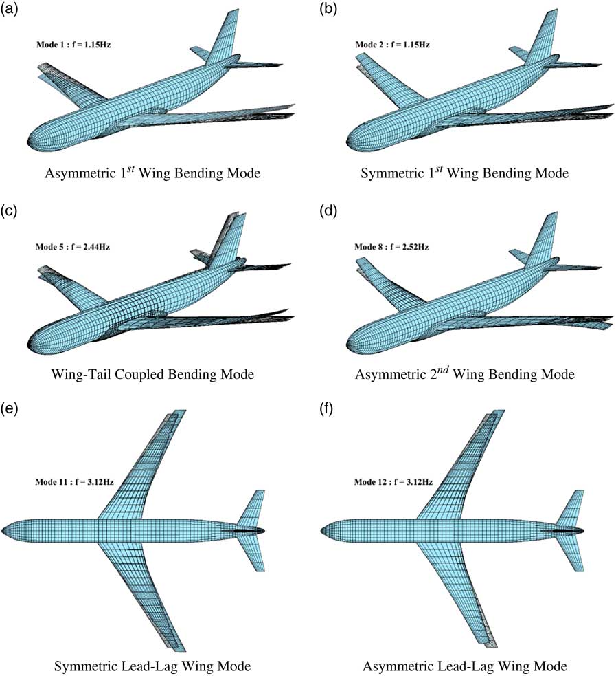
The Cranfield Accelerated Aircraft Loads Model (CA2LM)( Reference Andrews 44 ) framework can be used to investigate discrete gust loads analysis of large flexible aircraft. This time-based aeroservoelastic simulation framework couples both linear structural flexibility and unsteady aerodynamics in near real-time simulations to capture aircraft flight dynamics and other structural loading IQs. The Matlab/Simulink-based tool can also be used for handling quality investigations and was previously used to study realistic pilot models, the effect of manual controls on flexible structures( Reference Lone and Cooke 45 ) and flight loads( Reference Lone, Lai, Cooke and Whidborne 46 ). The general architecture of the framework is given in Fig. 1. For the aerodynamic model, the unsteady aerodynamics are based on a modified strip theory, corrected for non-infinite span conditions( Reference Andrews 44 ). Unsteady terms are introduced using a Leishman–Beddoes formulation, effectively introducing a time lag and flow build up effects on angle-of-attack( Reference Andrews 44 , Reference Dussart, Portapas, Pontillo and Lone 47 ). Additionally, tail downwash is included along with empirical fuselage, engine/nacelle and wing-body aerodynamic interaction models from empirical scientific data units. Note that the aerodynamic model, therefore, assumes that no shock occurs at any of the lifting surfaces aerodynamic sections. A simple Prandlt–Glauert compressibility correction is applied, effectively limiting the model to Mach numbers of 0.7. The steady aerodynamic results of the modified strip theory were validated against a full 3D CFD analysis( Reference Carrizalez, Dussart, Portapas, Pontillo and Lone 48 ) of the aircraft. For the structural model, a linear modal approach is used to deform the complete vehicle. The latter is idealised as a beam structure with distributed mass and stiffness properties and includes both elastic and inertial couplings. Both aerodynamic and structural models are coupled using an iterative process and a mean-axes system to decouple rigid-aircraft motion and structural flexibility when solving the equations of motion of the aircraft. Illustrative examples of mode shapes and frequencies of the simplified aircraft structure, precomputed prior to any flight simulation using an in-house linear Euler Bernoulli solver, are shown in Fig. A1. Updated centre of gravity (CoG) positions with structural flexibility and forces and moments acting on the airframe are used to compute aircraft positions, velocities and accelerations in all six degrees of freedom (DoF). Aircraft position is used in both gravity and atmospheric condition models to complete the simulation environment. For a more detailed description of the framework, the reader is referred to the dedicated literature( Reference Andrews 44 , Reference Dussart, Portapas, Pontillo and Lone 47 , Reference Andrews and Cooke 49 – Reference Portapas, Cooke and Lone 51 ) which covers the modelling assumptions in greater details.
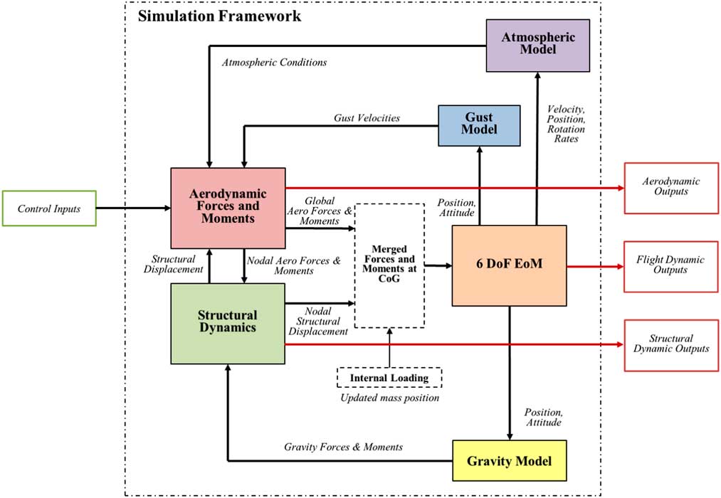
Figure 1 General architectural diagram of the CA2LM framework.
Additionally, a continuous turbulence and discrete gust model can be used for gust load predictions. In this model, velocity disturbances are applied to the entire set of distributed aerodynamic stations used for the aerodynamic loading calculations. The individual position and velocity of each station relative to the aircraft reference frame and aircraft CoG position, and aircraft velocity relative to the Earth reference frame are used to determine the resulting distributed disturbance velocities at each time step. Figure 2 illustrates a beam structural model of the aircraft before penetration of a spanwise uniform vertical gust velocity field represented by a continuous surface. The model allows for purely vertical, longitudinal or lateral gust directions, or a combination of both lateral and vertical vectors for round-the-clock simulations. All 6 DoF are given to the aircraft whilst penetration effects are inherently modelled with spatial and temporal distributed loading. The local disturbance velocity is converted to a local angle-of-attack and effective flow speed modification for each station which will lead to a change in the station aerodynamic loading.
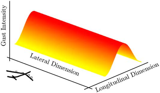
Figure 2 Illustration of a conventional spanwise uniform gust.
3.1 Conventional uniform Pratt model
In order to generate the distributed velocity field, a single time invariant signal is generated based on regulation specifications( 6 , 7 ). The discrete gust is derived using
 $$U_{{{\rm dg}}} (x_{d} ){\equals}U_{{{\rm do}}} {\times}f_{x} (x_{d} ,H_{x} ){\equals}U_{{{\rm do}}} {\times}{1 \over 2}\left( {1{\minus}\cos {{\pi x_{d} } \over {H_{x} }}} \right)$$
where U dg(xd) is the resulting disturbance velocity, U do is the discrete gust reference or design velocity obtained using
 $$U_{{{\rm do}}} {\equals}U_{{{\rm ref}}} .F_{g} .\left( {{{H_{x} } \over {107}}} \right)^{{1/6}} $$
where U do is the design gust velocity, U ref is the reference gust velocity, specified as a function of altitude. F g is the flight profile alleviation factor which serves as a correction to U ref as a function of altitude. The expression for F g is given in CS-25.341(a)(6)( 6 ). H x is the gust gradient, or half gust length, and x d is the node position along the Earth longitudinal axis. A sufficient number of gust gradients ranging from 9 m to 107 m (30–350 ft)( 6 ) must be used. In the case of high mean geometric chord, specifications recommend to push the maximum gust gradient to an empirical 12.5 times the mean aerodynamic chord in order to capture the complete loads envelope. It is also recommended to push the range of gust gradients until maximum IQ values are reached and assess if these can be found within reasonable margins of the certification limiting gust lengths.
3.2 Multidimensional non-uniform model
In order to model a spanwise non-uniform loading, Eq. (1) was modified based on the principle of atmospheric isotropy( Reference Houbolt 4 , Reference Hoblit 5 ), which states that any assumptions made on gust chordwise definition are applicable to all spatial directions and independent of aircraft heading. This can be argued on larger scales, especially in the vertical direction as altitude plays a greater role in atmospheric property changes as latitude and longitude. Nonetheless, the lateral (spanwise) and longitudinal (chordwise) parameters are therefore treated equally. Therefore, a spanwise distribution function f y mimicking f x is coupled into the model such that Eq. (1) becomes
 $$U_{{{\rm dg}}} (x_{d} ,y_{d} ){\equals}U_{{{\rm do}}} .f_{x} (x_{d} ,H_{x} ).f_{y} (y_{d} ,H_{y} )$$
where x d and y d are now, respectively, the longitudinal and lateral co-ordinates of the aircraft in the earth reference frame, H x and H y are the gust gradient in both directions, assumed independent from one another and to follow the certification gust length recommendations ranging from 9 m to 107 m or 12.5 times the mean aerodynamic chord. Note that, like f x , f y is not a time dependant function: time dependency is introduced by the motion of the aircraft through the gust. Two different spanwise distribution functions f y are illustrated in Fig. 3(a) and (b).
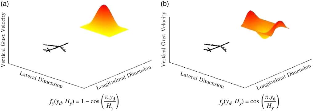
Figure 3 Illustrative f y function examples of spanwise non-uniform gusts.
Different options can be used to scale the maximum gust intensity U do: the conventional or single-gradient method, based only on the chordwise gust gradient H x as given in Eq. (2), and an isotropic or multi-gradient method using the largest of H x and H y gradients, formulated in Eq. (4). Both will be investigated and compared in respective results section:
 $$U_{{{\rm do}}} {\equals}\left \{ {\matrix{ {\;\;U_{{{\rm ref}}} .F_{g} .\left( {{{H_{x} } \over {107}}} \right)^{{1\,/\,6}} } & {{\rm if}\;\;\;H_{x} \geq H_{y} } \hfill \cr {\;\;U_{{{\rm ref}}} .F_{g} .\left( {{{H_{y} } \over {107}}} \right)^{{1\,/\,6}} } & {{\rm if}\;\;\;107\geq H_{y} \geq H_{x} } \hfill \cr {\;\;U_{{{\rm ref}}} .F_{g} .\left( {{{107} \over {107}}} \right)^{{1\,/\,6}} } & {{\rm if}\;\;\;H_{y} \geq 107} \hfill \cr } } \right.$$
Additionally, it is possible to rotate the gust lateral and longitudinal axes around the vertical axes if an asymmetric penetration is desired. Independent offsets in both directions are also possible for gust placement relative to the aircraft by simply adding an additional phase term. Gust direction can be set to either vertical, lateral, longitudinal, a combination of any and normalised round-the-clock combinations. By selecting carefully the distribution functions f x and f y , total velocity direction can be set to vary locally if desired. In this study, only a head on vertical gust is investigated.
4.0 SIMULATION PARAMETERS AND TEST CASES
4.1 Aircraft model details
The aircraft that was selected for this specific study is the Cranfield University AX-1, which is effectively a close derivative from the Airbus eXperimental Research Forum model XRF-1 also found in other literature pieces( Reference Timme, Badcock and Da Ronch 52 , Reference Kroll, Abu-Zurayk, Dimitrov, Franz, Führer, Gerhold, Görtz, Heinrich, Ilic, Jepsen, Jägersküpper, Kruse, Krumbein, Langer, Liu, Liepelt, Reimer, Ritter, Schwöppe, Scherer, Spiering, Thormann, Togiti, Vollmer and Wendisch 53 ). Generic details of the aircraft geometry can be found in Fig. 4. Additionally, Fig. 5 illustrates the aircraft’s beam model, with specific mass, structural node and aerodynamic station distribution. Stiffness parameters of the wing structure are also slightly different so as to emphasise the aeroservoelastic effects within the framework. With a wingspan of 29 m, the aircraft wingtip elastic deformation in cruise flight and gust encounter are approximately 2.4 m and 3.1 m above the aircraft jig shape. This effectively keeps deflection below the 10% of wingspan mark in cruise and slightly over during gust events, which is generally accepted as the limit of linear structural behaviour.
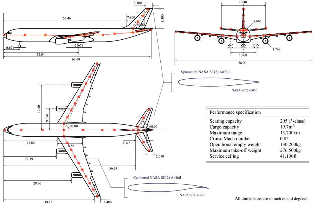
Figure 4 Cranfield University AX-1 large long range aircraft.
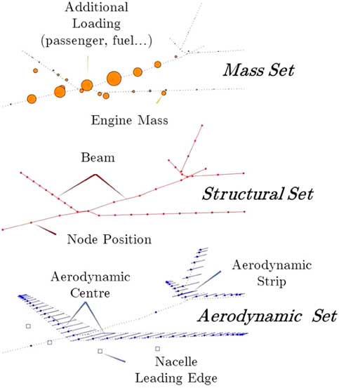
Figure 5 Discretised model.
4.2 Test conditions
Open-loop simulations, as prescribed by certification requirements, will be presented here for a single aircraft configuration at two specific mass cases given in Table 1. In the first case, the aircraft is loaded to near maximum take-off weight (MTOW) in a heavy take off configuration where the CoG position lies within the static margin (SM) of the aircraft at 22% of the mean aerodynamic chord. The second case considers the aircraft loaded near the maximum zero fuel weight (MZFW) with a similar static margin (19%) so as to model a heavily loaded landing scenario. This ensures that both scenarios are realistic and that the aircraft naturally converges back to a stable state after the gust encounter in the open loop simulations. In other words, the pilot or flight control system is assumed not to compensate for any attitude or motion changes, which could lead to drastically different results in structural loading. Multiple flight conditions (FCs) were selected. Details are given in Fig. 6 and Table 2. Flight points are all located along the design cruise speed envelope for the lower altitude spectrum where dynamic pressures are higher. It also suits the aerodynamic limitations of the framework linked to the modified strip theory and the lack of transonic aerodynamic modelling( Reference Andrews 44 , Reference Lone 50 ). Selected FCs and aircraft loading are also aimed at reproducing isolated worst case gust encounters at normal operating conditions during the ascent and descent phases.
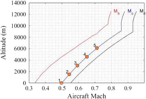
Figure 6 AX-1 Operating flight envelope and selected flight conditions.
Table 1 Aircraft loading details

Table 2 Flight conditions details for the selected conditions

Lastly, the spanwise distribution function selected for this study follows Eq. (5). Gust total velocity is given by Eq. (6) as a function of both lateral and longitudinal co-ordinates of the interest point. This specific distribution allows for a symmetric loading regardless of the gust gradient. Furthermore, it leads to opposite velocity directions between wingtip and root (see Fig. 7(b)) for the lower end of the H y spectrum. The higher end of the H y spectrum converges to a shape similar to that of the uniform 1-cos conventional model (Fig. 7(a)–(d)), justifying a comparison between the two models. Furthermore, the angle-of-attack due to the gust at the fuselage is kept similar regardless of the spanwise gust gradient. On the other hand, changes in gust distribution and subsequent aircraft responses lead to differences in vertical acceleration, pitch and plunging motions during and after the encounter
 $$f_{y} (y_{d} ,H_{y} ){\equals}\cos \left( {{{\pi .y_{d} } \over {H_{y} }}} \right)$$
 $$U_{{{\rm dg}}} (x_{d} ,y_{d} ){\equals}U_{{{\rm do}}} .f_{x} (x_{d} ,H_{x} ).f_{y} (y_{d} ,H_{y} )$$
 $${\equals}U_{{{\rm do}}} .{1 \over 2}.\left( {1{\minus}\cos {{\pi .x_{d} } \over {H_{x} }}} \right).\cos \left( {{{\pi .y_{d} } \over {H_{y} }}} \right)$$
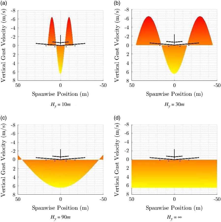
Figure 7 Effect of H y on the discrete gust shape for a given f y distribution.
Only vertical velocity gust encounters are discussed in this paper. Both longitudinal (chordwise) and lateral (spanwise) vertical gust gradients, H x and H y respectively, are varied between identical limits ranging from 9 m to 180 m. The range of gust gradients was increased from 107 m in an attempt to reach an eventual IQ maxima with gust gradient. In the case of the uniform model, the model neglects the H y value and applies a spanwise uniform loading. Both upward and downward gust cases are compared so as to capture the vertical worst case scenario. In order to capture spanwise variation effects whist keeping a relatively low number of simulations, a non-linear distribution of 16 H y values was selected. Smaller intervals at the lower end of the H y gust gradients were used so as to capture the effect of local vertical velocity direction changes. A linear distribution of 15 H x values is used, similar to conventional recommendations.
4.3 Loads simulation process
A loads loop process was set-up following the logical diagram given in Fig. 8. The use of a spanwise distribution with different gust gradients adds an extra loop to the process, increasing the required amount of simulations proportionally to the number of gust gradients H y , spanwise distribution function and possible local gust direction combinations. With a set of 16 H y gradients (as shown in Fig. 8), process computational time rises by an order of magnitude, regardless of eventual simulation parallelisation when compared with the conventional uniform approach.
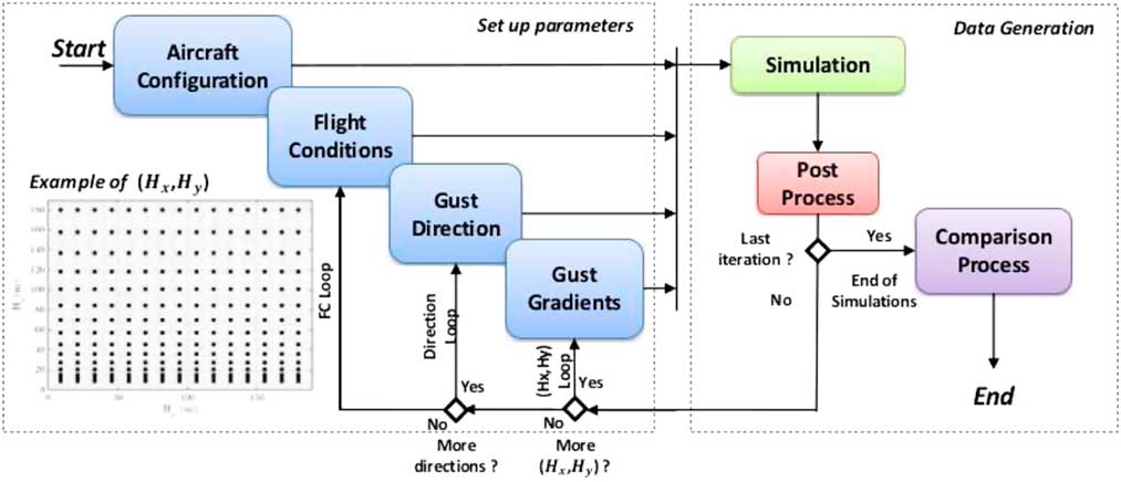
Figure 8 Gust loads loop process diagram.
At the end of each simulation, IQ data are saved. The worst case maximum and minimum loading of specific IQs of each simulation is identified and stored for a batch comparison of results.
5.0 NON-UNIFORM GUST LOADS ANALYSIS
The objective of this paper is to perform a preliminary investigation on the impact of spanwise non-uniform discrete gust model on a large conventional civil aircraft and assess if new worst case scenarios are introduced. Therefore, a comparison between the uniform and the non-uniform model is made and presented in this section. All results discussed were obtained using the conventional intensity tuning method (Eq. (2)) unless stated otherwise in Section 5.4. Primary focus lies on wing root IQs such as bending moment (BM), torsion (TM) and shear force (SF) as well as the aircraft pitch θ and vertical load factor n g which are directly linked to the aircraft response to various gust characteristics.
5.1 Impact of H y on aircraft maximum loading
Ultimately, the metrics used to size the structural limits of the aircraft are the maximum loading quantities encountered during the various gust cases throughout the flight envelope. To efficiently compare the entire simulation batch (which usually involves millions of test cases in industry), the maximum or minimum wing root (WR) load P WR is identified in each of the open loop simulation case, regardless of the time at which it occurs. Additionally, the following normalisation metric is defined:
 $$\Delta P^{{{\rm WR}}} (H_{x} ,H_{y} ){\equals}{{\left( {P_{{{\rm ori}}}^{{{\rm WR}}} (H_{x} ){\minus}P_{{{\rm nu}}}^{{{\rm WR}}} (H_{x} ,H_{y} )} \right)} \over {P_{{{\rm ori}}}^{{{\rm WR}}} (H_{x} )}}$$
where
 $$P^{{{\rm WR}}} (H_{x} ,H_{y} )$$
is the maximum wing root IQ obtained at gust gradients H
x
and H
y
.
$$P^{{{\rm WR}}} (H_{x} ,H_{y} )$$
is the maximum wing root IQ obtained at gust gradients H
x
and H
y
.
 $$P_{{{\rm ori}}}^{{{\rm WR}}} $$
refers to results obtained using the conventional model, whereas
$$P_{{{\rm ori}}}^{{{\rm WR}}} $$
refers to results obtained using the conventional model, whereas
 $$P_{{{\rm nu}}}^{{{\rm WR}}} $$
refers to results obtained with the non-uniform model.
$$P_{{{\rm nu}}}^{{{\rm WR}}} $$
refers to results obtained with the non-uniform model.
 $$\Delta P^{{{\rm WR}}} (H_{x} ,H_{y} )$$
is, therefore, the normalised difference between both methods against the original local maximal load value
$$\Delta P^{{{\rm WR}}} (H_{x} ,H_{y} )$$
is, therefore, the normalised difference between both methods against the original local maximal load value
 $$P_{{{\rm ori}}}^{{{\rm WR}}} $$
. Values should, therefore, range between 1 at maximum difference and 0 when both models are equivalent. The value falls below 0 when the non-uniform model leads to a more extreme local loading. Similarly, the normalised difference against the global maximal load value can be defined as
$$P_{{{\rm ori}}}^{{{\rm WR}}} $$
. Values should, therefore, range between 1 at maximum difference and 0 when both models are equivalent. The value falls below 0 when the non-uniform model leads to a more extreme local loading. Similarly, the normalised difference against the global maximal load value can be defined as
 $$\Delta \tilde{P}^{{{\rm WR}}} (H_{x} ,H_{y} ){\equals}{{\left( {P_{{{\rm ori}}}^{{{\rm WR}}} (H_{x} ){\minus}P_{{{\rm nu}}}^{{{\rm WR}}} (H_{x} ,H_{y} )} \right)} \over {{\rm max}(P_{{{\rm ori}}}^{{{\rm WR}}} (H_{x} ))}}$$
where
 $${\rm max}(P_{{{\rm ori}}}^{{{\rm WR}}} (H_{x} ))$$
is the overall maximum load obtained from the original model for the entire spectrum of chordwise gradients. Therefore,
$${\rm max}(P_{{{\rm ori}}}^{{{\rm WR}}} (H_{x} ))$$
is the overall maximum load obtained from the original model for the entire spectrum of chordwise gradients. Therefore,
 $$\Delta \tilde{P}^{{{\rm WR}}} (H_{x} ,H_{y} )$$
is the normalised difference between any data point of the non-uniform model and the overall maximum loading obtained with the conventional model. Both of the above metrics can be used for different objectives: the first indicates which model leads to higher loads for a given set of gradients whilst the latter compares against the global maximum for the entire set of gradients used in the process. Hence,
$$\Delta \tilde{P}^{{{\rm WR}}} (H_{x} ,H_{y} )$$
is the normalised difference between any data point of the non-uniform model and the overall maximum loading obtained with the conventional model. Both of the above metrics can be used for different objectives: the first indicates which model leads to higher loads for a given set of gradients whilst the latter compares against the global maximum for the entire set of gradients used in the process. Hence,
 $$\Delta \tilde{P}^{{{\rm WR}}} (H_{x} ,H_{y} )$$
can be used for the critical gust load case identification and comparison whilst
$$\Delta \tilde{P}^{{{\rm WR}}} (H_{x} ,H_{y} )$$
can be used for the critical gust load case identification and comparison whilst
 $$\Delta P^{{{\rm WR}}} (H_{x} ,H_{y} )$$
will be used in the direct comparison of models, fatigue and life cycle analysis.
$$\Delta P^{{{\rm WR}}} (H_{x} ,H_{y} )$$
will be used in the direct comparison of models, fatigue and life cycle analysis.
Wing root loading IQ and normalised differences can be presented in the form of surface plots, as illustrated in Fig. 9(a) and (b). Minimum and maximum wing root bending moment are displayed for both models as a function of both gust gradients in Fig. 9(a). Structural loads are given in offset percentage relative to trim values. Results are given for the bidirectional gust loads batch for a given flight condition and loading. The non-uniform model leads to lower wing root bending moment and, therefore, lies below the boundaries defined by the conventional model (transparent grid).
 $$1{\minus}\Delta P_{{{\rm local}}}^{{{\rm WR}}} $$
quantities are given in Fig. 9(b). Both the normalised difference and wing root bending map clearly show that the non-uniform model leads to lower loads prediction. This is true for all aircraft loading and flight conditions included in this study. With increasing H
y
gradients, the non-uniform model converges to the conventional uniform model, as expected from gust velocity trends with gradients presented in Section 3. Furthermore, as H
x
increases, maximum or minimum loading shifts to the aircraft recovery phase (pitch and heave motion), and no longer takes place during the gust encounter. Despite increasing H
x
past the recommended 107 m limit, no maximum loading peak with H
x
was found. Higher loading was achieved during low-altitude gust encounters. Overall, the critical scenario was identified at the sea-level flight with the less fuel, the remaining of which being stored in the fuselage (FC 1 LC 2 set-up).
$$1{\minus}\Delta P_{{{\rm local}}}^{{{\rm WR}}} $$
quantities are given in Fig. 9(b). Both the normalised difference and wing root bending map clearly show that the non-uniform model leads to lower loads prediction. This is true for all aircraft loading and flight conditions included in this study. With increasing H
y
gradients, the non-uniform model converges to the conventional uniform model, as expected from gust velocity trends with gradients presented in Section 3. Furthermore, as H
x
increases, maximum or minimum loading shifts to the aircraft recovery phase (pitch and heave motion), and no longer takes place during the gust encounter. Despite increasing H
x
past the recommended 107 m limit, no maximum loading peak with H
x
was found. Higher loading was achieved during low-altitude gust encounters. Overall, the critical scenario was identified at the sea-level flight with the less fuel, the remaining of which being stored in the fuselage (FC 1 LC 2 set-up).
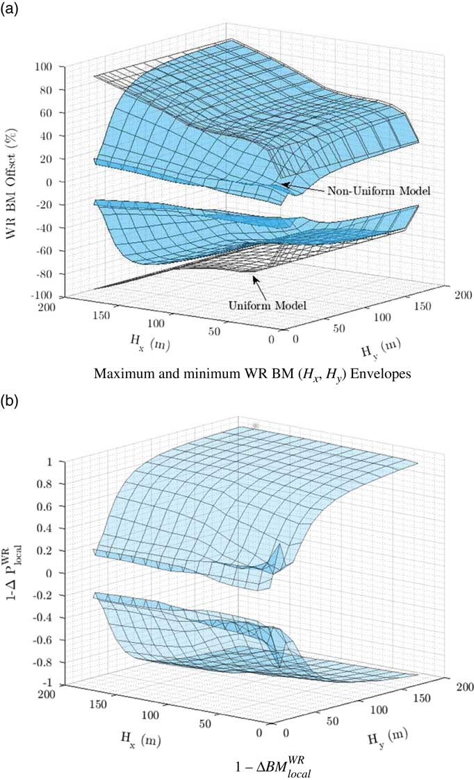
Figure 9 Gust loads envelope for WR BM and model normalised difference (FC 5 LC 1 set-up).
As the normalised difference illustrated in Fig. 9(b) lies well between 0 and 1 for the entire spectrum of gust gradients, it could be concluded that the addition of the spanwise variation function has not introduced disruptive modifications to structural loading maximum or minimum values when compared to the conventional model. In fact, in the region of lower gust gradients in the (H x ,H y ) plane, the difference between the two models is significant, which could highlight potential over-engineering or conservative practices. But as only gust induced fuselage angle-of-attack were kept identical between conventional and non-uniform model for similar gust gradients (not vertical acceleration), it can be argued that both models do not effectively lead to an equivalent worst case gust. As models were in part historically derived from vertical acceleration measurements, it would be more relevant to compare structural loads induced by gusts of similar load factors n g .
By examining the contours of both vertical acceleration n g and any structural wing root IQ, a number of equivalent conventional gusts can be found for any non-uniform gust encounter. The example of wing root bending moment is given in Fig. 10, where both maximum of wing root bending moment and n g values reached during the bidirectional loads process are given for a specific flight case. With the conventional model equivalent to the higher H y gradients given in the far right of the contour plot, an infinite number of equivalent non-uniform gusts can be found to reach similar wing root loading when following the maximum WR BM contour (Fig. 10).
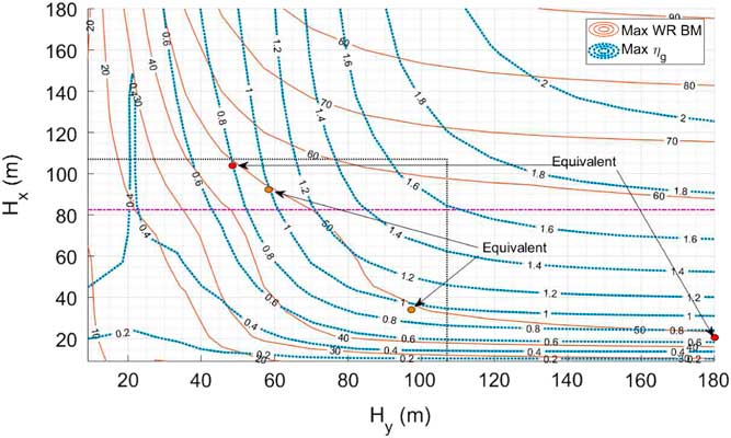
Figure 10 Wing root BM and fuselage n g maximum contours for various gust gradients (FC 5 LC 1 set-up).
On the other hand, these do not lead to equivalent vertical load n
g
for the entire path. Therefore, comparable gust measurements based on n
g
do not lead to similar loadings with the non-uniform gusts. By overlaying both metrics, specific (H
x
,H
y
) couples can be found where equivalent wing root loading is obtained for similar maximum n
g
as shown in the plot (orange dot). It is also possible to find equivalent points between the conventional model and the non-uniform model (red dot). Hence, it is possible to induce similar maximum wing root loading and n
g
with different gust velocity fields (but the same maximum angle-of-attack due to gust at the fuselage) when investigating a single structural IQ such as bending moment in this example. Furthermore, the effect of H
y
on wing root loading for a constant n
g
varies with the specified value of n
g
and considered chordwise gradient. In the (H
x
,H
y
) plane area where
 $$H_{x} \leq 100$$
and
$$H_{x} \leq 100$$
and
 $$H_{y} \leq 100$$
and for a given n
g
, reducing H
y
leads to an initial reduction in structural load before increasing back as H
x
increases to following the iso n
g
line. In other parts of the (H
x
,H
y
) plane, including the H
y
gradient to match vertical load can lead to higher wing root loading maximum, specifically for high H
x
gradients (above certification recommendations of 107 m). Similar trends were identified for all flight and loading cases. The impact of aircraft loading on the airframe bending moment loading and vertical accelerations are given in Fig. 11(a) and (b). A significant loading difference is noticed in the LC 2 (as expected for a heavy landing configuration) for all gust gradient co-ordinates. Smaller changes to the load factor n
g
are also registered. Otherwise, the overall trend of the contour is very similar, leading to similar conclusions in all loading and flight conditions.
$$H_{y} \leq 100$$
and for a given n
g
, reducing H
y
leads to an initial reduction in structural load before increasing back as H
x
increases to following the iso n
g
line. In other parts of the (H
x
,H
y
) plane, including the H
y
gradient to match vertical load can lead to higher wing root loading maximum, specifically for high H
x
gradients (above certification recommendations of 107 m). Similar trends were identified for all flight and loading cases. The impact of aircraft loading on the airframe bending moment loading and vertical accelerations are given in Fig. 11(a) and (b). A significant loading difference is noticed in the LC 2 (as expected for a heavy landing configuration) for all gust gradient co-ordinates. Smaller changes to the load factor n
g
are also registered. Otherwise, the overall trend of the contour is very similar, leading to similar conclusions in all loading and flight conditions.
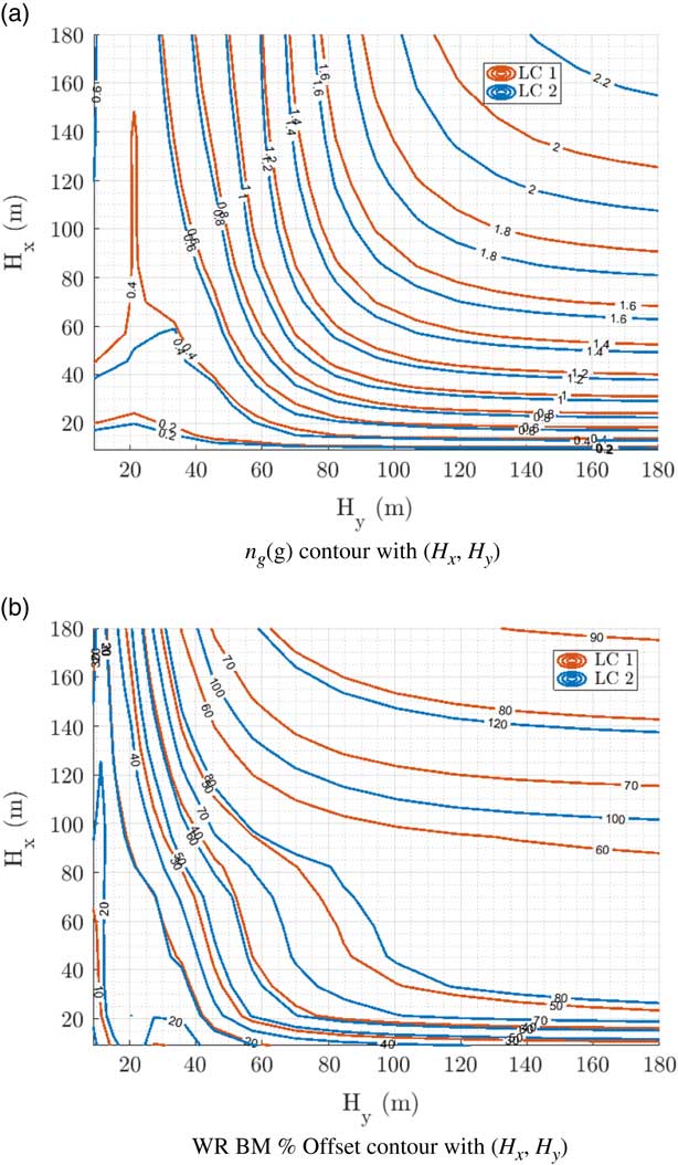
Figure 11 Fuselage n g and WR BM maximum contours comparison for two loading cases (FC 5 set-up).
This could mean that conventional loads practices lead to lower maximum critical loads by assuming uniform models, as a non-uniform model leads to worse loads in specific gust specifications. The extension of the uniform model with spanwise variation introduced new worst case scenarios for wing root bending moment for gusts with matching maximum load factor n g measurements. Despite being minor overshoot when confined to the 107 m certification gradient limitation, this could potentially lead to uniform models becoming unsuitable for worst case loading identification and loads alleviation investigations. This has also only been verified for the aircraft configuration presented herein and could potentially be different for a design employing HARW or any other disruptive design.
5.2 Impact of H y on aircraft time-correlated gust loads
Extreme loading is not the only concern when investigating structural loads and flight dynamics as a result of discrete gust encounters. Given the scope of this study, it is also relevant to investigate the effect of the additional gradient H y on loads time histories throughout the entire gust encounter and recovery scenario. Therefore, time histories were used to compare all different H y gust gradient results for given H x , direction and FC sets. An illustrative comparison of H y gradients impact on loads for a given H x =82 m upward vertical gust (purple line in Fig. 10) is used in this section. Wing root bending moment (Fig. 12(a)), torsion moment (Fig. 12(b)), vertical load factor n g (Fig. 12(d)) and pitch angle θ (Fig. 12(c)) are monitored throughout the entire simulation.
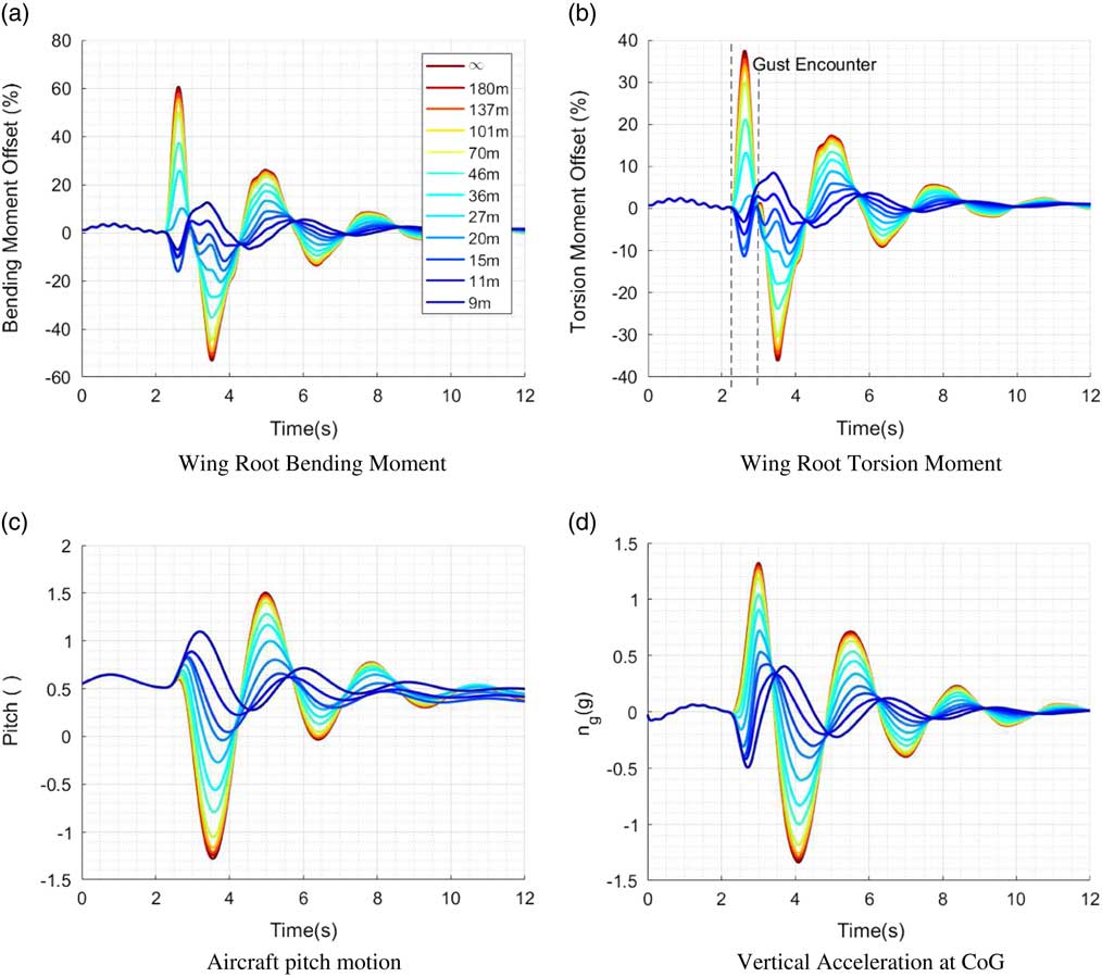
Figure 12 Effect of H y for H x =82 m on wing root and fuselage IQs (FC 5 LC 1 upward gust set-up).
Gust-induced loading (initial peak) as well as the loading due to aircraft’s inherent restoring motion (secondary peak and onward) is clearly visible in the loading history given in Fig. 12. In this example, the pitch-induced loading (secondary peak) clearly defines the minimum loading for torsion, bending moment and shear force. In the symmetric downward gust scenario, it defines the maximum loading values. With increasing values of H
x
, the amplitude of pitch and heave induced loading overtakes the initial peak. Therefore, when analysing both upward and downward gusts together at a given flight condition, extreme loads can occur during the aircraft pitch and heave oscillation after and not during the gust encounter for the higher end of H
x
. This is confirmed by the break in surface gradient in Fig. 9(a). The value of H
x
at which pitch induced loading overtakes the gust induced loading differs among IQs, flight and loading cases. In these conditions, the limit has been identified at
 $$H_{x} {\gtrsim}90\,{\rm m}$$
for root bending and
$$H_{x} {\gtrsim}90\,{\rm m}$$
for root bending and
 $$H_{x} {\gtrsim}80\,{\rm m}$$
for root torsion moment. This does not apply to the lower H
y
spectrum, where despite pitch and vertical accelerations peaks, structural loads do not follow the conventional oscillation trend, and is clearly visible in the above-mentioned envelope plots (Fig. 9(a) and (b)).
$$H_{x} {\gtrsim}80\,{\rm m}$$
for root torsion moment. This does not apply to the lower H
y
spectrum, where despite pitch and vertical accelerations peaks, structural loads do not follow the conventional oscillation trend, and is clearly visible in the above-mentioned envelope plots (Fig. 9(a) and (b)).
Note that H y gradients below wing semi-span lead to gust induced loading of opposite direction as velocity direction flips along the wingspan. This means that a conventional uniform gust with matching initial acceleration maxima would be of opposite direction, despite both models matching fuselage gust angle-of-attack values in the present settings. Hence, structural loading time histories, similar to maximum loading, differ drastically with changing H y . Furthermore, oscillations for both root torsion and bending moments appear at approximately 2.4 Hz after the gust encounter. This frequency matches that of the second wing bending mode of the aircraft which is not as severely excited by the uniform model.
For values similar to aircraft semi-span (27.4 m in this example), the wing root bending and torsion moments are only slightly modified during the gust encounter (seen in Fig. 12(a) and (b)) despite having significant n g and pitch motion induced by the gust (seen in Fig. 12(c) and (d)). As H y increases to the higher end of the spectrum, all quantities converge to the conventional trend. Maximum loading and worst case gusts occur with the conventional model for all H x gradients, gust directions, aircraft loading and flight conditions included in this simulation set. This is verified for the given f y intensity distribution and was expected because the overall gust velocity integral during the encounter is lower in the non-uniform model.
With the apparition of lags and time delays with H y in both wing root bending and torsion moments, it must be verified that the non-uniform model does not introduce radically different torsion/bending paths to the conventional model. In other words, no radical phase delay is introduced. An example of the widely used bending/torsion correlated plot, or Convex Hull plot is given in Fig. 13. Once again, the effect of H y on maximal loads amplitude is clear, where loads due to larger H y gradients clearly exceed those obtained with the lower end of the spectrum. The high collinearity of the linear structural model is highlighted in the diagram, torsion and bending values being highly linked in the gust encounter scenario due to the aircraft structural model properties. Despite being negligible on the overall maximum loading, a small deviation from the quasi-linear correlation is induced for H y between 15 m and 27 m during the first seconds of the encounter, highlighting the impact of the difference in second wing bending moment excitation. When comparing all gust gradient combinations, gust directions, flight conditions and aircraft loading cases, H y does not lead to any other significant changes in coupled bending/torsion envelopes, and, therefore, does not introduce more major phase delays between the two quantities.
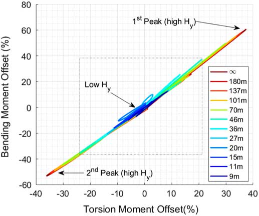
Figure 13 Effect of H y for H x =82 m on correlated bending/torsion moment path (FC 5 LC 1 upward gust set-up).
Overall, the addition of the spanwise variation function has introduced major trend modifications to structural loading time histories for low H y values. Small phase shifts as well as oscillations linked to wing flexibility have been encountered in specific cases. Lower gust gradients have also led to inverted peak magnitudes. But maximum loading amplitude is clearly still defined by the uniform model for all loading and flight dynamic IQs. Maximum bending and torsion moment path contour have also seen very little modifications. Therefore, when comparing similar H x gust gradients, the uniform model still appears as the most critical. Despite this, it would be relevant to compare the time histories of matching n g similar to what was done before and investigate the implications of the non-uniform loading on the time histories, and is included in further development plans of the process.
5.3 Non-uniform discrete models and loads alleviation
Active loads alleviation systems ideally require predictive actuation for best efficiency. Ideally, predictive local angle-of-attack measurements would greatly improve loads alleviation strategies. Actuation systems require predictive measurements to be efficient, as actuation is not instantaneous.
But currently, loads alleviation relies on angle-of-attack measured at the nose of the aircraft as well as the load factor n g measured from the fuselage and conventional systems such as spoilers or ailerons are distributed along the wings to ensure efficient off-load. The wing lag in penetrating the gust compared to the nose helps in pre-emptive surface actuation. If wing-tip systems or outboard ailerons are used, their physical positioning implies that the effective disturbance could be drastically different to that measured at the nose of the aircraft. This is particularly true for low H y gradients. Outer wing gust velocities being of opposite signs to that of the fuselage for the lower H y gradients system deployment could potentially be detrimental or dangerous if loads alleviation is achieved by effective angle-of-attack modifications such as ailerons.
In this section, the authors have investigated a possibility to consider both n g and α b as a correlated pair, to differentiate gusts of various H y , which would in turn require different off-load control strategies. This could ideally be possible once a better understanding of the relation between α b and n g for a uniform and non-uniform model is achieved (through the analysis of a sufficiently large database of spanwise distribution functions). Corrected loads alleviation strategies could then be developed to account for non-uniform gusts.
Hence, the effect of H y on the coupled metrics is analysed. A coupled α b (n g ) path, or phase plot, is given Fig. 14(a), next to the WR BM(n g ) path given in Fig. 14(b). α b accounts for pitch and gust-induced modifications, corresponding to on-board instrument measurements. Changes in H y clearly leads to variations in the α b (n g ) path, shifting n g to the opposite sign as H y decreases. The amplitude and trend of α b is also modified with pitching and vertical heave motion transferred to the aircraft. Therefore, a difference in gust shape can be identified solely based on coupled measurements of α b and n g quite quickly into the encounter (within the first 1/10th of a second). Symmetric behaviour is obtained for a downward gust. During build up to the initial α b peak (which occurs roughly at the same time for all H y gradients), the value of n g values can be used to assess the dominant motion of the aircraft and therefore correct for the alleviation strategy.
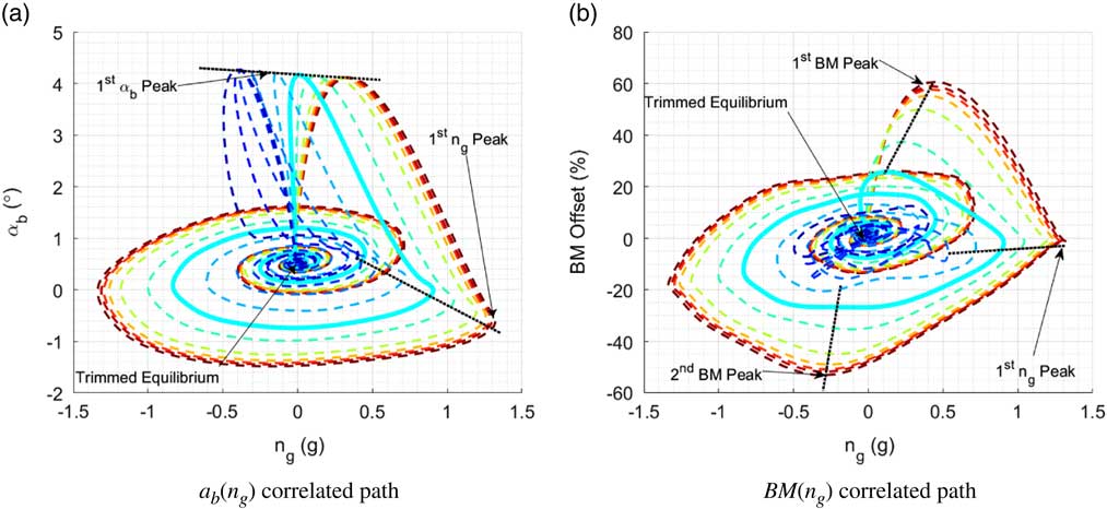
Figure 14 Effect of H y on wing root and fuselage IQ correlated paths (FC 5 LC 1 upward gust set-up).
Therefore, if perfected to recognise non-uniform loading, the loads alleviation system could respond according to best applicable strategy (loads alleviation, passenger comfort, etc.). In Fig. 14(a), one can easily see the phase shift between the angle-of-attack, reaching nearly identical maximum values, and the simultaneous load factor, for various H
y
. A gradient H
y
of 36 m is highlighted in cyan as an example. Using Fig. 14(a) and previous times histories and plots, it can be seen that for that gradient, wing root loading reaches
 $$\,\pm30\,\%\,$$
offset relative to trim, corresponding to a uniform model vertical load factor (seen from Fig. 10 of approximately 0.2 g). In the non-uniform case, the maximum vertical load factor is much higher, at 0.9 g during the first
$$\,\pm30\,\%\,$$
offset relative to trim, corresponding to a uniform model vertical load factor (seen from Fig. 10 of approximately 0.2 g). In the non-uniform case, the maximum vertical load factor is much higher, at 0.9 g during the first
 $$n_{g} $$
peak. This corresponds to a 45% BM loading in the conventional model, which could in turn lead to an excess load alleviation strategy, applied at the wrong time. If parametrised, the phase difference between the two metrics, specifically during the gust encounter, could ideally be used to improve load alleviation strategies specifically during the gust encounter with only fuselage angle-of-attack and load factor measurements. This analysis can be made in all test cases. Hence, for any given H
x
gradient, gust direction, FC and LC of the tested aircraft and f
y
distribution function, load alleviation during gust loads application to the aircraft could lead to drastically different performances and results depending on H
y
values, specifically for the lower end of the spectrum, below wing semi-span.
$$n_{g} $$
peak. This corresponds to a 45% BM loading in the conventional model, which could in turn lead to an excess load alleviation strategy, applied at the wrong time. If parametrised, the phase difference between the two metrics, specifically during the gust encounter, could ideally be used to improve load alleviation strategies specifically during the gust encounter with only fuselage angle-of-attack and load factor measurements. This analysis can be made in all test cases. Hence, for any given H
x
gradient, gust direction, FC and LC of the tested aircraft and f
y
distribution function, load alleviation during gust loads application to the aircraft could lead to drastically different performances and results depending on H
y
values, specifically for the lower end of the spectrum, below wing semi-span.
All points of the aircraft, despite lags and offsets due to flexibility that can be accounted for, share common flight dynamics during manoeuvre. This can easily be seen through all time history plots, and phase plots presented above, as all metrics converge to similar trends and values with time during the restoring pitch and heave motion. Therefore, when loads are generated by aircraft pitching and flight dynamics in the gust recovery phase, centralised measurements can be used to apply spanwise distributed loads alleviation strategies similar to what is conventionally done in manoeuvre loads alleviation.
5.4 Intensity tuning method comparison
As described in the framework set-up, a new intensity tuning or scaling method was derived based on an isotropic model assumption. Both gradients are now used to define the maximum gust intensity. This naturally had some drastic effects on the gust loads. Similar to what was introduced earlier, Fig. 15(a) and (b) represents the new loading envelope encountered during the gust.
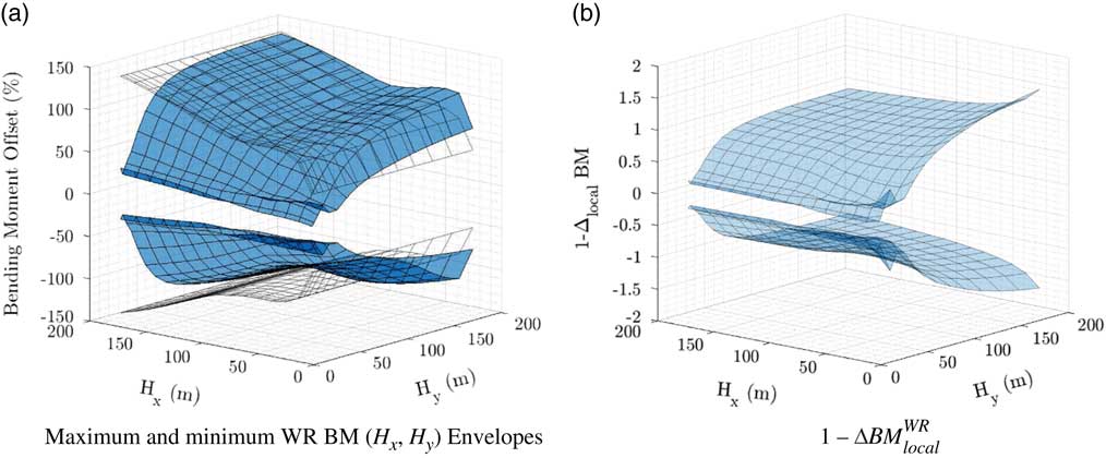
Figure 15 Gust loads envelope for WR BM and model normalised difference with multidimensional intensity scaling (FC 5 LC 1 set-up).
This new scaling approach clearly leads to more intense loading in some regions of the (H
x
,H
y
) plane, more specifically where
 $$H_{y} \,\gg\,H_{x} $$
. This corresponds to regions where the spanwise gust gradient is used to scale the gust intensity. It is clear from the surface plots that the non-uniform model now exceeds the uniform model for specific gust gradients. Nevertheless, a comparison based on the global normalised difference shows that maximum loading is still achieved with the uniform model when comparing all gust gradient couples.
$$H_{y} \,\gg\,H_{x} $$
. This corresponds to regions where the spanwise gust gradient is used to scale the gust intensity. It is clear from the surface plots that the non-uniform model now exceeds the uniform model for specific gust gradients. Nevertheless, a comparison based on the global normalised difference shows that maximum loading is still achieved with the uniform model when comparing all gust gradient couples.
Once again, a comparison for matching vertical load factor n g must be made. Similar to what was obtained with the previous model, it is possible to find equivalent gusts in terms of n g that lead to higher bending moment or torsion moment at the aircraft wing root. Furthermore, the trend of all metrics envelope has significantly changed, as shown in the contours of Fig. 16(a) and (b) which compare results of similar flight conditions and loading for the two intensity scaling methods. By overlaying both metrics, a similar analysis to that which was made in Section 5.1 can be made: greater loading can be achieved with the non-uniform model for a given n g . In terms of time history trends (time-correlated), results are very similar between the scaling methods. Only the maximal amplitudes vary significantly.
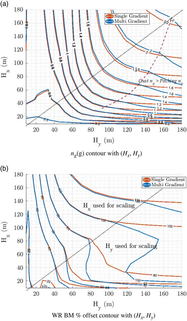
Figure 16 Fuselage n g and WR BM maximum contours comparison for two tuning methods (FC 5 LC 2 set-up).
It can be seen from this brief comparison of gust intensity scaling methods that an even greater difference has been introduced over a significant area of the gust gradient plane. The worst case gust scenario, in the case of a large conventional aircraft, is reached in the non-uniform model for a non-negligible area of the (H x ,H y ) plane when the multi-gradient tuning method is used.
Results have focused exclusively on wing root quantities in this paper. But distributed loading is also influenced by H y . Further investigations focusing on the distributed loads along the wing, and not exclusively wing root, could also lead to interesting conclusions regarding H y impact on design loads.
6.0 CONCLUSIONS
Within this paper, the authors have introduced a spanwise non-uniform discrete gust model, inspired by recommendations made for HALE UAV design( 34 ), within a large civil aircraft loads calculation process. This is justified with an historical review of past and current industrial practices. Hence, a time domain simulation framework was modified to allow for spanwise non-uniform discrete gust encounter simulations. Multiple flight conditions and mass cases of a generic large aircraft were used as an example to illustrate the impact of such modifications on airframe loads. Using the isotropic characteristic of the atmosphere, the spanwise distribution function was derived similar to the original certification model. Overall, gust fields were derived to keep the gust induced angle-of-attack at the fuselage similar between the two models, regardless of the spanwise gradient value.
The non-uniform gust model caused changes to both wing root loading envelopes and time-correlated loads. When using similar gust gradients and conventional intensity tuning method, the critical loads envelope was obtained with the uniform gust model for all mass cases and flight conditions. In fact, the maximum envelope is defined by the heavy mass case at sea level. The use of the multi gradient intensity scaling method caused higher loads in specific areas of the gust gradient plane. Localised overshoots in maximum uncorrelated loads and changes in time-correlated histories of all wing root IQs were highlighted. The maximum load factor did not display similar variations, which leads to higher airframe loads for a given load factor in the non-uniform model. Therefore, a shortfall in critical gust loads analysis has been identified for the conventional model, as the non-uniform model henceforth exceeds the certification loadings for particular gust gradients. Despite selecting a spanwise distribution function so as to match angle-of-attack at the fuselage regardless of H y , the vertical load n g differed. The certification model was derived from both vertical acceleration and angle-of-attack measurements and empirically scaled to be applied to all aircraft. Hence, a comparison based on matching n g rather than gust gradients is more suitable. By matching vertical acceleration measurements between the uniform and non-uniform gust results, higher airframe loads are obtained in specific areas of the (H x ,H y ) plane with the non-uniform gust for all test configurations. Hence, the spanwise uniform model can be seen as unsuitable to capture the critical loading case, even in the case of a conventional large flexible aircraft. Concerns regarding current investigations in loads alleviation strategies were also raised. The use of centralised vertical acceleration or angle-of-attack measurement has been identified as possibly insufficient to ensure effective off-load with distributed alleviation systems in the event of non-uniform loading.
A major limitation to the present conclusions is the lack of atmospheric measurements and experimental data to validate a realistic non-uniform model, and the specific assumption made of f y . If the presented distribution function f y was to be identified as realistically plausible, these results would challenge the uniform models’ applicability to large flexible airframes. It would also impact methods used to apply gust reconstruction( Reference Simeone, Rendall and Da Ronch 54 ), rendering the process more complex and challenging.
Overall, this paper has highlighted a potential shortfall of the conventional discrete gust model to capture worst case structural loading compared to a non-uniform model. To consolidate these results, further investigations must be carried out so as to broaden the applicability of these findings. The inclusion of more flight conditions, loading scenarios, more complex velocity directions could help identify new worst non-uniform gust loading cases more precisely. Furthermore, investigating round-the-clock gusts could potentially highlight other gust directions and spanwise distribution to be critical to the process. Other aircraft geometries and wing structural properties should also be considered, such as HARW concepts. This will allow the assessment of the applicability of the conventional gust model to newer and more disruptive realistic aircraft concepts. The monitoring of distributed loading may also lead to interesting results, as only wing root IQs were investigated in this paper.
APPENDIX
Figure A1. Sample of AX-1 mode shapes (loading of approximately 80% MTOW).