2.1. Ordinary single-layered Ornstein–Uhlenbeck process

Standard arguments developed in turbulence phenomenology (Tennekes & Lumley Reference Tennekes and Lumley1972) lead to the consideration of, as a stochastic model for velocity of Lagrangian tracers, the OU process. In particular, such a process reaches a statistically stationary regime in which variance is finite and exponentially correlated. Let us denote such a process by $v_1(t)$, and define it as the unique stationary solution of the following stochastic differential equation, also called Langevin equation,

(2.1)\begin{equation} {\rm d} v_1(t) ={-}\frac{1}{T}v_1(t) \,{\rm d} t + \sqrt{q}W({\rm d} t), \end{equation}

where $T$ is the turbulence (large) turnover time, $W(t)$ is a Wiener process and $W({\rm d} t)$ its infinitesimal increment over ${\rm d} t$ (i.e. independent instances of a Gaussian random variable, zero average and of variance ${\rm d} t$). It obeys the following rule of calculation (cf. Nualart Reference Nualart2000): any appropriate deterministic functions $f$ and $g$, which follow particular integrability conditions such that,

(2.2)\begin{equation} \left\langle \int_\mathcal{A} f(t)W({\rm d} t)\right\rangle=0, \end{equation}

and

(2.3)\begin{equation} \left\langle \int_\mathcal{A} f(t)W({\rm d} t)\int_\mathcal{B} g(t)W({\rm d} t)\right\rangle=\int_{\mathcal{A}\cap \mathcal{B}} f(t)g(t)\,{\rm d} t, \end{equation}

where $\langle \cdot \rangle$ stands for ensemble average, and $\mathcal {A}\cap \mathcal {B}$ is the intersection of the two ensembles $\mathcal {A}$ and $\mathcal {B}$.

The unique statistically stationary solution of the stochastic differential equation (SDE) provided in (2.1) can be written conveniently as

(2.4)\begin{equation} v_1(t) = \sqrt{q}\int_{-\infty}^{t} {\rm e}^{-(t-t')/T} W({\rm d} t'). \end{equation}

Since $v_1$ is defined as a linear operation on the Gaussian white noise $W({\rm d} t)$, it is Gaussian itself. Following the rules given in (2.2) and (2.3), it is thus fully characterized by its average and correlation function. In particular, $v_1$ is a zero-average process, i.e. $\langle v_1 \rangle =0$, and is correlated as

(2.5)\begin{align} \mathcal{C}_{v_1}(t_1-t_2)\equiv \langle v_1(t_1)v_1(t_2) \rangle = q\int_{-\infty}^{min (t_1,t_2)} \exp({-(t_1+t_2-2t)/T})\, {\rm d} t = \frac{qT}{2} {\rm e}^{-|t_1-t_2|/T}. \end{align}

Notice that $v_1$ is a finite-variance process $\langle v_1^2\rangle = qT/2$ (consider the value of the correlation function (2.5) at equal times, $t_1=t_2$), and behaves at small scales as a Brownian motion, as is required by the dimensional arguments developed in the standard phenomenology of turbulence at infinite Reynolds number (Tennekes & Lumley Reference Tennekes and Lumley1972). To see this, define the velocity increment as

(2.6)\begin{equation} \delta_\tau v_1(t) \equiv v_1(t+\tau)-v_1(t), \end{equation}

and notice that

(2.7)\begin{equation} \left\langle \left(\delta_\tau v_1(t)\right)^2 \right\rangle = 2\left[\left\langle v_1^2\right\rangle-\mathcal{C}_{v_1}(\tau)\right]\mathop{\sim}\limits_{\tau\rightarrow 0} q|\tau|. \end{equation}

The scaling behaviour given in (2.7) is typical of non-differentiable processes. Hence, the respective acceleration process $a_1(t) \equiv {\rm d} v_1/{\rm d} t$ is ill-defined (actually it is a random distribution). To circumvent this pathological behaviour, Sawford (Reference Sawford1991) has proposed introducing the dissipative Kolmogorov time scale $\tau _\eta$, which will be discussed in the following section.

2.2. Embedded Ornstein–Uhlenbeck processes

2.2.1. Two layers: the Sawford model

Here, we follow the approach developed by Sawford (Reference Sawford1991). We consider the following embedded OU process $v_2(t)$:

(2.8)\begin{equation} \frac{{\rm d} v_2}{{\rm d} t} ={-}\frac{1}{T}v_2(t)+ f_1(t), \end{equation}

where $f_1(t)$ in an external random force that obeys itself an ordinary OU process, as discussed in § 2.1, but exponentially correlated over the small time scale $\tau _\eta$. It is thus defined as the unique solution of the following SDE

(2.9)\begin{equation} {\rm d} f_1(t) ={-}\frac{1}{\tau_\eta}f_1(t) \,{\rm d} t + \sqrt{q}W({\rm d} t). \end{equation}

Hence, it is a zero-average Gaussian process, and its correlation function is given by

(2.10)\begin{equation} \mathcal{C}_{f_1}(\tau)\equiv \langle \, f_1(t)f_1(t+\tau) \rangle = \frac{q\tau_\eta}{2} {\rm e}^{-|\tau|/\tau_\eta}. \end{equation}

The unique statistically stationary solution of (2.8) is once again given by

\[ v_2(t) = \int_{-\infty}^{t} {\rm e}^{-(t-t')/T} f_1(t')\,{\rm d} t', \]

showing that $v_2$ is a zero-average Gaussian process, and correlated as

(2.11)\begin{equation} \mathcal{C}_{v_2}(\tau)\equiv \langle v_2(t)v_2(t+\tau) \rangle = \int_{-\infty}^{t} \int_{-\infty}^{t+\tau} \exp({-(2t+\tau-t_1-t_2)/T})\mathcal{C}_{f_1}(t_1-t_2)\,{\rm d} t_1\, {\rm d} t_2. \end{equation}

Assuming without loss of generality $\tau \ge 0$ (recall that the correlation function of a statistically stationary process is an even function of its argument), splitting the integral entering in (2.11) over the dummy variable $t_2$ into the two sets $[-\infty ,t]$ and $[t,t+\tau ]$, and performing the remaining explicit double integral, we obtain the following expression:

(2.12)\begin{equation} \mathcal{C}_{v_2}(\tau)= \frac{q \tau_{\eta}^2 T^2}{2(T^2-\tau_{\eta}^2)}\left[T {\rm e}^{-|\tau|/T} - \tau_{\eta}{\rm e}^{-|\tau|/\tau_{\eta}}\right], \end{equation}

which is in agreement with the formula given by Sawford (Reference Sawford1991).

The respective acceleration process $a_2(t)\equiv {\rm d} v_2(t)/{\rm d} t$, obtained from (2.8), is accordingly a zero-average Gaussian process, and its correlation function is given by

(2.13)\begin{align} \mathcal{C}_{a_2}(\tau)&\equiv \langle a_2(t)a_2(t+\tau) \rangle\nonumber\\ &={-}\frac{{\rm d}^2}{{\rm d}\tau^2} \langle v_2(t)v_2(t+\tau) \rangle= \frac{q \tau_{\eta}^2 T^2}{2(T^2-\tau_{\eta}^2)}\left[ -\frac{1}{T}{\rm e}^{-|\tau|/T} + \frac{1}{\tau_{\eta}}{\rm e}^{-|\tau|/\tau_{\eta}}\right]. \end{align}

Notice that the function $\mathcal {C}_{v_2}$ (2.12) is indeed twice differentiable at the origin, contrary to the function $\mathcal {C}_{v_1}$ (2.5), such that $a_2$ has finite variance given by $\mathcal {C}_{a_2}(0)$ (2.13).

2.2.2. Generalization to $n$ layers

By iterating the aforementioned procedure, we can consider similarly $n$ additional layers instead of a single one, as proposed in the embedded Ornstein–Uhlenbeck process (2.8) by Sawford. Here, acceleration is a well-defined random process and so are the velocity derivatives of order $n$. Once again, these additional layers will eventually be modelled as OU processes. A similar type of procedure has been adopted in Arratia, Cabana & Cabana (Reference Arratia, Cabana and Cabana2014) in a different context. The obtained embedded structure is defined using a set of $n$ coupled stochastic ordinary differential equations (ODEs), with $n\ge 2$, that reads

(2.14)\begin{gather} \frac{{\rm d} v_n}{{\rm d} t} ={-}\frac{1}{T}v_n(t)+ f_{n-1}(t), \end{gather}

(2.15)\begin{gather}\frac{{\rm d} f_{n-1}}{{\rm d} t} ={-}\frac{1}{\tau_{\eta}}f_{n-1}(t)+ f_{n-2}(t), \end{gather}

(2.16)\begin{gather}\cdots \end{gather}

(2.17)\begin{gather}\frac{{\rm d} f_{2}}{{\rm d} t} ={-}\frac{1}{\tau_{\eta}}f_{2}(t)+ f_{1}(t), \end{gather}

(2.18)\begin{gather}{\rm d} f_1 ={-}\frac{1}{\tau_\eta}f_1(t) \,{\rm d} t + \sqrt{q_{(n)}}W({\rm d} t). \end{gather}

The remaining free parameter $q_{(n)}$ can be eventually chosen such that

(2.19)\begin{equation} \langle v_n^2\rangle = \sigma^2, \end{equation}

independently of $\tau _\eta$ and/or the number of layers $n$, as is required by the standard phenomenology of Lagrangian turbulence (Tennekes & Lumley Reference Tennekes and Lumley1972).

We present in Proposition A.1 the explicit computation of the correlation functions of velocity $v_n$ and the respective acceleration $a_n$ in the statistically stationary regime, obtained from the set of (2.14)–(2.18) as $t\to \infty$. Their expressions are especially simple in the spectral domain, and read, considering $n\ge 2$ to ensure that acceleration is a well-defined process,

(2.20)\begin{equation} \mathcal{C}_{v_n}(\tau) = q_{(n)}\int_{\mathbb{R}}{\rm e}^{2\, \textrm{i}{\rm \pi} \omega\tau}\frac{T^2}{1+4{\rm \pi}^2T^2\omega^2}\left[\frac{\tau_\eta^{2}}{1+4{\rm \pi}^2 \tau_\eta^2\omega^2}\right]^{n-1}\, {\rm d} \omega, \end{equation}

and

(2.21)\begin{equation} \mathcal{C}_{a_n}(\tau)= q_{(n)}\int_{\mathbb{R}}4{\rm \pi}^2\omega^2 {\rm e}^{2\, \textrm{i}{\rm \pi} \omega\tau}\frac{T^2}{1+4{\rm \pi}^2T^2\omega^2}\left[\frac{\tau_\eta^{2}}{1+4{\rm \pi}^2 \tau_\eta^2\omega^2}\right]^{n-1}\, {\rm d} \omega, \end{equation}

where the multiplicative factor $q_{(n)}$ (defined in (A 6)) enforces the prescribed value of velocity variance (2.19). Let us notice that taking $n=2$ layers, the respective correlation of the process $v_2$ coincides with the one proposed in Sawford (Reference Sawford1991), as recalled in § 2.2.1.

It is interesting to consider the limiting process $v$ or $a$ when the number of layers $n$ goes towards infinity from a physical point of view, which would give an example of a causal infinitely differentiable process, if such a process exists. It is indeed possible to show rigorously that the correlation function of $v_n$ (2.20) loses its dependence on the time scale $\tau$. We then have $\mathcal {C}_{v_n}(\tau )\rightarrow \sigma ^2$ for any $\tau \ge 0$ as $n\rightarrow \infty$. Thus, asymptotically, the limiting process does not decorrelate, which is at odds with the expected behaviour. We will see in the following § 2.3 that by considering the re-scaled dissipative time scale $\tau _\eta /\sqrt {n-1}$ instead of $\tau _\eta$, the system of equations will converge towards a proper process with an appropriate correlation function as $n\rightarrow \infty$.

2.3. Towards an infinitely differentiable causal process

Consider the following system of embedded differential equations:

(2.22)\begin{gather} \frac{{\rm d} v_n}{{\rm d} t} ={-}\frac{1}{T}v_n(t)+ f_{n-1}(t), \end{gather}

(2.23)\begin{gather}\frac{{\rm d} f_{n-1}}{{\rm d} t} ={-}\frac{\sqrt{n-1}}{\tau_{\eta}}f_{n-1}(t)+ f_{n-2}(t), \end{gather}

(2.24)\begin{gather}\cdots \end{gather}

(2.25)\begin{gather}\frac{{\rm d} f_{2}}{{\rm d} t} ={-}\frac{\sqrt{n-1}}{\tau_{\eta}}f_{2}(t)+ f_{1}(t), \end{gather}

(2.26)\begin{gather}{\rm d} f_1 ={-}\frac{\sqrt{n-1}}{\tau_\eta}f_1(t) \,{\rm d} t + \sqrt{\alpha_{n}}W({\rm d} t), \end{gather}

with

(2.27)\begin{gather} \alpha_n=\left(\frac{n-1}{\tau_\eta^2}\right)^{n-1} \frac{2\sigma^2{\rm e}^{-\tau_\eta^2/T^2}}{T{\rm erfc}\left(\tau_\eta/T\right)}, \end{gather}

where we have introduced the error function $\textrm {erf}(t) =(2/\sqrt {{\rm \pi} })\int _0^t{\rm e}^{-s^2}\, {\rm d} s$, and its respective complementary $\textrm {erfc}(t)=1-\textrm {erf}(t)$. The chosen white noise weight $\alpha _n$ (2.27) ensures that the variance of the limiting process $v$ is finite with $\langle v^2\rangle =\sigma ^2$.

We summarize and derive in appendix A (see Proposition A.2) the statistical properties of the unique statistically stationary solution of the set of embedded differential (2.22)–(2.26). In particular, the velocity correlation function now reads

(2.28)\begin{equation} \mathcal{C}_{v_n}(\tau) = \frac{2\sigma^2{\rm e}^{-\tau_\eta^2/T^2}}{T{\rm erfc}\left(\tau_\eta/T\right)}\int_{\mathbb{R}}{\rm e}^{2\, \textrm{i}{\rm \pi} \omega\tau}\frac{T^2}{1+4{\rm \pi}^2T^2\omega^2}\left[\frac{1}{1+ \dfrac{4{\rm \pi}^2\tau_\eta^2\omega^2}{n-1}}\right]^{n-1}\, {\rm d} \omega. \end{equation}

Whereas the function provided in (2.20) does not converge towards a correlation function of a well-behaved stochastic process as the number of layers goes to infinity, (2.28) does. In other words, through iteration of the set of embedded differential equations, (2.22)–(2.26), over an infinite number of layers $n\rightarrow \infty$, we obtain an infinitely differentiable and causal Gaussian process, in which the velocity correlation function reads, in the stationary regime,

(2.29)\begin{equation} \mathcal{C}_{v}(\tau)= \sigma^2\frac{{\rm e}^{-|\tau|/T}}{2{\rm erfc}(\tau_\eta/T)}\left[1+\textrm{erf} \left(\frac{|\tau|}{2\tau_\eta}-\frac{\tau_\eta}{T}\right)+ {\rm e}^{2|\tau|/T}{\rm erfc}\left(\frac{|\tau|}{2\tau_\eta}+\frac{\tau_\eta}{T}\right)\right]. \end{equation}

Let us notice that indeed $\mathcal {C}_{v}(0)=\langle v^2\rangle =\sigma ^2$. Furthermore, taking the second derivatives of (2.29) and multiplying by the factor $-1/2$, we obtain the respective acceleration correlation function

(2.30)\begin{align} \mathcal{C}_{a}(\tau)&= \frac{\sigma^2}{2T^2{\rm erfc}(\tau_\eta/T)}\left[\frac{2T}{\tau_\eta\sqrt{\rm \pi}} \exp\left({-\left( \frac{\tau^2}{4\tau_\eta^2}+\frac{\tau_\eta^2}{T^2}\right)}\right)-{\rm e}^{-|\tau|/T}\left(1+ \textrm{erf}\left(\frac{|\tau|}{2\tau_\eta}-\frac{\tau_\eta}{T}\right)\right)\right. \nonumber\\ &\quad\left.-{\rm e}^{|\tau|/T}{\rm erfc}\left(\frac{|\tau|}{2\tau_\eta}+\frac{\tau_\eta}{T}\right)\right]. \end{align}

2.4. A first numerical illustration

A first numerical illustration is proposed to observe numerically how the statistical characteristics of the Gaussian process $v_n$, typically its correlation function and the one of the associated acceleration for a given set of values of the parameters $\tau _\eta$ and $T$ go towards the limiting process $v$ (and given in Proposition A.2) as the number of layers $n$ increases. This limiting process $v$, being Gaussian and of zero average, is completely characterized by its correlation function (2.29) in the statistically stationary regime, and could be obtained as a linear operation on the white Gaussian noise. Performing such a simulation is possible, although a causal kernel would need to be found such that the correlation function is consistent with (2.29). Although interesting, this is not a simple task and this perspective is kept for future investigations. Furthermore, in subsequent numerical simulations, the convergence towards the statistically steady state while solving the transient regime is observed. For these reasons, the set of stochastic differential equations (2.22)–(2.26) for a given finite number of layers $n$ will be solved, and thus give a numerical estimation of the process $v_n$ and its statistical properties.

We perform a numerical simulation of the set of (2.22) to (2.26) using $n=9$ layers, and for $\tau _\eta =T/10$. Choose, for instance, $T=1$, which is equivalent to dimensionalized time scales in units of $T$. Time integration is performed with a simple Euler discretization scheme. The choice for ${\rm d} t$ is dictated by the smallest time scale of the system; here, $\tau _\eta /\sqrt {n-1}$. Presently for $n=9$, we found the value ${\rm d} t=\tau _\eta /100$ small enough to guarantee the appropriate behaviour. We take $\sigma ^2=1$, and the respective weight $\alpha _9$ of the white noise is given in (2.27). Trajectories are then integrated over $10^4T$ and results are shown in figure 1. We could have chosen to perform a simulation using more layers, although the simulation gets heavier, and as we will see, the statistical properties of the obtained process are observed very close to the asymptotic ones (as $n\to \infty$). Also, recall that the white noise weight $\alpha _{n+1}$ (2.27) increases as $n^n$, so from a numerical point of view, if $n$ is chosen large, it may introduce additional rounding errors related to the double-precision floating-point format.

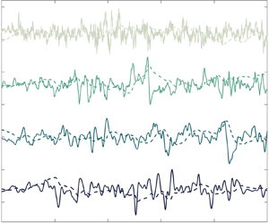
Figure 1. Numerical simulation of the set of (2.22)–(2.26) using $n=9$ layers, for $\tau _\eta =T/10$ and $\sigma ^2=1$ (see text). (a) Typical time series of the obtained processes $v_9(t)$ (dashed line) and $a_9(t)$ (solid line), as a function of time $t$. (b) Respective velocity correlation functions $\mathcal {C}_{v_9}$, estimated from numerical simulations (dots), theoretically derived from (2.28) (solid line), and the correlation function of the asymptotic process $\mathcal {C}_{v}$, of which the expression is provided in (2.29). (c) Acceleration correlation functions $\mathcal {C}_{a_n}$ using $n$ layers, $n$ ranging from 2 to 9 (from left to right), using $\sigma ^2=1$ and $\alpha _n=\alpha _9$ (2.27). Numerical estimations from time series are displayed with dots, respective theoretical expressions from (2.28) are represented with solid lines, and the asymptotic correlation function $\mathcal {C}_{a}$ (2.30) is shown with a dashed line. For the sake of clarity, all curves are normalized by their values at the origin (i.e. the respective variances). (d) Similar plot as in (c), but only the layer $n=9$ is displayed, over a shorter range of time lag $\tau$.

We display first in figure 1(a) an instance of the obtained processes $v_9(t)$ and its derivatives $a_9(t)$, over $5T$ after numerically integrating the (2.22)–(2.26). As claimed in Proposition A.2, the process $v_9$ (which correlation function is given in (2.28)) is $8$-times differentiable. Its first derivative $a_9(t)$ is consequently $7$-times differentiable; resulting in a smooth profile correlated over $\tau _\eta$. We could have performed a similar simulation using additional layers, although its estimated correlation functions of velocity and acceleration will eventually be close to the asymptotic ones of $v$ (and provided in Proposition A.2).

In figure 1(b), we present three curves corresponding to (i) the estimated correlation function $\mathcal {C}_{v_9}$ (dots), (ii) its theoretical expression (solid line), obtained when performing the integral entering in (2.28) using a symbolic calculation software, and (iii) the asymptotic correlation function $\mathcal {C}_{v}$ given in (2.29) (dashed line). The profiles collapse, making it difficult to distinguish between these three curves. The velocity correlation functions $\mathcal {C}_{v_n}$ depend weakly on $n$ (not shown). This can be understood easily since the dependence on $n$ is only really crucial at the dissipative scales; scales that are solely highlighted by a small scale quantity such as acceleration.

In this context, we present in figure 1(c) the corresponding estimated and theoretical curves $\mathcal {C}_{a_n}$ for $n$ ranging from $2$ to $9$ to observe and quantify the convergence of the acceleration correlation function towards its asymptotic regime. Recall that $\mathcal {C}_{a_2}$ corresponds to the prediction of Sawford (Reference Sawford1991) (see (2.13)), which is characteristic of the correlation function of a non-differentiable process ($\mathcal {C}_{a_2}$ is not twice differentiable at the origin). A perfect agreement between the numerical estimation based on random time series, and the theoretical expressions is observed and also derivable from (2.28). As the number of layers $n$ increases, the acceleration correlation functions become more and more curved at the origin, guaranteeing finite variance of higher-order derivatives. We superpose on this figure the associated asymptotic correlation function $\mathcal {C}_{a}$ using a dashed line. Its explicit expression is given in (2.30); $\mathcal {C}_{a_9}$ is indeed very close to $\mathcal {C}_{a}$, as shown in figure 1(d). This shows that considering $n=9$ layers is enough to reproduce the statistical behaviours of the asymptotic process, at least for velocity and acceleration, which are our main concern.

3.1. A causal multifractal random walk

Let us here review the stochastic modelling of the Lagrangian velocity proposed by Mordant et al. (Reference Mordant, Delour, Léveque, Arnéodo and Pinton2002, Reference Mordant, Delour, Lévêque, Michel, Arneodo and Pinton2003), which is based on the multifractal process of Bacry et al. (Reference Bacry, Delour and Muzy2001). This process can be considered as an OU process (2.1) forced by a non-Gaussian uncorrelated random noise, and is called the multifractal random walk (MRW). Its dynamics reads

(3.1)\begin{equation} {\rm d} u_{1,\epsilon}(t) ={-}\frac{1}{T}u_{1,\epsilon}(t)\,{\rm d} t + \sqrt{q} \exp({\gamma X_{1,\epsilon}(t)-\gamma^2\langle X_{1,\epsilon}^2\rangle})W({\rm d} t), \end{equation}

where a new random field $X_{1,\epsilon }$ is introduced. This random field is Gaussian, zero average and taken independent of the white noise instance $W({\rm d} t)$, and is thus fully characterized by its correlation function. To reproduce intermittent corrections, as they have been observed in Lagrangian turbulence (see Yeung & Pope Reference Yeung and Pope1989; Voth et al. Reference Voth, Satyanarayan and Bodenschatz1998; La Porta et al. Reference La Porta, Voth, Crawford, Alexander and Bodenschatz2001; Mordant et al. Reference Mordant, Metz, Michel and Pinton2001, Reference Mordant, Delour, Léveque, Arnéodo and Pinton2002, Reference Mordant, Delour, Lévêque, Michel, Arneodo and Pinton2003; Chevillard et al. Reference Chevillard, Roux, Lévêque, Mordant, Pinton and Arneodo2003; Biferale et al. Reference Biferale, Boffetta, Celani, Devenish, Lanotte and Toschi2004; Toschi & Bodenschatz Reference Toschi and Bodenschatz2009; Pinton & Sawford Reference Pinton, Sawford, Davidson, Kaneda and Sreenivasan2012; Bentkamp et al. Reference Bentkamp, Lalescu and Wilczek2019, and references therein), we demand the Gaussian field $X_{1,\epsilon }$ to be logarithmically correlated (Bacry et al. Reference Bacry, Delour and Muzy2001). Such a correlation structure implies in particular that the variance of $X_{1,\epsilon }$ diverges as $\epsilon \to 0$, making it difficult to give a proper mathematical meaning to such a field. This divergence is even amplified when considering its exponential, as is proposed in (3.1). Instead, we rely on an approximation procedure, at a given (small) parameter $\epsilon$, that will eventually play, loosely speaking, the role of the small time scale $\tau _\eta$ of turbulence. Such a logarithmic correlation structure has to be truncated over the large time scale $T$ in order to ensure a finite variance. These truncations are well understood from a mathematical perspective (Rhodes & Vargas Reference Rhodes and Vargas2014), and a proper limit as $\epsilon \rightarrow 0$ leads to a well-defined, canonical, random distribution.

Nonetheless, nothing is said in Bacry et al. (Reference Bacry, Delour and Muzy2001) about causality. Causal representations of multifractal random fields have been previously made by Schmitt & Marsan (Reference Schmitt and Marsan2001) and Bacry & Muzy (Reference Bacry and Muzy2003), yet these propositions are not defined as solutions of some stochastic evolutions. In order to include this important physical constraint, we define the field $X_{1,\epsilon }$ as the unique statistically stationary solution of a stochastic differential equation, that will eventually be consistent with both truncations over the time scales $\epsilon$ and $T$, and a logarithmic behaviour in between. Being Gaussian, and independent of the white noise $W({\rm d} t)$ entering in (3.1), such dynamics has to be defined as a linear operation on an independent instance of the Gaussian white noise, call it $\widetilde {W}({\rm d} t)$, such that $\langle W({\rm d} t)\widetilde {W}({\rm d} t')\rangle = 0$ at any time $t$ and $t'$. In this context, such a linear stochastic evolution has been proposed by Chevillard (Reference Chevillard2017) and Pereira, Moriconi & Chevillard (Reference Pereira, Moriconi and Chevillard2018), and reads

(3.2)\begin{equation} {\rm d} X_{1,\epsilon}(t)={-}\frac{1}{T}X_{1,\epsilon}(t)\,{\rm d} t -\frac{1}{2}\int_{-\infty}^t \left[ t-s+\epsilon\right]^{{-}3/2}\widetilde{W}({\rm d} s)\,{\rm d} t + \epsilon^{{-}1/2}\widetilde{W}({\rm d} t). \end{equation}

It can be seen as a fractional Ornstein–Uhlenbeck process of vanishing Hurst exponent (Chevillard Reference Chevillard2017; Pereira et al. Reference Pereira, Moriconi and Chevillard2018). Remark also that the underlying integration over the past with a rapidly decreasing kernel that enters in the dynamics of $X_{1,\epsilon }$ (3.2) implies that we are dealing with non-Markovian processes. A precise and comprehensive characterization of the statistical properties of the fields $X_{1,\epsilon }$ and its asymptotical log-correlated version $X_{1}\equiv \lim _{\epsilon \rightarrow 0}X_{1,\epsilon }$ can be found in Proposition A.3.

Let us focus on the statistical properties of the MRW that now includes a causal definition for the field $X_1$. We will work as much as possible, for the sake of presentation, in the asymptotic regime where we have taken the limit $\epsilon \rightarrow 0$. We keep in mind that the pointwise limit of such a process $u_1(t)=\lim _{\epsilon \to 0}u_{1,\epsilon }(t)$, where $u_{1,\epsilon }(t)$ is the unique statistically stationary solution of the SDE given in (3.1), is not straightforward to acquire, since the random field $\exp ({\gamma X_{1,\epsilon }(t)-\gamma ^2\langle X_{1,\epsilon }^2\rangle })$ becomes distributional in this limit (Rhodes & Vargas Reference Rhodes and Vargas2014). We will thus be mainly concerned with statistical quantities of the asymptotic random process $u_1$, but will perform standard calculations using the classical field $u_{1,\epsilon }(t)$ if necessary and convenient. Because we want to quantify the intermittent corrections implied by the this random distribution, we propose to compute the structure functions of the aforementioned stochastic model. Define thus the velocity increment as

(3.3)\begin{equation} \delta_\tau u_{1,\epsilon}(t) = u_{1,\epsilon}(t+\tau)-u_{1,\epsilon}(t). \end{equation}

Accordingly, define the respective asymptotic structure functions as

(3.4)\begin{equation} \mathcal{S}_{u_1,m} (\tau)=\lim_{\epsilon\rightarrow 0} \left\langle \left(u_{1,\epsilon}(t+\tau)-u_{1,\epsilon}(t)\right)^m\right\rangle. \end{equation}

In the following, we focus on the scaling properties of the structure functions of the causal MRW $u_{1}$. As a general remark, let us recall that the log-correlated field $X_1$ and the underlying white noise $W$ entering in the dynamics of $u_{1,\epsilon }$ are taken independently. This implies that all odd-order structure functions vanish, namely $\mathcal {S}_{u_1,2m+1}=0$ with $m\in \mathbb {N}$. Regarding the second-order structure function, it is the same as the one obtained from the OU process $v_1$ (2.1), and given by

(3.5)\begin{equation} \mathcal{S}_{u_1,2} (\tau)=\mathcal{S}_{v_1,2} (\tau) = qT\left[1-{\rm e}^{-\frac{|\tau|}{T}}\right]\mathop{\sim}\limits_{\tau\rightarrow 0^+} q\tau. \end{equation}

On the contrary, the fourth-order structure function is impacted by intermittency, and we get, under the condition $4\gamma ^2<1$,

(3.6)\begin{equation} \mathcal{S}_{u_1,4} (\tau)\mathop{\sim}\limits_{\tau\rightarrow 0} \frac{3}{1-6\gamma^2+8\gamma^4}q^2\tau^2\left(\frac{\tau}{T}\right)^{{-}4\gamma^2}{\rm e}^{4\gamma^2c(0)}, \end{equation}

where the constant $c(0)$ is given in (A 18). More generally, it is then possible to obtain an estimation of the $(2m)$th-order structure functions that reads, for $2m(m-1)\gamma ^2<1$,

(3.7)\begin{equation} \mathcal{S}_{u_1,2m} (\tau)\mathop{\propto}\limits_{\tau\rightarrow 0} q^{m}\tau^m\left(\frac{\tau}{T}\right)^{{-}2m(m-1)\gamma^2}, \end{equation}

indicating that the causal MRW exhibits a log-normal spectrum. We gather all the proofs of these propositions in appendix B.

3.2. An infinitely differentiable causal multifractal random walk

Our proposition is herein made of a causal stochastic process representative of the statistical behaviour of Lagrangian velocity in homogeneous and isotropic turbulent flows at a given finite Reynolds number (equivalently for a finite ratio $\tau _\eta /T$). We are demanding a statistically stationary process, correlated over a large time scale $T$, that is infinitely differentiable (giving meaning to the respective acceleration process), acquiring rough and intermittent behaviours as the small time scale $\tau _\eta$ goes to zero, i.e. in the infinite Reynolds number limit.

Assume $n \ge 2$ and consider the following system of embedded differential equations

(3.8)\begin{gather} \frac{{\rm d} u_{n,\epsilon}}{{\rm d} t} ={-}\frac{1}{T}u_{n,\epsilon}(t)+ \exp\left({\gamma X_{n,\epsilon}(t)-\frac{\gamma^2}{2}\langle X_{n,\epsilon}^2\rangle}\right) f_{n-1}(t), \end{gather}

(3.9)\begin{gather}\frac{{\rm d} f_{n-1}}{{\rm d} t} ={-}\frac{\sqrt{n-1}}{\tau_{\eta}}f_{n-1}(t)+ f_{n-2}(t), \end{gather}

(3.10)\begin{gather}\cdots \end{gather}

(3.11)\begin{gather}\frac{{\rm d} f_{2}}{{\rm d} t} ={-}\frac{\sqrt{n-1}}{\tau_{\eta}}f_{2}(t)+ f_{1}(t), \end{gather}

(3.12)\begin{gather}{\rm d} f_1 ={-}\frac{\sqrt{n-1}}{\tau_\eta}f_1(t) \,{\rm d} t + \sqrt{\beta_{n}}W({\rm d} t), \end{gather}

with

(3.13)\begin{equation} \beta_n=\left( \frac{n-1}{\tau_\eta^2}\right)^{n-1}\frac{\sigma^2\sqrt{4{\rm \pi}\tau_\eta^2}}{T\displaystyle\int_{0}^\infty {\rm e}^{-\frac{h}{T}}{\rm e}^{{-}h^2/(4\tau_\eta^2)}{\rm e}^{\gamma^2\mathcal{C}_{X}(h)}\, {\rm d} h}. \end{equation}

In the system above, the causal process $X_{n,\epsilon }$ obeys the set of stochastic differential equations

(3.14)\begin{gather} \frac{{\rm d} X_{n,\epsilon}}{{\rm d} t} ={-}\frac{1}{T}X_{n,\epsilon}(t)+ \sqrt{\tilde{\beta}_n}\,\tilde{f}_{n-1,\epsilon}(t), \end{gather}

(3.15)\begin{gather}\frac{{\rm d} \tilde{f}_{n-1,\epsilon}}{{\rm d} t} ={-}\frac{\sqrt{n-1}}{\tau_{\eta}}\tilde{f}_{n-1,\epsilon}(t)+ \tilde{f}_{n-2,\epsilon}(t), \end{gather}

(3.16)\begin{gather}\cdots \end{gather}

(3.17)\begin{gather}\frac{{\rm d} \tilde{f}_{2,\epsilon}}{{\rm d} t} ={-}\frac{\sqrt{n-1}}{\tau_{\eta}}\tilde{f}_{2,\epsilon}(t)+ \tilde{f}_{1,\epsilon}(t), \end{gather}

(3.18)\begin{gather}{\rm d} \tilde{f}_{1,\epsilon} ={-}\frac{\sqrt{n-1}}{\tau_\eta}\tilde{f}_{1,\epsilon}(t) \,{\rm d} t -\frac{1}{2}\int_{-\infty}^t \left[ t-s+\epsilon\right]^{{-}3/2}\widetilde{W}({\rm d} s)\,{\rm d} t + \epsilon^{{-}1/2}\widetilde{W}({\rm d} t), \end{gather}

with

(3.19)\begin{equation} \tilde{\beta}_n=\left( \frac{n-1}{\tau_\eta^2}\right)^{n-1}. \end{equation}

where $W$ and $\widetilde {W}$ are two independent copies of the Wiener process.

Similar to the Gaussian infinitely differentiable process $v$ established in the first part, we show in the following Proposition A.5 that the process $u$, obtained once the procedure depicted in the set of embedded differential equations ((3.8)–(3.12)) is iterated an infinite number of times $n\rightarrow \infty$, and when the small parameter $\epsilon$ goes to zero, converges to a well-defined limit. Once again, the choice made for the white noise weight $\beta _n$ (3.13) ensures that the variance of the limiting process $u$ is finite with $\langle u^2\rangle =\sigma ^2$. Its precise value will become evident when we compute the correlation function $\mathcal {C}_f(\tau )=\langle \,f(t)f(t+\tau )\rangle$ of the force $f$ when $n\to \infty$ (see (A 29)).

Similarly, the precise choice for the coefficient $\tilde {\beta }_n$ (3.19) entering in the dynamics of $X_{n,\epsilon }$ (3.14) is dictated by the necessity that, in an asymptotic way, when both $\epsilon \to 0$ and $\tau _\eta \rightarrow 0$, and for any number of layers $n$, $X_{n}$ becomes logarithmically correlated in an appropriate manner. As far as the process $X_{n,\epsilon }$ is concerned, these limits can be taken in an arbitrary way since they commute. The small parameters $\epsilon$ and $\tau _\eta$ have a similar physical interpretation, they mimic finite Reynolds number effects. We define them a priori as separate entities and seek for limits independently for the sake of generality. More precisely, $\epsilon$ is taken to be finite to make sense of the dynamics of $\tilde {f}_{1,\epsilon }$ as it is proposed in (3.18). Remark finally that the multiplicative chaos entering into the dynamics of $u_{n,\epsilon }$ (3.8) is renormalized by a smaller constant $\exp (({\gamma ^2}/{2})\langle X_{n,\epsilon }^2\rangle )$ than in its non-differentiable version $u_{1,\epsilon }$ (3.1), where there typically exists a larger normalization constant $\exp (\gamma ^2\langle X_{n,\epsilon }^2\rangle )$. It is related to the finite correlation of the of the term $f_{n-1}$ entering in (3.8), contrary to the dynamics proposed in (3.1), where a white noise $W({\rm d} t)$ enters.

As a general remark, notice that the dynamics depicted by the set of embedded differential equations ((3.8)–(3.12)) coincides with the dynamics of the Gaussian process $v_n$ ((2.22)–(2.26)) when we consider the particular value $\gamma =0$. In other words, the non-intermittent limit of the process $u_{n,\epsilon }$ is Gaussian, and coincides with the process $v_n$ of § 2.3.

Before establishing the statistical behaviour of the asymptotic process $u$, let us first focus on the statistical properties of $X_{n,\epsilon }$ that we gather and derive in Proposition A.4. Keeping in mind that whatever the ordering of the limits $n\rightarrow \infty$ and $\epsilon \rightarrow 0$, the correlation function of $X_{n,\epsilon }$ converges towards a well-defined function $\mathcal {C}_{X}(\tau )$ (A 21), the value of which at the origin diverges logarithmically with $\tau _\eta$ as $\tau _\eta \to 0$ (A 24). Actually, in this limit of infinite Reynolds numbers, $\mathcal {C}_{X}(\tau )$ converges towards $\mathcal {C}_{X_1}(\tau )$ (A 25), as expected.

We now proceed with the covariance structure of the limiting process $u$. We summarize and demonstrate in Proposition A.5 the main second-order statistical properties of velocity $u$ and acceleration $a$. We first derive the exact velocity correlation function $\mathcal {C}_u(\tau )$ in the joint commuting limit $\epsilon \to 0$ and $n\to \infty$ (A 28). This shows that, whereas $\mathcal {C}_u(\tau )$ depends weakly on intermittent corrections in the dissipative range, it loses this property as $\tau _\eta /T\to 0$ and coincides with the correlation function of the OU process $\mathcal {C}_{v_1}(\tau )$ (A 30). Similarly, the acceleration correlation function $\mathcal {C}_a(\tau )$ can be derived (A 32). From there, we show that acceleration variance diverges as $T/\tau _\eta$ as the Reynolds number increases (A 34).

Let us remark that the proposed stochastic model of velocity, $u$, that we claim to be intermittent in a precise way and defined in Proposition A.6, predicts that, as far as the covariance of $u$ is concerned, it is similar to an Ornstein–Uhlenbeck process at infinite Reynolds number, independently of any intermittency corrections. This is consistent with the standard phenomenology of Lagrangian turbulence. The predicted acceleration variance (A 34) does not exhibit either intermittent corrections: this precise behaviour of acceleration variance with respect to the Reynolds number is at odds with the extrapolations that can be made from numerical simulations (cf. Ishihara et al. (Reference Ishihara, Kaneda, Yokokawa, Itakura and Uno2007) and the discussion that we propose in § 5.3). We will see and develop in § 5 that the multifractal formalism allows the understanding of how the velocity correlation does not get impacted by intermittency at infinite Reynolds numbers, whereas the acceleration variance does.

Let us now present the intermittent, i.e. multifractal, properties of the velocity process $u$, as they can be seen on higher-order structure functions (see Proposition A.6). As shown previously, the correlations of $u$ and the OU process $v_1$ coincide as $\tau _\eta \to 0$. The same goes for the second-order structure function (A 37). Whereas showing that the fourth-order structure function of $u$ coincides with that of the causal MRW process $u_1$ as first $\epsilon \to 0$ and then $\tau _\eta \to 0$ is obvious (A 38), the reversed order of limits is more involved. We nonetheless propose an approximation procedure that confirms that $u$ and $u_1$ possess the same intermittent properties (A 39). All statements and proofs can be found in Proposition A.6 and appendix C.

3.3. A second numerical illustration

3.3.1. An efficient algorithm under the periodic approximation

In this section we propose a numerical algorithm able to reproduce in a realistic and efficient fashion the statistical behaviour of the process $u$, which statistical properties are detailed in Propositions A.5 and A.6. As we have seen, the process $u$, contrary to the Gaussian process $v$ of § 2.3, obeys a non-Markovian dynamics. More precisely, for the process $X(t)$ at a given time $t$, the limiting solution, as the number of layers $n$ goes to infinity and the small parameter $\epsilon$ goes to 0, of the system of embedded stochastic differential equations (3.14)–(3.18), requires the knowledge of its entire past. It is thus tempting to use the discrete Fourier transform to solve its dynamics. We will incidentally generate periodic solutions of this non-Markovian dynamics. Since we will consider in the sequel very long trajectories, of order $10^5$ times the largest time scale $T$ of the process, all aliasing effects will be negligible. This periodic approximation is well justified. As argued in § 2.4, simulations of the limiting process with $n\to \infty$ require the causal factorization of covariance functions of underlying Gaussian components, a procedure which is not simple. Furthermore, the limit $\epsilon \to 0$ is also complicated to obtain from a numerical point of view, and therefore, we will perform simulations for a finite $n$ number of layers, and for a finite $\epsilon >0$.

Consider first an estimator for the discrete process $\widehat {X}_{n,\epsilon }[t]$ of the continuous solution $X_{n,\epsilon }(t)$ of the coupled system (3.14)–(3.18). Let us introduce the convolution product $\ast$, which is defined as, for any two functions $g_1$ and $g_2$,

\[ \left(g_1\ast g_2\right)(\tau) = \int_{\mathbb{R}}g_1(t)g_2(\tau-t)\,{\rm d} t, \]

with the corresponding shorthand notation,

\[ g^{{\ast} n}=\underbrace{g \ast g \ast \cdots \ast g}_{n}. \]

In the statistically stationary regime, the continuous expression of the Gaussian process $X_{n,\epsilon }(t)$ reads

(3.20)\begin{equation} X_{n,\epsilon}(t)=\sqrt{\widetilde{\beta}_n} \left(g_T\ast g_{\frac{\tau_\eta}{\sqrt{n-1}}}^{{\ast} (n-1)}\ast \left( h_\epsilon+\epsilon^{{-}1/2}\delta\right) \ast \widetilde{W} \right)(t), \end{equation}

where the multiplicative factor $\widetilde {\beta }_n$ is given in (3.19), and recall that $g_\tau (t) = {\rm e}^{-t/\tau }1_{t\ge 0}$. We also include $h_\epsilon (t) = -\frac {1}{2}(t+\epsilon )^{-3/2}1_{t\ge 0}$ and $\delta (t)$ stands for the Dirac delta function.

Now in the discrete setting, call $N$ the number of collocation points, $T_{{{\textit{tot}}}}$ the total length of the simulation and ${\rm \Delta} t$ the time step. As already mentioned, make sure that $T_{{{\textit{tot}}}}=N{\rm \Delta} t \gg T$ to prevent aliasing errors. In the aforementioned periodic framework, the discrete estimator $\widehat {X}_{n,\epsilon }[t]$ of the continuous solution $X_{n,\epsilon }(t)$ (3.20) reads

(3.21)\begin{align} \widehat{X}_{n,\epsilon}[t]=\sqrt{\widetilde{\beta}_n} \mbox{DFT}^{{-}1}\left( \mbox{DFT}\left(g_T \right)\mbox{DFT}^{n-1}\left(g_{\frac{\tau_\eta}{\sqrt{n-1}}} \right) \mbox{DFT}_c\left(h_\epsilon \right) \mbox{DFT}\left(\widetilde{W} \right) \right)[t]\times ({\rm \Delta} t)^{n}, \end{align}

where we have introduced the discrete Fourier transform (DFT). It also enters in the expression given in (3.21), properly discretizing and periodizing forms of the continuous functions $g_\tau (t)$ at various time scales $\tau$ and $h_\epsilon (t)$. Notice that in the continuous framework, $\int _\mathbb {R} h_\epsilon (t)\,{\rm d} t=-\epsilon ^{-1/2}$ is the value at the origin of frequencies of the Fourier transform (FT) of $h_\epsilon$, such that $\mbox {FT}(h_\epsilon +\epsilon ^{-1/2}\delta )(\omega )=\mbox {FT}(h_\epsilon )(\omega )-\mbox {FT}(h_\epsilon )(0)$. This justifies the shorthand notation $\mbox {DFT}_c(h_\epsilon )[\omega ] = \mbox {DFT}(h_\epsilon )[\omega ] -\mbox {DFT}(h_\epsilon )[0]$ in (3.21). Finally, we have noted $\widetilde {W}[t]$ an instance of the white noise field, comprised of $N$ independent Gaussian random variables of zero average and variance ${\rm \Delta} t$. The $({\rm \Delta} t)^{n}$ factor originates from the convolution by the kernel $g_T(t)$ and $(n-1)$ convolutions by the kernel $g_{{\tau _\eta }/{\sqrt {n-1}}}$.

In a similar manner, the numerical, discretized and periodized estimator $\hat {u}_{n,\epsilon }$ of the continuous solution $u_{n,\epsilon }$ of the coupled system (3.8)–(3.12) in the statistically stationary regime, which reads

(3.22)\begin{equation} u_{n,\epsilon}(t)=\sqrt{\beta_n} \left(g_T\ast g_{\frac{\tau_\eta}{\sqrt{n-1}}}^{{\ast} (n-1)}\ast \left( \frac{{\rm e}^{\gamma \widehat{X}_{n,\epsilon}}}{ \exp\left({\dfrac{\gamma^2}{2}\langle \widehat{X}_{n,\epsilon}^2 \rangle}\right)} W\right) \right)(t), \end{equation}

can be written as

(3.23)\begin{align} \hat {u}_{n,\epsilon}[t] & =\sqrt{\beta_n} \mbox{DFT}^{{-}1}\left( \mbox{DFT}\left(g_T \right)\mbox{DFT}^{n-1}\left(g_{\frac{\tau_\eta}{\sqrt{n-1}}} \right) \mbox{DFT}\left(\frac{{\rm e}^{\gamma \widehat{X}_{n,\epsilon}}}{\exp\left({\dfrac{\gamma^2}{2}\langle \widehat{X}_{n,\epsilon}^2 \rangle}\right)} W \right) \right)[t] \notag \\ & \quad \times ({\rm \Delta} t)^{n-1}, \end{align}

where $\beta _n$ is provided in (3.13), and recall that the white noise $W$ is independent of $\widetilde {W}$ that enters in (3.21). The fact that we multiply by $({\rm \Delta} t)^{n-1}$ the overall expression 3.23, instead of $({\rm \Delta} t)^{n}$ (as in (3.21)), originates from the white (i.e. distributional) nature of $W$, whereas $\widetilde {W}$ is already smoothed out by the kernel $h_\epsilon$.

The time step ${\rm \Delta} t$ has to be chosen to be smaller than the smallest scale of motion, that is ${\tau _\eta }/{\sqrt {n-1}}$. Furthermore, we are interested in performing a realistic simulation of the limiting process $u$, obtained in the limit $\epsilon \to 0$, at a given finite $\tau _\eta$. A convenient choice for $\epsilon$ is to take it proportional to ${\rm \Delta} t$, such that both of them go to zero in the continuous limit. In subsequent simulations, we find it appropriate to choose

(3.24a,b)\begin{equation} {\rm \Delta} t=\frac{\tau_\eta}{200\sqrt{n-1}} \quad\mbox{and}\quad \epsilon = 5{\rm \Delta} t. \end{equation}

This choice gives numerical stability and a proper illustration of the exact statistical quantities provided in Propositions A.5 and A.6 for the range of investigated values of $\tau _\eta$ (see the following § 3.3.2). To prevent aliasing errors, we work with a large number of collocation points $N=2^{32}$, such that $T_{{{\textit{tot}}}}=N{\rm \Delta} t$ is always much larger than $T$.

3.3.2. Numerical results and comparisons with theoretical predictions

Without loss of generality, we take $T=1$. We numerically perform the (discrete) Fourier transforms as they are detailed in (3.21) and (3.23), using six values for $T/\tau _\eta$, that is 10, 20, 50, 100, 200 and 500. Keeping in mind that $\tau _\eta$ is a fairly good representation of the Kolmogorov time scale, these values correspond to an extended range of Reynolds numbers. Choosing for ${\rm \Delta} t$ and $\epsilon$ the values depicted in (3.24a,b), working with $N=2^{32}$ collocation points and $n=9$ layers, we find in the worst scenario corresponding to the smallest $\tau _\eta$ a total time of simulation $T_{{{\textit{tot}}}}=N{\rm \Delta} t \approx 10^4T$, preventing any aliasing effects. As will be precisely quantified when we discuss intermittent corrections, we find the particular value

(3.25)\begin{equation} \gamma^2=0.085, \end{equation}

representative of the level of intermittency seen in numerical simulations of the Navier–Stokes equations, consistent with previous estimations (see Mordant et al. Reference Mordant, Delour, Léveque, Arnéodo and Pinton2002; Chevillard et al. Reference Chevillard, Roux, Lévêque, Mordant, Pinton and Arneodo2003; Biferale et al. Reference Biferale, Boffetta, Celani, Devenish, Lanotte and Toschi2004; Chevillard et al. Reference Chevillard, Castaing, Arneodo, Lévêque, Pinton and Roux2012 and references therein). Forthcoming statistical quantities are averaged over three independent instances of these trajectories.

For the sake of clarity, we omit the hat on the simulated discrete version of $u_{9,\epsilon }$, and display in figure 2(a,b) two instances of this stochastic process for the largest $\tau _\eta =T/10$ (lowest Reynolds number) and the smallest $\tau _\eta =T/500$ (highest Reynolds number) ratios of the small over the large time scales. Velocity is represented using a dot-dashed line, whereas the respective acceleration with a solid line. All time series are divided by their respective standard deviation for the sake of comparison. In the low Reynolds number case (figure 2a), we observe that indeed velocity is correlated over $t$, whereas acceleration is correlated over a shorter time scale $\tau _\eta$. In the highest Reynolds number case (figure 2b), we can definitely observe the scale decoupling between the large $T$ and the small $\tau _\eta$ time scales. Also, notice that the statistics of acceleration are evidently non-Gaussian. This is a manifestation of the intermittency phenomenon, which is modelled by the multiplicative chaos that enters into the construction. These non-Gaussian fluctuations would be enhanced by a higher value of $\gamma$ (data not shown) than the one chosen presently (3.25). We will come back to this point while discussing figure 3.

Figure 2. Numerical simulation, in a periodical fashion, of the set of (3.8)–(3.12) using $n=9$ layers, for 6 values of $\tau _\eta$, that is $T/\tau _\eta =$ 10, 20, 50, 100, 200, 500 and $\sigma ^2=1$. See the description of the algorithm in § 3.3.1, and the choice made for other parameters in § 3.3.2. (a) Typical time series of the obtained processes $u_9(t)$ (dashed line) and $a_9(t)$ (solid line), as a function of time $t$, for $T/\tau _\eta =10$. For the sake of comparison, all time series are normalized by their standard deviation. (b) Similar time series as in (a), but for $T/\tau _\eta =500$. (c) Respective velocity correlation functions $\mathcal {C}_{u_9}$ for the six different values of $\tau _\eta$, estimated from numerical simulations (dots), compared with their asymptotic theoretical prediction $\mathcal {C}_{u}$ (A 28) (solid line). (d) Respective acceleration correlation functions $\mathcal {C}_{a_9}$ compared with the asymptotic correlation function $\mathcal {C}_{a}$ (A 32). For the sake of clarity, all curves are normalized by their values at the origin (i.e. the respective variances).

Figure 3. Illustration of the behaviour of higher-order statistics of the processes studied in figure 2. (a) Logarithmic representation of the second-order structure function, estimated from the times series of the six different values of $\tau _\eta$ (solid lines), and compared with their asymptotic prediction provided in (A 37) (dashed line). (c) Similar logarithmic process as in (a), but for the flatness of velocity increments. We superimpose the theoretical prediction based on (3.6) (see the devoted discussion in § 3.3.2). (b) Estimation of the probability density functions of velocity increments for scales logarithmically spanning the accessible range of scales displayed in (a,c), and for $\tau _\eta /T=1/10$. (d) Similar plot as in (b) but for $\tau _\eta /T=1/500$.

We present in figure 2 the velocity (c) and acceleration (d) correlation functions. Results from the numerical simulation of (3.21) and (3.23) for the six values of $\tau _\eta$ are displayed using dots; we superimpose the theoretical expressions provided in (A 28) and (A 32). Concerning the velocity correlations (figure 2c), we can notice the striking agreement between the numerical estimation based on time series of $u_{9,\epsilon }$ and the limiting theoretical expression (A 28), as was already observed in the Gaussian case (figure 1). Furthermore, as expected, the dependence on $\tau _\eta$ is very weak. This can be easily understood by realizing that the velocity is a large scale quantity, mostly governed by the physics taking place at $T$. In this regard, acceleration correlation functions will highlight the physics ruling phenomena which occur at $\tau _\eta$ and are displayed in figure 2(d). All curves are normalized by the respective value at the origin (i.e. the acceleration variance). The low Reynolds number case (largest $\tau _\eta$) is easily recognizable; this is the curve going the most negative after the zero crossing. As $\tau _\eta$ decreases, $\mathcal {C}_a(\tau )$ is closer to 0. This is consistent with the constraint that the integral of this curve has to vanish, as a consequence of statistical stationarity. Once again, the collapse of the numerically estimated $\mathcal {C}_{a_9}(\tau )$ (dots) onto the limiting theoretical expression given in (A 32) (solid line) is excellent.

Let us now focus on the precise quantification on the intermittency phenomenon. We display in figure 3(a,c) the behaviour across scales $\tau$ of the structure functions $\mathcal {S}_{u_{n,\epsilon },m}=\langle (\delta _\tau u_{n,\epsilon })^m \rangle$ of the simulated process $u_{n,\epsilon }$. We then compare them with our theoretical predictions (Proposition A.6) obtained in the asymptotic regime $n\to \infty$, $\epsilon \to 0$, $\tau _\eta \to 0$ and finally $\tau \to 0$ (limits are taken in this order).

We present in figure 3(a) the scaling behaviour of the second-order structure function $\mathcal {S}_{u_{9,\epsilon },2}(\tau )=\langle (\delta _\tau u_{9,\epsilon })^2 \rangle$ (solid lines) for the 6 values of $\tau _\eta$ that we formerly detailed. Notice that, in this representation, $\mathcal {S}_{u_{9,\epsilon },2}(\tau )$ is normalized by $2\langle u^2_{9,\epsilon }\rangle$, such that it goes to unity at large arguments $\tau \gg T$. We recover at small scales $\tau \ll \tau _\eta$ the dissipative behaviour $\mathcal {S}_{u_{9,\epsilon },2}(\tau )\propto \tau ^2$, which is a consequence of the differentiable nature of the process. In the inertial range $\tau _\eta \ll \tau \ll T$, as expected by our theoretical prediction (A 37), we get a behaviour similar to an OU process, that is $\mathcal {S}_{u_{9,\epsilon },2}(\tau )\propto \tau$. We superimpose using a dashed line the expected behaviour from an OU process, namely $S_{u_{1},2}(\tau )=2\langle u^2_{1}\rangle (1-{\rm e}^{-|\tau |/T})$. We indeed observe that it describes with great accuracy the scaling behaviour of $\mathcal {S}_{u_{9,\epsilon },2}(\tau )$ in the inertial range and at larger scales. The second-order statistics of $u_{9,\epsilon }$ are well described by our asymptotic predictions in this range of scales. Similar conclusions were obtained while describing velocity correlation function in figure 2(c).

As mentioned in Proposition A.6, only fourth-order statistics and higher are impacted by intermittency. To check this, we represent in figure 3(c) the scaling behaviour of the flatness of velocity increments, that is $\mathcal {S}_{u_{9,\epsilon },4}/\mathcal {S}_{u_{9,\epsilon },2}^2$ (solid lines), for the 6 different values of $\tau _\eta$, in a logarithmic fashion. As shown, flatnesses are normalized by 3, i.e. the value obtained for Gaussian processes. As we can observe, flatnesses are close to 3 at large scales $\tau \ge T$, and then increase in the inertial range as a power law, before saturating in the dissipative range $\tau \le \tau _\eta$. This saturation is typical of differentiable processes: a Taylor series of increments makes the dependence on $\tau$ disappear. We superimpose on this plot, using a dashed line, the theoretical prediction that we made for MRW (3.6) without the unjustified additional free parameter. We indeed see that the power-law exponent is given by $-4\gamma ^2$, and that the multiplicative constant is close to the one derived for the non-differentiable MRW (3.6). This theoretical prediction seems to be more and more representative of the intermittent properties of $u_{9,\epsilon }$ as $\tau _\eta$ gets smaller and smaller. This indicates that the constant $c_{\gamma ,4}$ which is tedious to compute in an exact fashion (but easily accessible in the approximate framework developed in appendix C) for the infinitely differentiable MRW (A 39) is the same as in the non-differentiable case (3.6). This shows that the limits $\epsilon \to 0$ and $\tau _\eta \to 0$ commute at the fourth order too ((A 38) and (A 39)). This remains to be done on rigorous grounds.

Finally, to illustrate the intermittent behaviour of the process $u_{9,\epsilon }$, we display in figure 3(b,d) the probability density functions (PDFs) of velocity increments at various scales, from large to small: (b) $\tau _\eta /T=1/10$ and (d) $\tau _\eta /T=1/500$. We indeed observe the continuous shape deformation of these PDFs as the scale $\tau$ decreases in length, being Gaussian at large scales $\tau \ge T$, and strongly non-Gaussian in the dissipative range. In a manner consistent with the behaviour of the flatnesses (figure 3c), the acceleration PDF, obtained when $\tau \ll \tau _\eta$, is less and less Gaussian as $\tau _\eta$ diminishes in size.

4.1. Description of the datasets

We consider in this article two sets of data that have been made freely accessible to the public. We focus our attention on statistically homogeneous and isotropic numerical flows obtained by solving the Navier–Stokes equations in a periodic box. Lagrangian trajectories are then extracted from the time evolution of the Eulerian fields while integrating the positions of tracer particles, initially distributed homogeneously in space. The first set concerns a direct numerical simulation (DNS) at a moderate Taylor based Reynolds number $\mathcal {R}_\lambda =185$, referenced in Bec et al. (Reference Bec, Biferale, Boffetta, Celani, Cencini, Lanotte, Musacchio and Toschi2006), Bec et al. (Reference Bec, Biferale, Cencini, Lanotte and Toschi2011), which can be downloaded from https://turbase.cineca.it/. The second dataset concerns a higher Taylor based Reynolds number $\mathcal {R}_\lambda =418$, hosted at Johns Hopkins Turbulence Database (JHTDB) (see http://turbulence.pha.jhu.edu). Details on this DNS and how to extract the Lagrangian trajectories can be found in Li et al. (Reference Li, Perlman, Wan, Yang, Burns, Meneveau, Burns, Chen, Szalay and Eyink2008) and Yu et al. (Reference Yu, Kanov, Perlman, Graham, Frederix, Burns, Szalay, Eyink and Meneveau2012). Relevant parameters and specificities of these datasets and of the Lagrangian trajectories are given in table 1.

Table 1. Summary of relevant physical parameters of the two sets of DNS data. Resolution of the Eulerian fields, Taylor based Reynolds number $\mathcal {R}_\lambda$ and Kolmogorov dissipative time scale $\tau _K$ (4.2) are provided in relevant publications (see text). The Lagrangian integral time scale $T_L$ is defined in (4.1) and is computed from our statistical estimation of the velocity correlation function.

4.2. Definition and estimation of the Lagrangian integral time scale

Let us now make a connection between the present modelling approach, and its parameters, and numerical investigations. To do so, we have to consider quantities that can be extracted from DNS data, and show how to relate them to the free parameters entering in the definition of the stochastic process $u$, which are at a given Reynolds number $\tau _\eta$, $T$ and $\gamma$.

Call $T_L$ the Lagrangian integral time scale, defined as the integral of the velocity correlation function, i.e.

(4.1)\begin{equation} T_L = \int_{0}^\infty \frac{\mathcal{C}_u(\tau)}{\mathcal{C}_u(0)}\, {\rm d} \tau, \end{equation}

where $u$ stands for any Lagrangian velocity components extracted from DNS data, or the present stochastic model.

On the one hand, the definition of $T_L$ (4.1) is appealing because it can be applied to and estimated from velocity time series coming indifferently from DNS or the model. On the other hand, it requires proper statistical convergence of the velocity correlation $\mathcal {C}_u(\tau )$ that is especially difficult to get from DNS at large time scales $\tau$ close to the velocity decorrelation time scale. This is even more true when considering experimental data (see a recent discussion on this by Huck, Machicoane & Volk (Reference Huck, Machicoane and Volk2019)) in which the duration of trajectories are usually shorter. Moreover, on the entire accessible statistical sample, made of tens (even one hundred in the moderate Reynolds number case) of thousands of trajectories for each of the three velocity components, we have observed a non-negligible level of anisotropy for both sets of data, the standard deviation of the variance of the three velocity components is of the order of $20\,\%$ of the average variance. We found this level of anisotropy surprising given the isotropic and periodic boundary conditions of the advecting flow. We are forced to reach the conclusion that, in both cases, trajectories are not long enough to guarantee statistical isotropy. This has consequences for the estimation of $T_L$. Nonetheless, and because we expect ultimately that the flow, and incidentally its Lagrangian trajectories, are isotropic, we average the velocity correlation function over the three components, keeping in mind that the lack of statistical convergence can imply a non-negligible error in the estimation of this large time scale. We gather our findings in table 1. Notice that this observed anisotropy on the velocity variance has weak impact on the acceleration correlation function once normalized by its value at the origin (data not shown). This can be understood by realizing that acceleration is governed by the small scales of the flow, and velocity by the large ones.

4.3. Statistical analysis of the DNS datasets

We display in figure 4(a,c) the numerical estimation of velocity and acceleration correlation functions based on the Lagrangian trajectories extracted from DNS, at moderate Reynolds number $\mathcal {R}_\lambda =185$ (using open circles ) and at high Reynolds number $\mathcal {R}_\lambda =418$ (using open squares ). As $\mathcal {C}_u(\tau )$ is concerned (figure 4a), we normalize time lags $\tau$ by a large time scale $T$ coming from the adopted calibration procedure of our model, and that we properly define in § 4.4.2. At this level of discussion, keep in mind that $T$ is very close to $T_L$ (4.1). Concerning $\mathcal {C}_a(\tau )$ (figure 4c), we normalize time lags $\tau$ by the Kolmogorov time scale $\tau _K$ that reads

(4.2)\begin{equation} \tau_K = \sqrt{\frac{\nu}{\langle \varepsilon \rangle}}, \end{equation}

where $\nu$ is the kinematic viscosity and $\langle \varepsilon \rangle$ the average viscous dissipation per unit of mass. Interestingly, we observe that, in this representation, where scales are normalized by $\tau _K$, $\mathcal {C}_a(\tau )$ crosses zero at a Reynolds number independent time scale. Call such a scale $\tau _0$, thus defined by $\mathcal {C}_a(\tau _0)=0$. Indeed, this was already observed in numerical and laboratory flows (Yeung et al. Reference Yeung, Pope, Kurth and Lamorgese2007; Huck et al. Reference Huck, Machicoane and Volk2019): the zero-crossing time scale of acceleration has a universal (i.e. Reynolds number independent) behaviour with respect to the Kolmogorov time scale $\tau _K$ (4.2), such that

(4.3)\begin{equation} \tau_0 \approx 2.2\,\tau_K, \end{equation}

in the range of investigated Kolmogorov time scales. In our case and to be more precise, we find $\tau _0 = 2.11\,\tau _K$ at $\mathcal {R}_\lambda =185$, and $\tau _0 = 2.14\,\tau _K$ at $\mathcal {R}_\lambda =418$, indeed very close to previous findings of Yeung et al. (Reference Yeung, Pope, Kurth and Lamorgese2007) (4.3). In the sequel, we will use this fact to fully calibrate our model, in particular while relating its free parameter $\tau _\eta$ to the characteristics of the numerical flows. We will revisit this point in § 4.4.2.

Figure 4. Comparison of DNS data with model predictions. (a) Estimation of the velocity correlation function from DNS data (using for $\mathcal {R}_\lambda = 185$ and for $\mathcal {R}_\lambda = 418$. We superimpose theoretical predictions using (A 28), for the set of values of the parameters $\tau _\eta$ and $T$ given by our calibration procedure presented in § 4.4.2, and for a prescribed value for $\gamma$ (3.25). Time lags are normalized by the calibrated time scale $T$. (b) Same plot as in (a) but for the second-order structure function. (c) Similar plot as in (a,b) but for the acceleration correlation function, normalized by its value at the origin. Superimposed theoretical predictions are based on the exact expression (A 32). (d) Similar plot as in (a,b) but for the flatnesses of velocity increments. Theoretical prediction are obtained thanks to a numerical estimation of velocity time series of the model, in the spirit of § 3.3.2, with the values of the free parameters obtained from our calibration procedure presented in § 4.4.2 and for a prescribed value for $\gamma$ (3.25).

Similarly, we display the scaling behaviour of the second-order structure function $\mathcal {S}_{u,2}$ (figure 4b) and of the flatness of the velocity increments (figure 4d). We can easily observe the three expected ranges of scales: the dissipative one with $\mathcal {S}_{u,2}(\tau )\propto \tau ^2$, the inertial one with $\mathcal {S}_{u,2}(\tau )\propto \tau$ and the saturation towards $2\langle u^2\rangle$ at larger scales. Concerning the flatness, similar behaviour is observed, saturation at the Gaussian value 3 at large scales, and a power-law behaviour in the inertial range, reminiscent of the intermittency phenomenon. We furthermore observe a more rapid increase in the intermediate dissipative range, and then a Reynolds number dependent saturation towards the flatness of acceleration. This is a known effect of the fine structure of turbulence, linked to subtle differential action of the viscosity that depends on the local regularity of the velocity field (Chevillard et al. Reference Chevillard, Roux, Lévêque, Mordant, Pinton and Arneodo2003; Chevillard, Castaing & Lévêque Reference Chevillard, Castaing and Lévêque2005; Chevillard et al. Reference Chevillard, Castaing, Lévêque and Arneodo2006; Arneodo et al. Reference Arneodo, Benzi, Berg, Biferale, Bodenschatz, Busse, Calzavarini, Castaing, Cencini and Chevillard2008; Benzi et al. Reference Benzi, Biferale, Fisher, Lamb and Toschi2010; Chevillard et al. Reference Chevillard, Castaing, Arneodo, Lévêque, Pinton and Roux2012). This phenomenon is well reproduced by the phenomenology of the intermittency phenomenon developed in the framework of the multifractal formalism (Paladin & Vulpiani Reference Paladin and Vulpiani1987; Frisch Reference Frisch1995). We will develop these ideas in § 5.

4.5. Comparison of model predictions with DNS data

Having performed the calibration procedure depicted in § 4.4.2, and obtained the respective values for the free parameters $\tau _\eta$ and $T$, we compare the predictions of the present model with data. We represent theoretical second-order statistics in figure 4(a,b) using solid lines. We indeed observe an almost perfect collapse with the statistical estimations based on DNS data.

We focus now on the acceleration correlation function (figure 4c). At a moderate Reynolds number $\mathcal {R}_\lambda =185$, we can see that the agreement is excellent in the dissipative range, i.e. for scales smaller that the zero-crossing time scale $\tau _0$. We can also observe a slight disagreement above $\tau _0$. This can be due to the lack of statistical convergence at large scales that induces an overestimation of the integral time scale $T_L$, as we discussed in § 4.2. Only a specially devoted DNS simulation, that would be run over several tens of large turnover time scales could show us whether the model predictions can be improved. At the current level of precision, we can consider that overall agreement with the second-order statistics is satisfactory at this Reynolds number. At a higher Reynolds number $\mathcal {R}_\lambda =418$, further discrepancies can be seen in the dissipative range. This is very probably due to intermittency effects, that are negligible in the model, but not in the DNS. To see this more clearly, let us focus on the flatness of velocity increments.

We superimpose in figure 4(d) using solid lines the theoretical predictions that can be made from the model for flatnesses using the prescribed value $\gamma ^2$ (3.25). To get these theoretical predictions, that are tedious to obtain in an analytical fashion, we perform additional numerical simulations of time series of the model, as is done in § 3.3.2, for the calibrated values of the parameters $\tau _\eta$ and $T$ obtained in § 4.4.2. We observe a very good agreement in the inertial range, showing that the chosen value for the intermittency coefficient $\gamma$ (3.25) is realistic of DNS. Unfortunately, as we already noticed in § 4.3, the model is unable to reproduce the rapid increase of intermittency in the dissipative range. To go further in this direction, we propose deriving the predictions of the multifractal formalism in the following § 5 concerning the behaviour of the flatnesses in this range of scales.

5.1. The Batchelor parametrization of the second-order structure function

We begin by proposing a simple model for the velocity correlation function, or equivalently a model of the second moment of the velocity increments. Concerning the Eulerian framework, Batchelor (Reference Batchelor1951) proposed a simple form for the second-order structure function that includes the inertial behaviour $\langle (\delta _\ell u)^2\rangle \sim \ell ^{2/3}$ and the dissipative behaviour $\langle (\delta _\ell u)^2\rangle \sim \ell ^{2}$, with an additional polynomial interpolation relating these two behaviours across the Kolmogorov dissipative length scale (see for instance

Meneveau (Reference Meneveau1996) and Chevillard et al. (Reference Chevillard, Castaing, Lévêque and Arneodo2006, Reference Chevillard, Castaing, Arneodo, Lévêque, Pinton and Roux2012) for developments on this matter and references therein). A similar procedure can be adapted to the Lagrangian framework, that would include the respective inertial behaviour $\langle (\delta _\tau v)^2\rangle \sim \tau$ and the dissipative behaviour $\langle (\delta _\tau v)^2\rangle \sim \tau ^{2}$, as was considered by Chevillard et al. (Reference Chevillard, Roux, Lévêque, Mordant, Pinton and Arneodo2003), Arneodo et al. (Reference Arneodo, Benzi, Berg, Biferale, Bodenschatz, Busse, Calzavarini, Castaing, Cencini and Chevillard2008), Benzi et al. (Reference Benzi, Biferale, Fisher, Lamb and Toschi2010) and Chevillard et al. (Reference Chevillard, Castaing, Arneodo, Lévêque, Pinton and Roux2012). Such a form reads, assuming $\tau \ll T$,

\[ \mathcal{S}_2(\tau)=\langle (\delta_\tau v)^2\rangle = 2\sigma^2\frac{\dfrac{\tau}{T}}{\left[1+ \left(\dfrac{\tau}{\tau_{\eta}}\right)^{-\delta}\right]^{\frac{1}{\delta}}}, \]

where $\tau _\eta$ is the typical dissipative (Kolmogorov) time scale, and $\sigma ^2=\langle v^2\rangle$. The additional free parameter $\delta$ governs the transition between the inertial and dissipative ranges of scales. For instance, as far as the Eulerian framework is concerned, the value $\delta =2$ was chosen by Batchelor (Reference Batchelor1951). We will see that the value $\delta =4$ will eventually reproduce in an appropriate manner the behaviour of the statistical quantities in the Lagrangian framework, as was chosen in Arneodo et al. (Reference Arneodo, Benzi, Berg, Biferale, Bodenschatz, Busse, Calzavarini, Castaing, Cencini and Chevillard2008). At large scales, $\tau$ of the order of $T$ and larger, we could think about multiplying the proposed form (5.1) by a cutoff function of characteristic time scale $T$, as was proposed in Bos et al. (Reference Bos, Chevillard, Scott and Rubinstein2012). Such a procedure is necessary to ensure a smooth transition towards decorrelation. It is indeed required that $\mathcal {S}_2(\tau )$ goes to $2\sigma ^2=2\langle v^2\rangle$ as $\tau \rightarrow \infty$. Incidentally, it will also make the integral of the velocity correlation function $C_v(\tau )\equiv \sigma ^2-\mathcal {S}_2(\tau )/2$ converge, as is required when assuming stationary statistics. Recall furthermore that we will be interested in looking at the second derivatives of $\mathcal {S}_2$ in order to describe the acceleration correlation, for which statistical stationarity implies that its integral over time lags $\tau$ vanishes. In this regard, multiplying by a cutoff function of characteristic time scale $T$ turns out to be too schematic. Instead, we will be using the following ad hoc form, for any time lags $\tau \ge 0$,

(5.1)\begin{equation} \mathcal{S}_2(\tau)=\langle (\delta_\tau v)^2\rangle = 2\sigma^2\frac{1-{\rm e}^{-\frac{\tau}{T}}}{\left[1 +\left(\dfrac{\tau}{\tau_{\eta}}\right)^{-\delta}\right]^{\frac{1}{\delta}}}. \end{equation}

Correspondingly, the acceleration correlation function is given by (half) the second derivatives of (5.1), and we get, written in a convenient form,

(5.2)\begin{equation} \mathcal{C}_a(\tau)\equiv \frac{1}{2} \frac{{\rm d}^2\mathcal{S}_2(\tau)}{{\rm d} \tau^2}. \end{equation}

5.2. Including intermittency corrections using the multifractal formalism

The multifractal formalism (Frisch Reference Frisch1995) provides a convenient theoretical framework to generalize the approach of Batchelor (5.1) such that inclusion of intermittent corrections is possible, and consistent with high-order structure functions. Mostly developed for the Eulerian framework, it has then been adapted to the Lagrangian framework by several authors and compared with great success with experimental and numerical data (see Borgas Reference Borgas1993; Chevillard et al. Reference Chevillard, Roux, Lévêque, Mordant, Pinton and Arneodo2003; Biferale et al. Reference Biferale, Boffetta, Celani, Devenish, Lanotte and Toschi2004 and references therein). Here, we follow mainly the approach reviewed in Chevillard et al. (Reference Chevillard, Castaing, Arneodo, Lévêque, Pinton and Roux2012), where we furthermore include the smooth behaviour at large scales that was motivated in § 5.1.

5.2.1. Second-order structure function and implied acceleration correlation using the language of the multifractal formalism

In few words, arguments developed in this context concern the probabilistic modelling of the Lagrangian velocity increment, defined by $\delta _{\tau }v(t)=v(t+\tau )-v(t)$. In a similar spirit as the Batchelor parametrization of the second-order structure function (5.1), taking into account expected behaviours in the inertial and dissipative ranges, we get the following explicit expression for $\tau \ge 0$:

(5.3)\begin{equation} \mathcal{S}_2(\tau)=\langle (\delta_\tau v)^2\rangle = 2\sigma^2\int_{h_{{min}}}^{h_{{max}}}\frac{\left(1-{\rm e}^{-\frac{\tau}{T}}\right)^{2h}}{\left[1+ \left(\dfrac{\tau}{\tau_{\eta}(h)}\right)^{-\delta}\right]^{\frac{2(1-h)}{\delta}}}\mathcal{P}_h^{(\tau)}(h)\,{\rm d} h, \end{equation}

which can be regarded as a generalization of the parametrization used in (5.1) to a non-unique exponent $h$ that eventually fluctuates according to its probability density $\mathcal {P}_h^{(\tau )}$ at a given scale $\tau$. Actually, we can recover exactly (5.1) while assuming a unique (non-fluctuating, i.e. deterministic) exponent $h=1/2$, that corresponds to a distribution of density $\mathcal {P}_h^{(\tau )}$ equal to the Dirac delta function centred on this unique value $1/2$. Remark also that we included in such a generalization (5.3) a possible dependence of the dissipative scale $\tau _\eta (h)$ on this fluctuating exponent $h$, that remains to be determined.

The dissipative time scale entering in this formulation (5.3) has a natural dependence on the exponent $h$. Following the arguments developed for the Eulerian framework by Paladin & Vulpiani (Reference Paladin and Vulpiani1987), Nelkin (Reference Nelkin1990) and adapted to the Lagrangian one in Borgas (Reference Borgas1993) (and reviewed in Chevillard et al. (Reference Chevillard, Castaing, Arneodo, Lévêque, Pinton and Roux2012) with corresponding notations), we assume that

(5.4)\begin{equation} \tau_{\eta}(h)=T\left(\frac{\tau_\eta}{T}\right)^{\frac{2}{2h+1}}, \end{equation}

where, to simplify notations, we call $\tau _\eta \equiv \tau _{\eta }(1/2)$ the value of the fluctuating dissipative time scale $\tau _{\eta }(h)$ (5.4) at the very particular value $h=1/2$. Finally, the fluctuating exponent $h$ is characterized by its probability density function at a given scale $\tau$, namely

(5.5)\begin{equation} P_{h}^{(\tau)}(h)=\frac{1}{\mathcal{Z}(\tau)} \frac{\left(1-{\rm e}^{-\frac{\tau}{T}}\right)^{1-\mathcal{D}^L(h)}}{\left[1+ \left(\dfrac{\tau}{\tau_{\eta}(h)}\right)^{-\delta}\right]^{(D^L(h)-1)/\delta}} \end{equation}

normalized in an appropriate manner using

(5.6)\begin{equation} \mathcal{Z}(\tau)=\int_{h_{{min}}}^{h_{{max}}} \frac{\left(1-{\rm e}^{-\frac{\tau}{T}}\right)^{1-\mathcal{D}^L(h)}}{\left[1+ \left(\dfrac{\tau}{\tau_{\eta}(h)}\right)^{-\delta}\right]^{(\mathcal{D}^L(h)-1)/\delta}}\,\text{d}h. \end{equation}

In addition to the two obvious free parameters $T$ and $\tau _\eta$ of this model of the second-order structure function (5.3) that will be calibrated in units of $T_L$ and $\tau _K$ in a similar fashion as is presented in § 4.4.2, the multifractal formalism (Frisch Reference Frisch1995) requires the introduction of a parameter function $\mathcal {D}^L(h)$. It acquires the status of a singularity spectrum asymptotically at infinite Reynolds number (i.e. when $\tau _\eta$ goes to 0) and then, at vanishing scales, $\tau \rightarrow 0$. It eventually governs the level of fluctuations of the exponent $h$ around its average value, that we expect to be $\langle h\rangle =1/2$. Several forms have been proposed in the literature (see Frisch Reference Frisch1995). We make a simple quadratic choice for $\mathcal {D}^L(h)$, which is known as a log-normal approximation, parametrized by the intermittency coefficient $\gamma ^2$ (3.25), that reads

(5.7)\begin{equation} \mathcal{D}^L(h) = 1-\frac{(h-1/2-\gamma^2)^2}{2\gamma^2}, \end{equation}

such that we enforce a linear behaviour of $\mathcal {S}_2(\tau )$ with $\tau$ in the inertial range (in the appropriate infinite Reynolds number limit). To make a connection with the notations chosen in Chevillard et al. (Reference Chevillard, Roux, Lévêque, Mordant, Pinton and Arneodo2003), Chevillard et al. (Reference Chevillard, Castaing, Arneodo, Lévêque, Pinton and Roux2012), this corresponds to $c_1^L=1/2+c_2^L$ for $c_2^L=\gamma ^2$.

Correspondingly, the correlation function of acceleration $\mathcal {C}_a(\tau )$ can be defined as (half) the derivatives of the second-order structure function (5.8). Using the notation

(5.8)\begin{equation} \mathcal{S}_2(\tau) = \frac{1}{\mathcal{Z}(\tau)}\int_{h_{{min}}}^{h_{{max}}} \mathcal{Q}(h,\tau) \, {\rm d} h, \quad \text{where } \mathcal{Q}(\tau,h) = \frac{\left(1-{\rm e}^{-\frac{\tau}{T}}\right)^{2h+1 -\mathcal{D}^L(h)}}{\left[1+\left(\dfrac{\tau}{\tau_{\eta}(h)}\right)^{-\delta}\right]^{(2(1-h) +\mathcal{D}^L(h)-1)/\delta}}, \end{equation}

we get

(5.9)\begin{align} \mathcal{C}_{a}(\tau)&= \left(\frac{\mathcal{Z}^{\prime}(\tau)^2}{\mathcal{Z}(\tau)^3}-\frac{1}{2} \frac{\mathcal{Z}^{\prime\prime}(\tau)}{\mathcal{Z}(\tau)^2} \right)\int_{h_{{min}}}^{h_{{max}}} \mathcal{Q}(h,\tau)\,{\rm d} h - \frac{\mathcal{Z}^{\prime}(\tau)}{\mathcal{Z}(\tau)^2}\int_{h_{{min}}}^{h_{{max}}} \frac{\partial \mathcal{Q}(h,\tau)}{\partial \tau}\, {\rm d} h \nonumber\\ &\quad+\frac{1}{2\mathcal{Z}(\tau)}\int_{h_{{min}}}^{h_{{max}}} \frac{\partial^2 \mathcal{Q}(h,\tau)}{\partial \tau^2}\, {\rm d} h. \end{align}

The form given in (5.9) can be then considered as a model for the correlation function of acceleration, at a given Reynolds number (which can be estimated as the value of $(T/\tau _\eta )^2$), and that includes intermittent corrections (using a non-vanishing value for $\gamma ^2$). Remaining integrals entering in (5.9) are evaluated numerically using standard numerical integration algorithms.

5.2.2. Higher-order structure functions and their scaling behaviour

Let us give the corresponding prediction for the structure function $\mathcal {S}_{2m}(\tau )$ of order $2m$, that will eventually enter into the expression for the velocity increment flatness. Note that statistics of the increment are expected and observed to be symmetrical, making odd-order moments vanish. It reads

(5.10)\begin{equation} \mathcal{S}_{2m}(\tau)=\langle (\delta_\tau v)^{2m}\rangle = (\sqrt{2}\sigma)^{2m}\frac{(2m)!}{m!2^m} \int_{h_{{min}}}^{h_{{max}}}\frac{\left(1-{\rm e}^{-\frac{\tau}{T}}\right)^{2mh}}{\left[1 +\left(\dfrac{\tau}{\tau_{\eta}(h)}\right)^{-\delta}\right]^{\frac{2m(1-h)}{\delta}}}\mathcal{P}_h^{(\tau)}(h)\,{\rm d} h, \end{equation}

where the additional combinatorial factor originates from the moment of order $2m$ of a zero-average unit-variance Gaussian random variable that enters in the more complete probabilistic description detailed in Chevillard et al. (Reference Chevillard, Castaing, Arneodo, Lévêque, Pinton and Roux2012).

In the dissipative range, such that $\tau \ll \tau _\eta$, $\mathcal {S}_{2m}(\tau )$ (5.10) behaves in a consistent manner with its Taylor development, that is $\mathcal {S}_{2m}(\tau )=\langle a^{2m}\rangle \tau ^{2m}+o(\tau ^{2m})$. In the inertial range, i.e. for $\tau _\eta \ll \tau \ll T$, we recover the standard prediction of the multifractal formalism, that relates the power-law behaviour of the structure functions to the functional shape of the parameter function $\mathcal {D}^L(h)$ through a Legendre transform (Frisch Reference Frisch1995). We have, in the proper ordering of limits,

(5.11)\begin{equation} \lim_{\tau_\eta\to 0}\mathcal{S}_{2m}(\tau)\mathop{\sim}\limits_{\tau \to 0} c_{\gamma,2m} (\sqrt{2}\sigma)^{2m}\frac{(2m)!}{m!2^m}\left( \frac{\tau}{T}\right)^{min_h [2mh+1-\mathcal{D}^L(h)]}, \end{equation}

where the remaining multiplicative constant could be computed while pushing forward the underlying steepest-descent calculation techniques that we develop in § 5.2.3. Assuming then a quadratic form for the parameter function $\mathcal {D}^L(h)$ (5.7), once again this could be done for other choices (Frisch Reference Frisch1995), we obtain the following intermittent behaviour

(5.12)\begin{equation} \lim_{\tau_\eta\to 0}\mathcal{S}_{2m}(\tau)\mathop{\sim}\limits_{\tau \to 0} c_{\gamma,2m} (\sqrt{2}\sigma)^{2m}\frac{(2m)!}{m!2^m}\left( \frac{\tau}{T}\right)^{\left( 1+2\gamma^2\right)m-2\gamma^2m^2}, \end{equation}

which power-law exponent $\zeta _{2m}\equiv ( 1+2\gamma ^2)m-2\gamma ^2m^2$ corresponds exactly to the one obtained for the infinitely differentiable multifractal random walk of § 3.2 (where the scaling behaviour of its structure functions at infinite Reynolds number can be found in Proposition A.6).

5.2.3. Derivation of the Reynolds number dependence of the acceleration variance

We now give the Reynolds number dependence, or equivalently the dependence on the free parameters $\tau _\eta$ and $T$, of the acceleration variance, and the scaling behaviour of $\mathcal {S}_{2m}(\tau )$ with $\tau$ at infinite Reynolds number (i.e. for $\tau _\eta \to 0$). As detailed in Chevillard et al. (Reference Chevillard, Castaing, Arneodo, Lévêque, Pinton and Roux2012), or simply deduced from (5.10) using $\mathcal {S}_{2}(\tau )=\langle a^2\rangle \tau ^2 +o(\tau ^2)$, we have

(5.13)\begin{equation} \langle a^2\rangle = \frac{2\sigma^2}{T^2}\frac{1}{\mathcal{Z}(0)}\int_{h_{{min}}}^{h_{{max}}} \left(\frac{\tau_\eta}{T}\right)^{2\frac{2(h-1)+1-\mathcal{D}^L(h)}{2h+1}}\, {\rm d} h, \end{equation}

with

(5.14)\begin{equation} \mathcal{Z}(0)=\int_{h_{{min}}}^{h_{{max}}} \left(\frac{\tau_\eta}{T}\right)^{2\frac{1-\mathcal{D}^L(h)}{2h+1}}\, {\rm d} h. \end{equation}

Follow then a steepest-descent procedure. Compute first the minimum and the minimizer of the exponents entering in (5.13) and (5.14), using for $\mathcal {D}^L$ the expression provided in (5.7). Notice that $min_h (({1-\mathcal {D}^L(h)})/({2h+1}))=0$ and assume $\gamma ^2<2-\sqrt {3}$ to guarantee the positivity of these real-valued minimizers, a condition which is fulfilled by the empirical value of the intermittency coefficient (3.25). To get an estimation of the remaining multiplicative constant following this steepest-descent calculation, perform a Taylor series of the exponents entering in (5.13) and (5.14) around their respective minimizer up to second order, and finally approximate the remaining Gaussian integrals extending the integration range over $h\in \mathbb {R}$. We eventually obtain the following exact equivalent as the Reynolds number goes to infinity:

(5.15)\begin{equation} \langle a^2\rangle \mathop{\sim}\limits_{\tau_\eta\to 0} \frac{2\sigma^2}{T^2} \frac{\left[1-4\gamma^2+\gamma^4\right]^{\frac{1}{4}}}{\sqrt{1+\gamma^2}} \left(\frac{\tau_\eta}{T}\right)^{\frac{\gamma^2-1+\sqrt{1-4\gamma^2+\gamma^4}}{\gamma^2}}. \end{equation}

We can see that the multifractal prediction of acceleration variance (5.15) does exhibit an intermittent correction, as was already derived in a very similar way by Borgas (Reference Borgas1993) and Sawford et al. (Reference Sawford, Yeung, Borgas, Vedula, La Porta, Crawford and Bodenschatz2003). For a more detailed comparison with DNS data, we invite the reader to § 5.3. At this stage, we notice that, whereas structure functions at infinite Reynolds number obtained from the multifractal formalism (5.12) and from the infinitely differentiable MRW (Proposition A.6) behave in a very similar way, predicted acceleration variances differ by intermittent corrections (compare (5.15) and (A 34)).

5.3. Calibration of the free parameters and comparisons with DNS data

We adopt the same calibration of the free parameters $\tau _\eta$ and $T$ as depicted in § 4.4.2. We numerically solve the nonlinear problem consisting of obtaining $\tau _\eta$ and $T$ from the empirical value of $T_L$ and the appropriate zero crossing of acceleration time scale given in units of $\tau _K$. It is thus very similar to solving the system of (4.5) and (4.6), but notice there that, moreover, the integral time scale $T_L$ predicted from the model has to be computed numerically using a standard integration scheme of the expression provided in (5.3). To give a hint to the numerical algorithm that looks for zeros of functions, as is required while solving this nonlinear problem, we can make a simple prediction for the zero crossing of acceleration time scale $\tau _0$. Using Batchelor's parametrization of the second-order structure function (5.1), and the corresponding prediction of the acceleration correlation function (5.2), we expect that a good approximation of $\tau _0$ would be given by

(5.16)\begin{equation} \tau_0 \mathop{\approx}\limits_{\tau_\eta\to 0} \tau_\eta\left(\frac{\delta-1}{2}\right)^{-\frac{1}{\delta}}, \end{equation}

showing that, indeed, the free parameter $\tau _\eta$ is expected to be proportional to the Kolmogorov dissipative time scale $\tau _K$.

Using the physical parameters of the DNS data provided in table 1, assuming furthermore $\gamma ^2=0.085$ (3.25) and $\delta =4$, we look for the solution of this aforementioned nonlinear system of equations (similar to (4.5) and (4.6)). We finally retrieve $(\tau _\eta /\tau _K,T/T_L)=(2.7596,0.9927)$ for $\mathcal {R}_\lambda =185$, and $(2.6106,0.9983)$ for $\mathcal {R}_\lambda =418$.

Having in hand the calibrated values for the parameters $\tau _\eta$ and $T$, we now compare with DNS data. Similar to figure 4(a–c) we represent in figure 5(a–c) the predictions of the velocity correlation function $\mathcal {C}_{v}(\tau )$, the second-order structure function $\mathcal {S}_2(\tau )$ and the acceleration correlation function $\mathcal {C}_{a}(\tau )$, all based on the multifractal parametrization of the second-order structure function (5.3), and its second derivative (5.9). As far as velocity is concerned, we observe a perfect agreement between predictions and DNS data, for both correlation (figure 5a) and second-order structure function (figure 5b).

Figure 5. Comparison of DNS data with model predictions, similar to figure 4, but for multifractal predictions. (a) Estimation of the velocity correlation function from DNS data ( and as in figure 4). We superimpose theoretical predictions based on the multifractal parametrization of the second-order structure function (5.3), for the set of values of the parameters $\tau _\eta$ and $T$ given by our calibration procedure presented in § 5.3, and for a prescribed value for $\gamma$ (3.25) and $\delta =4$. Time lags are normalized by the calibrated time scale $T$. (b) Same plot as in (a) but for the second-order structure function. (c) Similar plot as in (a,b) but for the acceleration correlation function, normalized by its value at the origin. Superimposed theoretical predictions are based on the exact expression given in (5.9). (d) Similar plot as in (a,b) but for the corresponding flatnesses of velocity increments. Theoretical predictions are obtained from the expression given in (5.10).

Concerning the acceleration correlation function $\mathcal {C}_{a}(\tau )$ (figure 5c), we observe that predictions overestimate slightly the observed negative values after the zero crossing. Interestingly, we observed an opposite behaviour with the former depicted infinitely differentiable process (figure 4c). Below the zero-crossing time scale, predictions overestimate the decrease of correlation, although the dependence on the Reynolds number goes in the good direction. Compared with the performance of the stochastic process depicted in § 3.2, and displayed in figure 4(c), we can see that predictions based on the multifractal formalism do not perform as well. As we will see, the strength of the multifractal formalism lies in the possibility of understanding and modelling the rapid increase of the flatness in the intermediate dissipative range. We are thus led to the conclusion that this rapid increase, coming from the differential action of viscosity, does not explain the discrepancies that we can observe between DNS and models.

We now focus on the intermittency corrections, as is well quantified by the flatness of velocity increments. We compare in figure 5(d) the flatness of increments, based on DNS and on the current multifractal model using the expression given in (5.10). We can see that multifractal predictions reproduce accurately the overall shape of the flatness, including the rapid increase in the intermediate dissipative range, for both Reynolds numbers. Recall that this very dissipative behaviour is not reproduced by the stochastic approach of § 3.2, and displayed in figure 4(d), We can notice furthermore a slight shift between the numerical and theoretical curves: this indicates that the large time scale associated with intermittent corrections is slightly larger than the one associated with the velocity correlation time scale. This could be included in the expressions of structure functions ((5.3) and (5.10)) at the price of introducing another ad hoc free parameter of order unity, without further justifications (data not shown). Nonetheless, we can see that, overall, the present multifractal model reproduces in good agreement DNS data, both in the inertial and dissipative ranges.

Going back to the predicted variance of the acceleration (5.15) and its comparison with data, we will articulate this discussion around the compilation of DNS data at various Reynolds numbers performed by Ishihara et al. (Reference Ishihara, Kaneda, Yokokawa, Itakura and Uno2007), and the comparison with an empirical form proposed by Hill (Reference Hill2002). To make the discussion short and simple, we use the prescribed value for $\gamma$ (3.25), and write the predicted variance (5.15) as $\langle a^2\rangle \propto (\sigma /T)^2(\tau _\eta /T)^{-1-0.155}$, which is the standard non-intermittent phenomenological prediction, enhanced by an intermittent correction of order $(\tau _\eta /T)^{-0.155}$. The calibration procedure used here confirms that $\tau _\eta$ has, to a good approximation, the same Reynolds number dependence as $\tau _K$. Furthermore, $T$ is very close to $T_L$, such that $T\propto L/\sigma$, where $L$ is the large length scale of the flow, and recall that $\sigma$ is the velocity standard deviation. Using $\langle \varepsilon \rangle \propto \sigma ^3/L$, we can rewrite the empirical form for $\langle a^2\rangle$ proposed by Ishihara et al. (Reference Ishihara, Kaneda, Yokokawa, Itakura and Uno2007) (see their equation 5.10 and the respective discussion) in units of $(\sigma /T)^2$. This empirical form of Ishihara et al. (Reference Ishihara, Kaneda, Yokokawa, Itakura and Uno2007) consists in the sum of two power laws, a dominant one at large Reynolds numbers of order $(\sigma /T)^2(\tau _\eta /T)^{-1.25}$, and a subdominant one of order $(\sigma /T)^2(\tau _\eta /T)^{-1.11}$. We can see that the present theoretical prediction, i.e. $(\sigma /T)^2(\tau _\eta /T)^{-1.155}$, using (5.15) with the prescribed value for $\gamma$ (3.25) lies in between these two power laws. As we noticed in § 5.2.3, such a prediction of the multifractal formalism has already been derived by Borgas (Reference Borgas1993) and Sawford et al. (Reference Sawford, Yeung, Borgas, Vedula, La Porta, Crawford and Bodenschatz2003), and compared with a compilation of DNS data in Sawford et al. (Reference Sawford, Yeung, Borgas, Vedula, La Porta, Crawford and Bodenschatz2003) and Yeung et al. (Reference Yeung, Pope, Lamorgese and Donzis2006): derived in a very similar way as we do, although based on a different choice for the parameter function $\mathcal {D}^L(h)$ (5.7), the acceleration variance was predicted to behave as $(\sigma /T)^2(\tau _\eta /T)^{-1.135}$, which is very close to the present prediction, and was shown to reproduce accurately the trends observed in DNS. We are led to the conclusion that, given the available range of Reynolds numbers accessible in DNS, corrections to standard phenomenological arguments for the acceleration variance as they are observed in DNS data are consistent with implied corrections by the intermittency phenomenon.

5.4. Further considerations regarding the prediction of the multifractal formalism

Here, we develop the model of the differential action of viscosity and the implied dependence of the dissipative length and time scales on the local exponent $h$, as is proposed in particular in Paladin & Vulpiani (Reference Paladin and Vulpiani1987), Nelkin (Reference Nelkin1990) and Borgas (Reference Borgas1993). Rephrased in terms of time scales, similar arguments could be developed for length scales, we can estimate the extension of the range on which the dissipative time scale $\tau _\eta (h)$ varies. Actually, it will turn out to be more appropriate to estimate this range in a logarithmic fashion. This is due to the fact that the probability density function of $\log (\tau _{\eta }(h)/T)$ is eventually very close to a Gaussian function as $\tau _{\eta }/T\rightarrow 0$, and is thus well characterized by its average and standard deviation. Using (5.4), we get

(5.17)\begin{equation} \log \left(\frac{\tau_{\eta}(h)}{T}\right)=\frac{2}{2h+1}\log\left(\frac{\tau_\eta}{T}\right), \end{equation}

such that the respective moments of order $q\in \mathbb {N}$ are given by,

(5.18)\begin{equation} \left\langle \left(\log \left(\frac{\tau_{\eta}(h)}{T}\right)\right)^q\right\rangle=\frac{1}{\mathcal{Z}(0)}\int_{h_{{min}}}^{h_{{max}}} \left(\frac{2}{2h+1}\right)^q\left(\frac{\tau_\eta}{T}\right)^{\frac{2[ 1-\mathcal{D}^L(h)]}{2h+1}}\, {\rm d} h\,\log^q\left(\frac{\tau_\eta}{T}\right), \end{equation}

where the normalization constant $\mathcal {Z}(0)$ is defined as the limit when $\tau \rightarrow 0$ of the expression given in (5.6). To simplify expressions, and work with explicit functions instead of integrals, assume for this discussion $h_{{min}}=-1/2$ and $h_{{max}}=+\infty$. Make the change of variable $x=(2h+1)/2$ to obtain

(5.19)\begin{equation} \left\langle \left(\log \left(\frac{\tau_{\eta}(h)}{T}\right)\right)^q\right\rangle =\frac{1}{\mathcal{Z}(0)}\int_{0}^{\infty} \frac{1}{x^q}\left(\frac{\tau_\eta}{T} \right)^{\frac{1-\mathcal{D}^L(x-1/2)}{x}}\, {\rm d} x\,\log^q\left(\frac{\tau_\eta}{T}\right). \end{equation}

Assuming then for $\mathcal {D}^L$ a quadratic approximation (5.7) with given parameter $\gamma ^2$, using a symbolic calculation software, we obtain as $\tau _{\eta }/T\rightarrow 0$

(5.20)\begin{equation} \left\langle \log \left(\frac{\tau_{\eta}(h)}{T}\right)\right\rangle= \frac{1}{1+\gamma^2}\log\left(\frac{\tau_\eta}{T}\right) + O(1), \end{equation}

and

(5.21)\begin{equation} { \left\langle \left(\log \left(\frac{\tau_{\eta}(h)}{T}\right)\right)^2\right\rangle- \left\langle \log \left(\frac{\tau_{\eta}(h)}{T}\right)\right\rangle^2}={\frac{\gamma^2}{(1 +\gamma^2) ^3}\log\left(\frac{T}{\tau_\eta}\right)} +O(1). \end{equation}

Keeping in mind that $\gamma ^2=0.085$ (3.25) remains small compared with unity, these former considerations show that, in a logarithmic representation, the dissipative time scale fluctuates over an extended range, centred on a time scale close to $\log \tau _\eta$ (5.20), and of width proportional to $\sqrt {\log (T/\tau _\eta )}$ (5.21), or equivalently proportional to $\sqrt {\log \mathcal {R}_e}$. The extension of such an intermediate dissipative range and its respective Reynolds number dependence has been already predicted by similar, although different, arguments in Chevillard et al. (Reference Chevillard, Castaing and Lévêque2005). It is here re-derived based on the multifractal modelling using (5.4). Although such a predicted extension of the intermediate dissipative range (a width that behaves as $\sqrt {\log \mathcal {R}_e}$ in this logarithmic representation) can be considered as large, it differs in nature from, and is narrower than, other predictions. For example, Yakhot & Sreenivasan (Reference Yakhot and Sreenivasan2005) attributes a dynamical significance to length scales that behave as $\mathcal {R}_{\rm e}^{-1}$. Such small length scales, once reformulated in a Lagrangian context, have no significance as far as variance of the logarithm of $\tau _\eta (h)$ is concerned, or equivalently at this level of description, as given by the flatness of the velocity increments. Similarly, in Dubrulle (Reference Dubrulle2019), much emphasis is given to the scale obtained while taking $h\rightarrow -1/2$ in (5.4) corresponding to a vanishing time scale (or correspondingly in a Eulerian framework, taking $h\rightarrow -1$ in the multifractal parametrization of the Kolmogorov dissipative length scale). Once again, the present derivation of the intermediate dissipative range gives no significance to such a small time scale, i.e. its probability of appearance is vanishingly small as the Reynolds number becomes large. Finally, it is claimed in Buaria et al. (Reference Buaria, Pumir, Bodenschatz and Yeung2019), based on the behaviour of the tails of the probability density functions of the velocity gradients, that much smaller length scales are involved in the dynamics. Once again, the implication of the existence of these very fine length or time scales cannot be quantified using only the flatness of the velocity increments. Actually, extreme events of gradients (or acceleration), as observed in the tails of their probability density, can be modelled using the probabilistic approach of Castaing, Gagne & Hopfinger (Reference Castaing, Gagne and Hopfinger1990), as reviewed and related to the language of the multifractal formalism by Chevillard et al. (Reference Chevillard, Castaing, Arneodo, Lévêque, Pinton and Roux2012).

Let us conclude this digression by justifying our estimation of the width of the intermediate dissipative range based on logarithmic scales (and, incidentally, the moments of the logarithm of the dissipative time scales as given in (5.20) and (5.21)). Further calculations, similar to the ones performed in (5.20) and (5.21) based on a quadratic approximation for $\mathcal {D}^L(h)$ (5.7), show that the respective flatness of $\log (\tau _{\eta }(h)/T)$ (once centred in an appropriate way) behaves as $3+O(\log ^{-1} (\tau _{\eta }/T))$, showing that the logarithm of the fluctuating dissipative time scale behaves in an asymptotic way as a Gaussian random variable, thus properly characterized by its mean and variance.