


1. Introduction
1.1. Background of supercritical hydrothermal flames
Supercritical hydrothermal combustion is a new form of supercritical water oxidation (SCWO) process that is characterized by the presence of luminous flames in supercritical water (SCW) (Augustine & Tester Reference Augustine and Tester2009; Brunner Reference Brunner2014a). The reason for the occurrence of flames in an aqueous environment is that water exhibits almost reverse solubility for various solutes as it transits from a subcritical state to a supercritical state. Many organics (e.g. methane, methanol, ethane and propanol) and gases (e.g.  $\textrm {H}_2$,
  $\textrm {O}_{2}$,
  $\textrm {CO}_{2}$, CO and
  $\textrm {N}_2$) can thoroughly dissolve in SCW (Reddy et al. Reference Reddy, Nanda, Hegde, Hicks and Kozinski2015). Both fuels and oxidants are soluble in SCW; therefore, SCW is an ideal medium for oxidation that proceeds in a single homogeneous phase. This combustion technology has mainly been applied in the treatment of organic waste, such as urban sludge, and is currently under consideration for treating metabolic wastes and water recovery systems for long-term space missions (Hicks, Hegde & Kojima Reference Hicks, Hegde and Kojima2019; Kojima et al. Reference Kojima, Hegde, Gotti and Hicks2020). Some novel applications of supercritical hydrothermal flames have also been proposed and investigated, such as the upgrading of heavy oil (Arcelus-Arrillaga et al. Reference Arcelus-Arrillaga, Pinilla, Hellgardt and Millan2017), thermal spallation drilling in hard rocks (Augustine et al. Reference Augustine, Potter, Potter and Tester2007) and the clean use of coal for power generation (Guo et al. Reference Guo, Jin, Ge, Lu and Cao2015).
Studies on supercritical hydrothermal flames remain scarce and the current understanding on this new type of flame is limited, primarily because of a lack of microscopic studies and quantitative data (Augustine & Tester Reference Augustine and Tester2009). Research has mainly focused on engineering operational performance and macroscopic flame features. In experimental research, difficulties arise from the lack of reliable combustion diagnostic techniques applicable to the harsh conditions (such as high pressure and corrosion Kriksunov & Macdonald Reference Kriksunov and Macdonald1995) of supercritical hydrothermal flames. A crucial experimental research topic is the ignition feasibility of various fuels in SCW, such as methane, methanol (Steeper et al. Reference Steeper, Rice, Brown and Johnston1992),  $n$-propanol (Reddy et al. Reference Reddy, Nanda, Hegde, Hicks and Kozinski2017) and naphthalene (Sobhy et al. Reference Sobhy, Guthrie, Butler and Kozinski2009). Ignition maps of the concentration and temperature of various fuels under different conditions have also been developed. Some experimental studies have preliminarily investigated flame characteristics, but quantitative temperature data are limited. In numerical research, some engineering simulations have been conducted. Narayanan et al. (Reference Narayanan, Frouzakis, Boulouchos, Príkopský, Wellig and Rudolf von Rohr2008) conducted a Reynolds-averaged Navier–Stokes (RANS) simulation of methanol hydrothermal flames in a two-dimensional (2-D) axisymmetric configuration. The standard
  $k - \epsilon$ model and eddy dissipation model were used for turbulence modelling and turbulent combustion modelling, respectively. The simulation overestimated the flame temperature by approximately
  $200 K$ relative to the experimental data. Sierra-Pallares et al. (Reference Sierra-Pallares, Teresa Parra-Santos, García-Serna, Castro, José and Cocero2009) performed RANS simulations for the same flame type as that investigated by Narayanan et al. (Reference Narayanan, Frouzakis, Boulouchos, Príkopský, Wellig and Rudolf von Rohr2008); they combined a micromixing model with the eddy dissipation concept model for turbulent combustion modelling and obtained improved estimates of flame temperature.
These studies have provided additional knowledge about the applicability and macroscopic characteristics of supercritical hydrothermal flames. However, few fundamental studies have been conducted to strengthen the understanding of the characteristics of this new flame type, such as flame structure and autoignition characteristics.
Supercritical hydrothermal flames are applied under high-pressure and high-temperature conditions; therefore, they can be categorized as autoignited flames. Although autoignited flames have been extensively studied under ordinary conditions, few fundamental microscopic studies have been conducted on the autoignition characteristics of supercritical hydrothermal flames, except for the author's recent yet limited works (Song et al. Reference Song, Luo, Jin, Wang and Fan2019, Reference Song, Jin, Wang, Gao, Luo and Fan2020). Therefore, this study was conducted to fill this research gap. The remainder of § 1 is organized as follows: § 1.2 provides a brief review of studies conducted on autoignition under ordinary conditions and introduces several crucial definitions and properties of autoignition characteristics. Several relevant conclusions for ordinary autoignited flames are also presented. In § 1.3, the author's previous works on supercritical hydrothermal flames are introduced, followed by the objective of the current work.
1.2. Brief review of autoignition studies
Achieving autoignition of real flames is a complex physics problem that involves procedures such as laminar or turbulent mixing, low-temperature chemistry during the preignition stage and high-temperature ignition. The study of autoignition is imperative for the design and improvement of many combustion systems, such as diesel engines, homogeneous charge compression ignition and novel power generation systems based on supercritical hydrothermal combustion technology (Guo & Jin Reference Guo and Jin2013; Guo et al. Reference Guo, Jin, Ge, Lu and Cao2015).
Many fundamental studies on autoignition have determined that the most reactive condition is a crucial property for autoignition. Mastorakos, Baritaud & Poinsot (Reference Mastorakos, Baritaud and Poinsot1997) conducted a 2-D direct numerical simulation (DNS) of autoignition in laminar and turbulent mixing layers and discovered that autoignition kernels tend to form at locations with a specific mixture fraction  $\xi$, which is defined as the most reactive mixture fraction
  $\xi _{MR}$. The
  $\xi _{MR}$ corresponds to the specific fuel and oxidizer proportion (under specific temperature and pressure conditions) that produces the shortest autoignition delay time
  $\tau _{ig}$. Here,
  $\tau _{ig}$ can be calculated a priori from zero-dimensional (0-D) homogeneous ignition calculations (Mastorakos et al. Reference Mastorakos, Baritaud and Poinsot1997; Mastorakos Reference Mastorakos2009). This finding has been further confirmed by several numerical simulations under various configurations (Sreedhara & Lakshmisha Reference Sreedhara and Lakshmisha2002; Echekki & Chen Reference Echekki and Chen2003; Kerkemeier et al. Reference Kerkemeier, Markides, Frouzakis and Boulouchos2013; Krisman, Hawkes & Chen Reference Krisman, Hawkes and Chen2017). Moreover, these autoignition kernels form in low-
 $\chi$ regions. This is because a low
  $\chi$ value indicates less local loss of heat and radicals, which is conducive for the occurrence of autoignition (Mastorakos et al. Reference Mastorakos, Baritaud and Poinsot1997; Krisman et al. Reference Krisman, Hawkes, Talei, Bhagatwala and Chen2016). Comprehensive simulations have also revealed the effects of flow structure on autoignition characteristics. Viggiano (Reference Viggiano2010) conducted a 2-D DNS of
  $n$-heptane autoignition in transient jets and discovered that autoignition kernels form in the core of vortices with a low
  $\chi$ value. Jiménez & Cuenot (Reference Jiménez and Cuenot2007) found that reignition triggered by the recirculation of hot combustion products may also be a key mechanism in stabilizing lifted flames. Krisman et al. (Reference Krisman, Hawkes and Chen2017) analysed kernel history in a three-dimensional (3-D) DNS of n-heptane autoignition in a high-pressure jet and discovered that the ignition delay time was related to the mixing rate historic evolution. Kerkemeier et al. (Reference Kerkemeier, Markides, Frouzakis and Boulouchos2013) found that increased turbulence intensity suppresses the formation of autoignition kernels. In short, flow structure may significantly affect autoignition characteristics, depending on the configurations of autoignited flames, and should be taken into account.
After these autoignition kernels have formed, they may evolve differently. Markides & Mastorakos (Reference Markides and Mastorakos2005) experimentally investigated the autoignition behaviour of hydrogen in the turbulent coflowing of heated air at atmospheric pressures and found that these kernels transition to triple flames and then merge or become extinguished. These behaviours were further confirmed and comprehensively demonstrated by a 3-D DNS of the same flame (Kerkemeier et al. Reference Kerkemeier, Markides, Frouzakis and Boulouchos2013). Fleck et al. (Reference Fleck, Griebel, Steinberg, Arndt and Aigner2013) identified primary and secondary ignition patterns in an experimental study on the autoignition behaviour of hydrogen/natural gas/nitrogen at elevated pressure. Primary ignition kernels mainly promoted the formation of secondary ignition kernels and secondary ignition kernels established a stable flame.
The present study closely examines the autoignition behaviour of supercritical hydrothermal flames, which includes the formation and evolution of ignition kernels.
1.3. Previous works by the authors and objective of the current study
The motivation for the author's related research stemmed from an innovative application of supercritical hydrothermal flames, namely a clean coal power generation system based on SCWO technologies (Guo & Jin Reference Guo and Jin2013; Guo et al. Reference Guo, Jin, Ge, Lu and Cao2015). In this system, the coal is partially gasified in the SCW gasifier, and the organics in the coal are converted into a mixture of gaseous combustible products (mainly  $\textrm {H}_2$,
  $\textrm {CO}_{2}$, and small amounts of products such as CO and
  $\textrm {CH}_4$); these products are thoroughly dissolved in SCW. Polluting elements in the coal, which include N, S, Hg and P, are deposited as inorganic salts (such as nitrates and sulfates, which are insoluble in SCW) for subsequent processing instead of being released as emissions (i.e. NO
 $_x$ and SO
 $_x$), as is the case with traditional coal-based power generation systems. The combustible products of the gasifier are then injected into a supercritical hydrothermal flame combustor and react with the injected oxidants (oxygen or air). The combustion products (a mixture of SCW and
  $\textrm {CO}_{2}$) then serve as the working medium in a specially designed turbine for power generation.
The basic objective of this study is the development of a supercritical hydrothermal flame with hydrogen as the fuel. The fuel is a mixture of 10 %  $\textrm {H}_2$ and 90 %
  $\textrm {H}_2\textrm {O}$ in terms of mole fraction;
  $\textrm {O}_{2}$ serves as the oxidizer and the stoichiometric mixture fraction
  $\xi _{st} = 0.911$. The system is at a constant pressure of
  $25.0\ \text {MPa}$ and the initial temperature is 900 K. The author performed a series of simulations, including evaluations of 0-D homogeneous autoignition, formation of 2-D non-premixed flames in a laminar slot jet and autoignition in a 2-D mixing layer under a turbulent condition (Song et al. Reference Song, Luo, Jin, Wang and Fan2019, Reference Song, Jin, Wang, Gao, Luo and Fan2020). The main conclusions are summarized as follows:
(i) In contrast to the case of autoignition under ordinary conditions, no well-defined
 $\xi _{MR}$ exists for the current configuration of supercritical hydrothermal flames. According to a profile of the 0-D homogeneous autoignition delay time $\tau _{ig,0}$ against $\xi$, a local minimum of $\tau _{ig,0}$ exists at $\xi =0.85$. On the fuel-rich side, $\tau _{ig,0}$ decreases with increasing $\xi$, but the heat release rate (HRR) also decreases, which means that autoignition on the fuel-rich side has a shorter time scale but weaker combustion strength.
(ii) A compact flame structure consisting of a non-premixed flame branch at
$\xi _{st}$ and a premixed flame branch on the fuel-lean side was observed in 2-D simulations of laminar non-premixed flames. Similarly, a bibrachial flame structure was identified in a 2-D simulation of autoignition in the turbulent mixing layer. However, the classic triple flame characterized by tribrachial flame structure (Veynante et al. Reference Veynante, Vervisch, Poinsot, Martínez and Ruetsch1995; Domingo & Vervisch Reference Domingo and Vervisch1996; Al-Noman, Choi & Chung Reference Al-Noman, Choi and Chung2016; Krisman et al. Reference Krisman, Hawkes, Talei, Bhagatwala and Chen2016) was not observed, because the premixed flame branch on the fuel-rich side did not exist in the studied configuration of supercritical hydrothermal flames.(iii) Despite the lack of a well-defined
$\xi _{MR}$, autoignition kernels in a 2-D turbulent mixing layer tend to form in the $\xi$ range of 0.80–0.85. Here, $\xi = 0.80$ corresponds to the mixing condition that indicates that the HRR in the 0-D homogeneous autoignition calculations reaches the global maximum; $\xi = 0.85$ corresponds to the mixing condition that indicates that $\tau _{ig,0}$ reaches a local minimum.


The objective of this study was to investigate the flame structure and autoignition characteristics of supercritical hydrogen hydrothermal flames under 3-D shear-driven turbulence. A 3-D DNS was performed for a supercritical hydrothermal flame in a slot jet, with consideration of its multispecies real-fluid properties and detailed chemistry. Both qualitative and quantitative analyses were performed to acquire an in-depth microscopic perspective of the structure and autoignition characteristics of this unique type of flame occurring in aqueous environments.
2. Configuration and methodology
A DNS of a 3-D supercritical hydrothermal flame in a slot jet was performed using a finite-difference reactive flow solver in a low-Mach-number scheme (Desjardins et al. Reference Desjardins, Blanquart, Balarac and Pitsch2008). This solver has been widely used and validated for numerical combustion under the ideal-gas assumption with both DNS and large-eddy simulation (LES) methods (Pierce & Moin Reference Pierce and Moin2004; Desjardins et al. Reference Desjardins, Blanquart, Balarac and Pitsch2008). It has been extended and validated to account for the real-fluid effects under supercritical conditions, as detailed in our previous works (Song et al. Reference Song, Luo, Jin, Wang and Fan2019, Reference Song, Jin, Wang, Gao, Luo and Fan2020). In this study, momentum equations were discretized with a second-order central-difference scheme. Scalar equations (including the temperature and species mass fractions) were discretized with a fifth-order weighted essentially non-oscillatory scheme (WENO). Time discretization was performed using a second-order Crank–Nicolson scheme.
To model the real-fluid properties of the supercritical hydrothermal flames, a numerical framework for the thermal and transport properties of multispecies mixtures was adopted and integrated with this solver. This framework has already been validated using both the high-accuracy thermophysical property library CoolProp (Bell et al. Reference Bell, Wronski, Quoilin and Lemort2014) and the NIST REFPROP Database (https://webbook.nist.gov/chemistry) by the authors (Song et al. Reference Song, Luo, Jin, Wang and Fan2019, Reference Song, Jin, Wang, Gao, Luo and Fan2020). Under this framework, the volume-translated Peng–Robinson equation of state (Peng & Robinson Reference Peng and Robinson1976; Brunner Reference Brunner2014b) was used for evaluating pressure, temperature and volume behaviour, and the pseudocritical method was employed with the mixing rules recommended by Harstad, Miller & Bellan (Reference Harstad, Miller and Bellan1997) for evaluating the parameters of the multispecies mixtures. Other thermal properties, such as specific heat capacity and enthalpy, were modelled through the departure function method (Ma et al. Reference Ma, Banuti, Hickey and Ihme2017) using the same mixing rules as those used for the density calculation. Chung's method for dense fluids was used for viscosity evaluation, and Chung's method for dilute gas was used for thermal conductivity evaluation (Chung et al. Reference Chung, Ajlan, Lee and Starling1988). Assumptions were made for the unity Lewis numbers for all of the species involved. The reaction mechanism for hydrogen oxidation in SCW (Holgate & Tester Reference Holgate and Tester1993) was adopted. This mechanism contains eight species ( $\textrm {H}_2$,
  $\textrm {O}_{2}$,
  $\textrm {H}_2\textrm {O}$, H, O, OH,
  $\textrm {HO}_2$ and
  $\textrm {H}_2\textrm {O}_{2}$) and 19 reaction steps, as detailed in table 1.
Table 1. Elemental reaction models for hydrogen combustion in supcrcritical water,  $k=A T^n \exp (-E/RT)$. Units of kJ, mol, cm
 $^3$, s, K (Holgate & Tester Reference Holgate and Tester1993). M
 $^{\dagger}$ is a third body, assumed to be exclusively
  $\textrm {H}_2\textrm {O}$.

A canonical configuration for 3-D non-premixed flames in a slot jet was adopted, as sketched in figure 1. The simulation was performed at a constant pressure of 25.0 MPa, which is higher than the critical pressure of water ( $p_c = 22.064\ \text {MPa}$). The fuel consisted of 10 %
  $\textrm {H}_2$ and 90 %
  $\textrm {H}_2\textrm {O}$ in terms of mole fraction, and the oxidizer was
  $\textrm {O}_{2}$. The inlet temperature of both the fuel and oxidizer was 900 K (higher than the critical temperature of water,
  $T_c = 647\ \textrm {K}$). The jet height was
  $H = 1.0\ \textrm {mm}$. The total domain length (in the
  $x$-direction) was
  $16H$, the total domain height (in the
  $y$-direction) was
  $11H$ and the domain width (in the
  $z$-direction) was
  $2H$. The boundary conditions were periodic in the
  $z$-direction and outflowing in the
  $y$-direction.

Figure 1. Sketch of the 3-D DNS computational domain, with domain length  $L_x=16.0\ \textrm {mm}$, height
  $L_y=11.0\ \textrm {mm}$ and width
  $L_z=2.0\ \textrm {mm}$. The height of the fuel inlet is
  $H=1.0\ \textrm {mm}$.
The mean axial velocity of the jet core was  $U_j = 4.0\ \textrm {m}\ \textrm {s}^{-1}$. Despite the high concentration of
  $\textrm {H}_2\textrm {O}$ in the fuel, the supercritical state of the fuel resulted in it having extremely gas-like viscosity. The jet Reynolds number was
  $Re_j = U_j H / \nu _j = 5276$. A profile of isotropic turbulence with a fluctuation of
  $u^{\prime }/U_j = 0.05$ and an integral length scale of
  $l_t/H = 0.3$ was superimposed on the jet inlet velocity profile. The oxidant coflow had a laminar inlet velocity profile of
  $U_c/U_j = 0.1$.
The Kolmogorov length scale in this turbulent flame, calculated as  $\eta _k = (\nu ^3/\epsilon )^{1/4}$, had a minimum value of
  $4.8\ \mathrm {\mu }\textrm {m}$ and was mainly observed on the shear layer close to the jet inlet. The jet flow was fully developed from
  $x = 4H$, where the profile of the Favre-average of the streamwise velocity became self-similar. To sufficiently resolve the turbulence scales, the grid spacing
  $\varDelta$ in the core region was
  $10\ \mathrm {\mu }\textrm {m}$; therefore, the criterion proposed by Pope (Reference Pope2000) (i.e.
  $\eta _k/\varDelta > 0.5$) was satisfied for most regions in the DNS. Here, the core region was located at
  $0.0\ \textrm {mm}< x<8.0\ \textrm {mm}$ and
  $-2.5\ \textrm {mm}< y<2.5\ \textrm {mm}$, and uniform grid spacing was used. For the outer region, stretched grids were used. The total number of grid cells was
  $N_x \times N_y \times N_z = 1200 \times 800 \times 200 = 1.92 \times 10^8$.
For DNS of turbulent flames the grid needs to be carefully set to well resolve the Komolgrov scale of turbulence, the internal flame structure under high-strain rate. This significantly increases the requirement of grids. Furthermore, the time step is limited to be extremely small to assure the robustness of the numerical solver. Thus, DNS of turbulent flames on the finest mesh are usually based on a prior simulation on a half-resolved grid, as reported in the literature (Minamoto & Chen Reference Minamoto and Chen2016; Wang et al. Reference Wang, Hawkes, Savard and Chen2018). To compensate for the additional computational cost incurred from the modelling of the real-fluid properties of multiple species, the current DNS was divided into three sequential stages, which are described as follows:
(i) cold mixing in the coarse grid : A coarse grid was first adopted; the grid had the same double grid spacing as that of a fine grid. The total number of coarse grid cells was
$1/8$ of the number of cells in the fine grid. In this first stage of the simulation, the chemical reaction was suppressed such that only cold mixing of the fuel and the oxidizer was simulated. This stage of the simulation lasted 40.0 ms;(ii) combustion in the coarse grid : In this stage, the chemical reaction was activated, and the coarse grid was still used. The simulation progressed using the result of the previous stage. This stage of the simulation lasted 10.0 ms;
(iii) combustion in the target fine grid : In this stage, a fine grid was adopted. The initial data were interpolated from the previous simulation results. This stage of the simulation lasted 12.0 ms to provide stationary statistics. It was found that the statistical results on the half-resolved and fine grid were generally consistent, which indicated that the resolution was adequate. It was executed for approximately 33 days with 1920 processors for this stage.

As reported in previous works (Moureau, Domingo & Vervisch Reference Moureau, Domingo and Vervisch2011; Luo et al. Reference Luo, Wang, Yi and Fan2012; Wang et al. Reference Wang, Hawkes, Zhou, Chen, Li and Aldn2017), DNS could well reproduce the laboratory-scale turbulent jet flames, which were consistent with the experimental data of both the transient flow field and averaged statistics. Similarly, the present DNS with the three sequential stages could provide stationary statistics of the stabilized jet flame. Note that the DNS does not intend to reproduce the whole period from the jet injection to stabilization of the lifted flame, which always lasts for a relatively long time even in laboratory experiments. This is still unaffordable for DNS at present.
3. Flame structure and streamwise development
This section focuses on the global flame structure of a supercritical hydrothermal flame in a slot jet. The flame development and evolution in the streamwise direction and the characteristics of preignition chemistry are also investigated in depth.
3.1. Transient descriptions on the flame structure
The field variable HRR was used to identify the occurrence of local combustion. The flame index (FI), proposed by Yamashita, Shimada & Takeno (Reference Yamashita, Shimada and Takeno1996), has been widely adopted in studies on turbulent flames for determining the local combustion mode (Yoo, Sankaran & Chen Reference Yoo, Sankaran and Chen2009; Ihme & See Reference Ihme and See2010; Minamoto & Chen Reference Minamoto and Chen2016). In the present study, the FI was defined as follows:
 \begin{equation} \text{FI} = \frac{\boldsymbol{\nabla} Y_F \boldsymbol{\cdot} \boldsymbol{\nabla} Y_O}{|\boldsymbol{\nabla} Y_F| \boldsymbol{\cdot} |\boldsymbol{\nabla} Y_O|}, \end{equation}
where  $Y_F$ and
  $Y_O$ denote the mass fraction of the fuel
  $\textrm {H}_2$ and the oxidizer
  $\textrm {O}_{2}$ in this study, respectively. To intuitively present the flame locations and local combustion mode simultaneously, combined field variables (i)
  $\text {FI} \times \text {HRR}$ and (ii)
  $\text {FI} \times \log _{10}\text {HRR}$ were calculated. Thus, the combustion strength and mode could be determined according to the absolute value and sign of these two variables.
Figure 2(a,b) illustrate the transient contours of the scalar dissipation rate  $\chi$ and
  $\text {FI} \times \text {HRR}$ at the plane
  $z=0$ with the isolines
  $\xi = 0.4$ and
  $\xi = \xi _{st}( = 0.911)$. The contour of
  $\text {FI} \times \text {HRR}$ in figure 2(b) is presented as a seismic colourmap to highlight both premixed and non-premixed flames. Moreover, in the figure, the local combustion mode is distinguished by hue (red indicates the premixed mode and blue indicates the non-premixed mode) and HRR values are mapped according to the saturation of the corresponding colour.

Figure 2. Transient inspection of the flame structure and combustion mode: (a) snapshots of  $\chi$ on the
  $z=0$ plane at two representative instants; (b) snapshots of
  $\text {FI} \times \text {HRR}$ on the
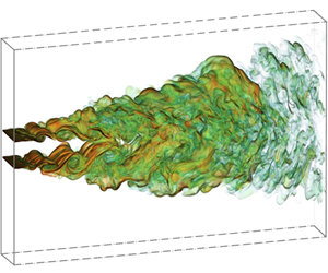
  $z=0$ plane at two representative instants; (c) volume rendering of
  $\text {FI} \times \log _{10}\text {HRR}$ at two representative instants. The exhibited region is
  $3\ \textrm {mm}< x<6\ \textrm {mm}, 0\ \textrm {mm}< y<2\ \textrm {mm}$ and
  $-1\ \textrm {mm}< z<1\ \textrm {mm}$. The upper halves of panel (a,b) were captured at the same instant, and the bottom halves of panel (a,b) were both captured at another instant. The left side of panel (c) was captured at the same instant as the upper panel of (b), and the right side was captured 0.9 ms later. Volume rendering was performed using VisIt (Childs et al. Reference Childs2012).
The flame could be observed to pass through three stages in the streamwise direction, described as follows:
(i) Upstream region with sparse autoignition kernels : As revealed by the contour of  $\chi$ in figure 2(a), large-scale vortices formed in the region of
  $x = 0 \sim 4H$ owing to jet shear effects. Within certain vortices, a few autoignition kernels formed at
  $x = 3 \sim 4H$, as annotated in figure 2(b). Consistent with the reports of previous studies on autoignition, these kernels formed in low-
 $\chi$ regions. This is because a low
  $\chi$ value indicates low loss of heat and radicals, which is conducive for the occurrence of autoignition. However, the findings of the current study and previous studies differed in terms of the location of these autoignition kernels in the
  $\xi$-space; previous studies on autoignition under ordinary conditions have reported that autoignition kernels usually form near
  $\xi _{MR}$ (Mastorakos et al. Reference Mastorakos, Baritaud and Poinsot1997; Mastorakos Reference Mastorakos2009). For the autoignition of supercritical hydrothermal flames in the current configuration (including the same pressure, fuel composition, oxidizer and fuel temperature), the author's previous work demonstrated that no well-defined
  $\xi _{MR}$ existed and that
  $\tau _{ig,0}$ decreased with
  $\xi$ on the fuel-rich side (Song et al. Reference Song, Luo, Jin, Wang and Fan2019, Reference Song, Jin, Wang, Gao, Luo and Fan2020). A DNS of autoignition in a 2-D mixing layer (Song et al. Reference Song, Luo, Jin, Wang and Fan2019) indicated that autoignition kernels tended to form in the range of
  $\xi = 0.80 - 0.85$. In contrast, the upstream autoignition kernels in the current simulation formed on the very fuel-lean side.
For turbulent jet flames in heated coflow, autoignition kernels are preferably favoured in the interior of large-scale shear-driven vortices on the fuel-lean side with a low scalar dissipation rate  $\chi$. The
  $\chi$ is always relatively large which suppresses ignition in the fuel-rich side. Under the current hydrothermal flame conditions, the ignition delay time
  $\tau _{ig,0}$ decreases quickly with the increase of mixture fraction in the fuel-rich side. However, the heat release rate is relative low in the very-fuel-rich mixture, where significant losses of heat and radicals occur owing to large
  $\chi$. Thus, there is a lack of ignition kernel formation on the fuel-rich side of the flow stream.
Figure 3 displays this upstream region in greater detail, which includes the contours of  $Y_{H_2}$,
  $Y_{O_2}$ and
  $T$, and a quiver plot of
  ${\boldsymbol{V}}$. The vortex-induced entrainment was observed to cause the direct transfer of
  $\textrm {H}_2$ from the jet core region to the centre of the vortices on the fuel-lean side. The interior of these vortices exhibited well-mixed fuel (
 $\textrm {H}_2$) and oxidant (
 $\textrm {O}_{2}$) along with low
  $\chi$ and velocity (figure 3d). Therefore, this region is favourable for the development of preignition chemistry and the occurrence of autoignition. Furthermore, as indicated by the contour of
  $T$ in figure 3(c), the recirculation of downstream flames did not involve the transport of hot combustion products into the upstream region. Therefore, in this simulation, autoignition was not triggered by the recirculation of hot combustion products. Thus, we can preliminarily conclude that these ignition kernels in the upstream region, which tend to form in the interior of large-scale shear-driven vortices on the fuel-lean side, are spontaneous ignition kernels and are significantly affected by flow structure and mixing history. This is consistent with the experimental observation that the increased turbulence would enhance mixing between the fuel and air streams and presumably lead to an earlier incipient flame formation (Hicks et al. Reference Hicks, Hegde and Kojima2019).

Figure 3. Snapshots of key variables on the  $z=0$ plane captured at the same instance as the upper panel of figure 2. The exhibited region is
  $0\ \textrm {mm}< x<5\ \textrm {mm}, 0\ \textrm {mm}< y<2\ \textrm {mm}$: (a) contour of
  $Y_{H_2}$; (b) contour of
  $Y_{O_2}$; (c) contour of
  $T$; (d) quiver plot of
  $\boldsymbol {V}$.
Figure 2(b) presents a time series of the contours of  $\text {FI} \times \text {HRR}$ in the subregion marked by a red box in the figure, which illustrates the evolution of the autoignition kernel in this upstream region. The ignition kernel evolved as the ignition front and moved downstream. During this evolution process, the ignition front remained in the premixed combustion mode. Volume rendering of
  $\text {FI} \times \log _{10}\text {HRR}$ (figure 2c) further confirmed that the premixed combustion mode was retained in all three dimensions. Studies on autoignition under ordinary conditions (Markides & Mastorakos Reference Markides and Mastorakos2005; Kerkemeier et al. Reference Kerkemeier, Markides, Frouzakis and Boulouchos2013) have reported that autoignition kernels rapidly transition to individual edge flames, which resemble triple flames composed of one non-premixed branch near
  $\xi _{st}$ and two premixed branches on the fuel-lean side and the fuel-rich side, respectively. For the autoignition of supercritical hydrothermal flames in a 2-D mixing layer (Song et al. Reference Song, Luo, Jin, Wang and Fan2019), the autoignition kernels transition to bibrachial edge flames composed of one non-premixed branch near
  $\xi _{st}$ and one premixed branch on the fuel-lean side. However, for the current flame, these autoignition kernels in the upstream region did not transition to multibrachial edge flames. This may be because these kernels formed in the interior of large-scale vortices and because the surrounding mixtures were relatively homogenous. These kernels were located far from the isosurfaces of
  $\xi _{st}$. The boundaries of the vortices, characterized by high
  $\chi$ values, also prevented the propagation of the ignition fronts to
  $\xi _{st}$. Notably, the sparsity of these kernels prevented their establishment of a continuous flame surface.
(ii) Middle region with intense ignition : As indicated in figure 2 for the downstream region, in the region  $x = 4 - 6 H$, the increase in
  $\chi$ owing to jet shear effects gradually tapered off and large-scale vortices separated into smaller vortices. In contrast to the sparse autoignition kernels observed in the upstream region, the downstream region exhibited dense and broadly distributed ignitions. These ignitions were still primarily in the premixed combustion mode and mainly distributed on the fuel-lean side. This region had a greater likelihood of ignitions than did the upstream region because of three possible reasons: a longer flow time, enabling the development of preignition chemistry and autoignition; lower
  $\chi$ values; and generation of hot combustion products from upstream autoignition kernels. These intense ignitions established a continuous flame surface, represented by the contour of
  $T$ in this region in figure 4. In the streamwise direction for the moment captured in figure 4, assessments conducted on the basis of the isoline of
  $T = 1200\ \textrm {K}$ revealed that the continuous flame surface began at approximately
  $x=4.6H$. A certain ignition process similar to the autoignition of supercritical hydrothermal flames in the 2-D mixing layer (Song et al. Reference Song, Luo, Jin, Wang and Fan2019) was occasionally observed to occur near
  $\xi _{st}$, as annotated in figure 2(b). This was because of the randomness of ignition occurrence; this kernel was observed near
  $\xi _{st}$ and could trigger the non-premixed branch. Statistical and quantitative analyses of the ignition process in this region and its differences from the upstream autoignition process are discussed in the following sections.

Figure 4. Snapshots of  $T$ on the
  $z=0$ plane captured at the same time as those displayed in the upper halves of figure 2(a,b). The exhibited region is
  $3\ \textrm {mm}< x<8\ \textrm {mm}, 0\ \textrm {mm}< y<3\ \textrm {mm}$. The dashed black lines represent the isolines of
  $T=1200\ \textrm {K}$.
(iii) Downstream region with massive flamelets : As revealed in figure 2(a,b), the isoline of  $\xi = \xi _{st}$ ended at approximately
  $x = 6H$. Further downstream, in the region of
  $x > 6H$, the isolines of
  $\xi = \xi _{st}$ formed several isolated and distributed islands, where a high HRR could be observed. In this region, the ratio of non-premixed HRR increased significantly. Quantitative analysis was subsequently conducted, as detailed in the following sections.
3.2. Statistical analysis of flame development
The flame structure and multistage characteristics are briefly outlined in § 3.1. The current section offers further discussion based on statistical and quantitative analyses.
First, the degree of mixing at various streamwise locations is discussed on the basis of the p.d.f.s of  $\xi$,
  $p_x(\xi )$. Samples were extracted along
  $y = 0.45H$ at various streamwise locations. Figure 5(a) presents the p.d.f. of
  $\xi$ at
  $x = 1H - 8H$, and figure 5(c) displays the Reynolds average and root-mean-square (r.m.s.) of
  $\xi$ in physical space (
 $\bar {\xi }$ and
  $\xi ^{\prime }$, respectively). The
  $\xi$-conditional Favre-averaged HRR,
  $\langle HRR | \xi \rangle$, was also calculated, as presented in figure 5(b), to characterize the distribution of mean combustion strength in
  $\xi$ space at various streamwise locations. The
  $\xi$-conditional Favre-averaged
  $\langle \phi | \xi \rangle$ of a scalar field variable
  $\phi$ can be calculated as follows (Yoo et al. Reference Yoo, Sankaran and Chen2009):
 \begin{equation} \langle \phi | \xi \rangle = \frac{\iiint (\rho \phi)|\xi\,\textrm{d}y\,\textrm{d}z\,\textrm{d}t}{\iiint \rho|\xi\,\textrm{d}y\,\textrm{d}z\,\textrm{d}t}. \end{equation}
Figure 5. Statistical analysis of the mixing degree at various streamwise locations: (a) profiles of the p.d.f.s of  $\xi$; (b) profiles of the
  $\xi$-conditional Favre-averaged HRR; (c) contour of the Reynolds average and r.m.s. of
  $\xi$ in physical space. The same colour bar is used for the contours of the Reynolds r.m.s. and Reynolds average of
  $\xi$.
At  $x=1H$,
  $p_x(\xi )$ peaked near
  $\xi = 1.0$. At
  $x=2H$,
  $p_x(\xi )$ exhibited a local peak at
  $\xi \approx 0.5$ owing to the mixing effect caused by large-scale shear vortices. No significant
  $\langle HRR | \xi \rangle$ was apparent at
  $x < 2H$, as indicated in figure 5(b). At
  $x=3H$,
  $p_x(\xi =0.5)$ and
  $p_x(\xi =1.0)$ had similar values, which indicated the presence of well-mixed mixtures on the fuel-lean side. The
  $\langle HRR | \xi \rangle$ was observed to span a wide range on the fuel-lean side, which corresponded to the HRR, primarily as a result of preignition chemistry and also possibly because of autoignition kernels. In the downstream region, the
  $p_x(\xi )$ peak on the fuel-lean side surpassed the peak on the fuel-rich side. At
  $x=4H$,
  $\langle HRR | \xi \rangle$ peaked at
  $\xi =0.6,$ with an approximate value of
  $1.5 \times 10^{10}\ \textrm {W}\ \textrm {m}^{-3}$. In regions further downstream, the
  $\langle HRR | \xi \rangle$ peak moved towards
  $\xi _{st}$, with higher values. As illustrated in figure 5(c), the isoline of
  $\bar {\xi } = \xi _{st}$ ended at approximately
  $x=4H$. As displayed by the transient contour in figure 2(b), the isoline of
  $\xi = \xi _{st}$ ended at approximately
  $x=6H$ because of the considerable fluctuations of
  $\xi$, as apparent in the contour of
  $\xi ^{\prime }$ in figure 5(c). High
  $\xi ^{\prime }$ values originated from the jet shear layer and expanded across an extensive area in regions further downstream.
The distribution of  $\text {FI} \times \text {HRR}$ was qualitatively investigated, as presented in § 3.1. To quantitatively analyse the distribution of HRR in
  $\xi$ space simultaneously in different combustion modes, the joint p.d.f. of
  $\text {FI} \times \log _{10}\text {HRR}$ and
  $\xi$,
  $p_x(\xi , \text {FI} \times \log _{10}\text {HRR})$ was calculated for various streamwise locations. The samples were extracted from the DNS results, which were filtered using a cutoff of
  $\textrm {HRR} > 1.0 \times 10^{11}\ \textrm {W}\ \textrm {m}^{-3}$. The results obtained for
  $p_x(\xi , \text {FI} \times \log _{10}\text {HRR})$ at
  $x=3H, 4H, 5H, 6H, 7H,\ \text {and}\ 9H$ are presented in figure 6. A transient contour of
  $\text {FI} \times \text {HRR}$ is also provided for convenience of reference and to aid discussion.

Figure 6. Joint p.d.f. of  $\xi$ and the combined field variable
  $\text {FI} \times \log _{10}\text {HRR}$ at various streamwise locations. The vertical black dashed line in each panel marks
  $\xi _{st}=0.911$. The univariate p.d.f.s of the two variables were also estimated and drawn on the marginal axes. For convenience of reference, a transient contour of
  $\text {FI} \times \text {HRR}$ is also presented.
At  $x=3H$, a high HRR was observed near
  $\xi = 0.5$, predominately in the premixed combustion mode. The estimation of
  $p_x(\xi , \text {FI}\times \log _{10}\text {HRR})$ was relatively rough owing to the small number of samples (with high HRR) at this location. At
  $x=4H$, we obtained a smooth estimation of
  $p_x(\xi , \text {FI}\times \log _{10}\text {HRR})$. At this location, high HRR values were mainly distributed in the range of
  $\xi = 0.45 - 0.65$, with a peak at approximately
  $\xi = 0.60$. No significantly high HRR values were observed on the fuel-rich side. In combination with the transient analysis results reported in § 3.1, these findings indicate that the HRR in the upstream region is attributable to the formation of autoignition kernels and subsequent ignition fronts. Through statistical analysis, these upstream autoignition kernels can be further concluded to form primarily in the premixed combustion mode. At
  $x=5H\ \text {and}\ 6H$, which corresponds to the middle region with intense ignitions , the distribution of high HRR values expanded towards
  $\xi _{st}$, and the proportion of non-premixed combustion increased. At
  $x=6H$, high HRR values could be observed at
  $\xi _{st}$ and the fuel-rich side. Further downstream, at
  $x=7H$ and
  $9H$, the HRR near
  $\xi _{st}$ could be seen to increase significantly, with the flame gradually becoming dominated by the non-premixed combustion mode.
The transient contour of  $T$ was obtained, and a preliminary inspection of the distribution of
  $T$ in figures 3(c) and 4 was performed. The highest temperature of this flame was
  $T_{max} = 1430\ \textrm {K}$. In figure 7, the
  $\xi$-conditional Favre average and variance of
  $T$ (
$T$ ( $\langle T | \xi \rangle$ and
  $G_{TT}^{1/2}$, respectively) are presented to investigate the statistical characteristics of
  $T$ in
  $\xi$ space at various streamwise locations. Here,
  $\langle T | \xi \rangle$ was calculated using (3.2) and
  $G_{TT}$ was calculated as follows (Yoo et al. Reference Yoo, Sankaran and Chen2009):
 \begin{equation} G_{\phi\phi} = \langle \phi^{\prime\prime}\phi^{\prime\prime} | \xi \rangle, \end{equation}
where  $\phi ^{\prime \prime }$ is the Favre fluctuation of
  $\phi$, calculated as
  $\phi ^{\prime \prime } = \phi - \langle \phi | \xi \rangle$.

Figure 7. Profiles of the  $\xi$-conditional Favre average and variance of
  $T$ at various streamwise locations.
At  $x=3H$,
  $\langle T | \xi \rangle$ exhibited almost no increase, but
  $G_{TT}^{1/2}$ had a peak value of approximately 25 K over an extensive area in
  $\xi$ space on the fuel-lean side. At
  $x=4H$,
  $\langle T | \xi \rangle$ increased slightly and
  $G_{TT}^{1/2}$ peaked at
  $\xi = 0.6$, with a value of 100 K. This region corresponds to the upstream region with sparse autoignition kernels introduced in § 3.1. The statistical characteristics of
  $T$ were consistent with the autoignition behaviour because these kernels were sparse and randomly distributed on the fuel-lean side. At
  $x=4H$, both
  $\langle T | \xi \rangle$ and
  $G_{TT}^{1/2}$ increased significantly on the fuel-lean side. For
  $x \geq 7H$, in areas further downstream, the
  $\langle T | \xi \rangle$ and
  $G_{TT}^{1/2}$ peaks moved towards
  $\xi _{st}$.
3.3. Characteristics of preignition chemistry and the fuel-rich side
The preceding sections focus primarily on high-temperature ignition and flames. For the current configuration of supercritical hydrogen hydrothermal flames (in terms of fuel composition, oxidizer, temperature and pressure conditions), the author's previous research on 0-D homogeneous autoignition, laminar non-premixed flames and autoignition in 2-D mixing layers indicated differences in preignition chemistry and reactions on the fuel-rich side compared with those of autoignition under ordinary conditions, as mentioned in § 1.3. The current study investigated these topics with respect to a 3-D supercritical hydrothermal flame in a slot jet; this investigation is described in this section.
Figure 8 presents the transient contour of  $Y_{H_2O_2}$ and the mass production rate of
  $\textrm {H}_2\textrm {O}_{2}$ radicals (
 $\dot {\omega }_{H_2O_2}$) at the same instant as that displayed in the upper half of figure 2(b). Notably, in figure 8, the bottom half for the contour of
  $\dot {\omega }_{H_2O_2}$ is flipped vertically to combine with the contour of
  $Y_{H_2O_2}$ for the convenience of integrated analysis. At
  $x \approx 2.5H$,
  $\textrm {H}_2\textrm {O}_{2}$ radicals exhibited a significant increase in production rate (mainly by R
 $13\,(\textrm {HO}_2+\textrm {HO}_2 \rightarrow \textrm {H}_2\textrm {O}_2+\textrm {O}_2)$) and accumulated in the interior of large-scale shear-driven vortices near the isoline of
  $\xi = 0.3$. At
  $x \approx 3.2H$, where upstream autoignition kernels formed,
  $\textrm {H}_2\textrm {O}_{2}$ radicals were consumed on the fuel-lean side mainly via R
 $14\,(\textrm {H}_2\textrm {O}_2 \rightarrow \textrm {OH}+\textrm {OH})$. Up to this location, the preignition chemistry was mainly observed on the fuel-lean side, consistent with the occurrence of autoignition kernels. Although the chemical time scale is shorter on the fuel-rich side (Song et al. Reference Song, Luo, Jin, Wang and Fan2019), because of the effects of the shear-driven flow structure, no clear signs of chemical reactions were observed in these regions. Between the upstream region with sparse autoignition kernels and the middle region with intense ignitions , a considerable quantity of
  $\textrm {H}_2\textrm {O}_{2}$ radicals was produced at a high concentration, with
  $\xi$ ranging from 0.3 to
  $\xi _{st}$, which led to the intense ignitions observed in the middle region. In the downstream region, the consumption of
  $\textrm {H}_2\textrm {O}_{2}$ radicals primarily occurred on the fuel-lean side, and the production of
  $\textrm {H}_2\textrm {O}_{2}$ radicals occurred inside the islands formed by the isoline of
  $\xi _{st}$ on the fuel-rich side.

Figure 8. Contour of the mass fraction and mass production rate of  $\textrm {H}_2\textrm {O}_{2}$ radicals (
 $Y_{H_2O2}$ and
  $\dot {\omega }_{H_2O_2}$, respectively). The contour of
  $\dot {\omega }_{H_2O_2}$ is flipped vertically to combine with the contour of
  $Y_{H_2O_2}$ for the convenience of integrated analysis.
Figure 9 displays the joint p.d.f. of  $\dot {\omega }_{H_2O_2}$ and
  $\xi$,
  $p_x(\xi , \dot {\omega }_{H_2O_2}$) at various streamwise locations; the derived p.d.f was used to statistically investigate the preignition chemistry. Consistent with the results in figure 8, at
  $x=2.5H$ and
  $x=4.0H$,
  $\textrm {H}_2\textrm {O}_{2}$ radicals exhibited a moderate production rate on the fuel-lean side, and the p.d.f. of
  $\dot {\omega }_{H_2O_2}$ peaked at
  $\xi \approx 0.6$. A larger half-width of
  $p_x(\dot {\omega }_{H_2O_2})$ was observed at
  $x=4.0H$ compared with that observed at
  $x=2.5H$, which statistically confirmed the occurrence of intense preignition chemistry before the middle region. In the downstream region, at
  $x=6.0H$ and
  $x=7.0H$,
  $\textrm {H}_2\textrm {O}_{2}$ radicals exhibited clear signs of production on the fuel-rich side; the consumption of
  $\textrm {H}_2\textrm {O}_{2}$ radicals mainly occurred on the fuel-lean side. In further downstream regions, at
  $x=9.0H$ and
  $x=10.0H$, the dominant reactivity of the preignition chemistry gradually moved to the fuel-rich side.

Figure 9. Joint p.d.f. of  $\xi$ and
  $\dot {\omega }_{H_2O_2}$ at various streamwise locations. The vertical black dashed line in each panel marks
  $\xi _{st}=0.911$. Estimates of the univariate p.d.f. of the two variables are also displayed on the marginal axes.
Figure 10 shows the  $\xi$-conditional Favre-averaged and variance of
  $Y_{OH}$ at various streamwise locations. It is observed that in the upstream region (
 $x = 3.0 \sim 4.0H$), the Favre average of
  $Y_{OH}$ is almost zero in the whole
  $\xi$ space, but for the variance of
  $Y_{OH}$, a moderate amount of radical
  $\textrm {OH}$ (
 ${\sim }5.0\times 10^{-6}$ ) can be observed to form in the fuel-lean side. The production of radical
  $\textrm {OH}$ mainly arises from the consumption of
  $\textrm {H}_2\textrm {O}_{2}$ radicals through R
 $14\,(\textrm {H}_2\textrm {O}_2 \rightarrow \textrm {OH}+\textrm {OH})$.

Figure 10. Profiles of the  $\xi$-conditional Favre average and variance of
  $Y_{OH}$ at various streamwise locations.
4. Autoignition characteristics
This section focuses on a comprehensive exploration of the characteristics of autoignition in the supercritical hydrothermal flame discussed in this study. Section 3 provides an overview of the flame structure and reveals the occurrence of multistage ignition in these flames. The inconsistency between the flame in the present study and autoignited flames investigated in previous studies regarding the location of autoignition kernel formation is discussed. The effects of flow structure were preliminarily investigated according to the transient contour of  $\chi$.
Figure 11 presents the joint p.d.f. of  $\chi$ and
  $\xi$ at various streamwise locations, with the profiles of
  $\langle \chi |\xi \rangle$ against
  $\xi$ also plotted in the corresponding panels. In the upstream region (
 $x = 2.5H$ and
  $3.5H$), the profiles of
  $\langle \chi |\xi \rangle$ exhibited two peaks, located at
  $\xi = 0.30$ and
  $\xi = 0.80$. In addition to the distribution of
  $p_x(\xi , \chi )$ in figure 11 and the transient contour of
  $\chi$ in figure 2(a), these findings suggest that high
  $\chi$ values mainly appear at the edges of large-scale vortices. The local minimum of
  $\langle \chi |\xi \rangle$ appeared at
  $\xi = 0.60$. According to the distribution of
  $p_x(\xi , \chi )$, low
  $\chi$ mainly appeared over a wide range of
  $\xi$ near
  $\xi = 0.60$. These low-
 $\chi$ regions were determined to correspond to the interior of large-scale vortices, as displayed in figure 2(a). Therefore, the statistically low
  $\chi$ values on the extremely fuel-lean side and statistically high
  $\chi$ values near
  $\xi =0.80$ and
  $\xi _{st}$ indicate that the formation of preignition chemistry and autoignition kernels in the upstream region tended to occur on the extremely fuel-lean side instead of near
  $\xi =0.80$ (which was the preferred location for the formation of autoignition kernels in the 2-D mixing layer in the author's previous study). Similar analyses were performed to evaluate the middle region with intense ignitions, as exemplified by the distribution of
  $p_x(\xi , \chi )$ at
  $x = 5.0H$ and
  $7.0H$. In brief, statistical analysis of
  $\chi$ further confirmed that in the current flame configuration, flow structures significantly affected the autoignition characteristics and determined the location of autoignition kernels.

Figure 11. Joint p.d.f. of  $\xi$ and
  $\chi$ at various streamwise locations. The profile of
  $\langle \chi |\xi \rangle$ against
  $\xi$ is also plotted in the corresponding panels. The vertical black dashed line in each panel marks
  $\xi _{st}=0.911$. Estimates of the univariate p.d.f. of the two variables are also displayed on the marginal axes.
To quantitatively investigate the role of autoignition in this supercritical hydrothermal flame configuration, the dimensionless Damköhler number  $Da$ was calculated and comprehensively analysed. The
  $Da$ is defined as the ratio of the reaction term to the diffusion term for a certain species, which provides a measurement of the strength of autoignition relative to that of flame deflagration. The main combustion product, namely
  $\textrm {H}_2\textrm {O}$, was selected as the main species for
  $Da$ evaluation:
 \begin{equation} Da = \frac{\dot{\omega}_k}{|-\partial/\partial x_j (\rho Y_k V_{j,k})|}, \end{equation}
where  $k$ denotes
  $\textrm {H}_2\textrm {O}$ species and
  $V_{j,k}$ denotes the diffusion velocity of the species in the
  $j$ direction. Here,
  $Da \gg 1$ typically indicates that local combustion is dominated by autoignition and
  $Da \approx 1$ typically denotes flame propagation.
Volume rendering was performed for the evaluation of  $Da$, as displayed in figure 12. The exhibited domain was as follows:
  $3.0\ \textrm {mm}< x<6.0\ \textrm {mm}$ and
  $0.0\ \textrm {mm}< y<2.0\ \textrm {mm}$. The domain encompassed both the upstream region with sparse autoignition kernels and the middle region with intense ignitions. The following two details should be noted: (i) the calculated
  $Da$ values spanned across a wide range (exceeding
  $1.0\times 10^{5}$) and were seldom high. Therefore, to qualitatively distinguish between regions dominated by autoignition and those dominated by flame propagation, the upper limit of the colour map in figure 12 is only 10.0, with the high-
 $Da$ region separately displayed; (ii) the transfer function for the volume rendering process, as shown in the colour bar of figure 12, was selected to highlight the
  $Da \approx 1.0$ region (in blue) and the high-
 $Da$ (
 $Da > 8$) region (in red). The application of these data visualization techniques revealed that high
  $Da$ values were distributed in small and discrete spherical regions, as illustrated in figure 12. For the upstream region containing autoignition kernels, several high-
 $Da$ spherical regions could be observed, which can be regarded as multiple ignition spots, surrounded by a continuous surface of
  $Da \approx 1$. For the middle region, a high density of ignition spots was observed, which confirmed the occurrence of autoignition near the flame base.

Figure 12. Volume rendering of  $Da$ with regions of
  $Da \approx 1$ and
  $Da > 8$ highlighted.
Figure 13 shows the joint p.d.f. of  $\log _{10} Da$ and
  $\xi$ at various streamwise locations; the p.d.f was used to statistically investigate the role of autoignition. To eliminate unreactive regions, the samples for the p.d.f. calculation were filtered from the DNS results using the following cutoff:
  $\textrm {HRR} > 1.0 \times 10^{11}\ \textrm {W}\ \textrm {m}^{-3}$. From
  $x=3.0H$ to
  $x=5.0H$ (i.e. from the upstream region with sparse autoignition to the middle region with intense ignitions),
  $p_x(\xi , \log _{10} Da)$ was observed to be primarily concentrated near
  $\xi \approx 0.6$, with a peak located slightly above zero (
 $Da>1$). With movement downstream to
  $x=6.0H, 8.0H$ and
  $10.0H$, the distribution of
  $p_x(\xi , \log _{10} Da)$ spread towards
  $\xi _{st}$ and
  $Da=1$. This indicates that in the downstream region, although high-
 $Da$ autoignition still occurred, local flame propagation is playing an increasingly important role and eventually becomes the dominant behaviour.

Figure 13. Joint p.d.f. of  $\xi$ and
  $\log _{10} Da$ at various streamwise locations. The vertical black dashed line in each panel marks
  $\xi _{st}=0.911$. The horizontal red dashed line in each panel marks
  $\log _{10} Da = 0$ (
 $Da=1$). Estimates of the univariate p.d.f. of the two variables are also displayed on the marginal axes.
The flame base of turbulent hydrothermal lifted flame is highly corrugated and strongly affected by the instantaneous local flow and mixture conditions. The liftoff height of the present hydrothermal flame can be marked by the averaged  $Y_{OH}$ (Yoo et al. Reference Yoo, Sankaran and Chen2009). The liftoff height is estimated as
  $H_L \approx 4.6H$ where the Favre average of
  $Y_{OH}$ reaches
  $5.0\times 10^{-6}$, as shown in figure 10 and the temperature contours in figure 4. For the autoignition stabilized flame, a basic prediction of the critical liftoff height is the balance of the flow time defined as
  $t_{flow} = H_L/U_j$ and the adiabatic ignition delay time
  $\tau _{ig,ad}$, and
  $H_L \approx U_j\tau _{ig,ad}$ (Choi, Kim & Chung Reference Choi, Kim and Chung2009). It works well in our previous simulation of a 2-D laminar diffusion flame, where
  $H_L \approx 2.52\ \textrm {mm}$ and
  $U_j\tau _{ig,ad}\approx 2.331\ \textrm {mm}$ (Song et al. Reference Song, Jin, Wang, Gao, Luo and Fan2020). For the present turbulent flame,
  $H_L \approx 4.6\ \textrm {mm}$ and
  $U_j\tau _{ig,ad}\approx 9.324\ \textrm {mm}$. Thus, turbulent mixing by the rollup of the shear-driven vortices, which favours autoignition and also promotes the flame stabilization.
The stabilization of the lifted jet flame is a highly localized phenomenon. Various theories have been proposed to explain the stabilization mechanism for turbulent lifted flames, which can be broadly categorized based on the premixedness of the mixture upstream of the flame base or the effect of local turbulence structure. For a turbulent lifted flame in heated coflow at temperature exceeding the ignition limit, autoignition was proposed to play an important role in the flame stabilization. It has been speculated that the flame stabilization in heated coflow was a consequence of the balance between consecutive autoignition events in hot fuel-lean mixtures and convection induced by the high-speed jet and coflow velocities (Yoo et al. Reference Yoo, Sankaran and Chen2009). In the present hydrothermal turbulent flame, autoignition kernels sparsely formed at the base of the lifted hydrothermal jet flame, which is affected by the rolling-up of the large-scale shear-driven vortices, as discussed in § 3.1. Furthermore, as revealed by the profiles of  $Da$, autoignition is dominant at the flame base, while local flame propagation gradually enhances and eventually dominates further downstream. Thus, it can be speculated that the flame stabilization at the base is mainly affected by autoignition, as well as the turbulent mixing by the shear-driven vortices.
5. Conclusions
This study conducted a 3-D DNS of an autoignited supercritical hydrothermal flame in a turbulent slot jet at 25.0 MPa; details regarding the mechanism of  $\textrm {H}_2/\textrm {O}_{2}$ reaction in SCW were used for the simulation. A numerical framework for modelling the real-fluid properties of multispecies was integrated with a low-Mach-number reactive flow solver, and qualitative and quantitative analyses were conducted to investigate the flame structure, combustion mode and autoignition characteristics.
The flame underwent a three-stage development process in the streamwise direction: sparse autoignition kernels in the upstream region, intense ignitions in the middle region, and massive flamelets in the downstream region. Transient inspection of the contour of the scalar dissipation rate  $\chi$ revealed that large-scale vortices formed in the upstream region owing to jet shear effects. A few sparse autoignition kernels randomly formed in the interior of the vortices (low
  $\chi$) on the fuel-lean side but did not establish a continuous flame surface. In the middle region, intense ignitions occurred primarily on the fuel-lean side, where the continuous flame surface began. An analysis of the joint p.d.f. of the combined field variable
  $\text {FI} \times \log _{10} (\textrm {HRR})$ and mixture fraction
  $\xi$ at various streamwise locations indicated that in the upstream and middle regions, combustion involving the autoignition process mainly occurred in the premixed combustion mode on the fuel-lean side (near
  $\xi =0.6$). The author's previous works indicated that no well-defined
  $\xi _{MR}$ exists for the current configuration and that autoignition kernels in a 2-D mixing layer tend to form in the
  $\xi$ range of 0.80–0.85 (stoichiometric mixture fraction
  $\xi _{st}=0.911$). However, in the current 3-D jet flame, ignition kernels primarily formed on the extremely fuel-lean side, a finding that could primarily be attributed to the effects of large-scale flow structures. In the downstream region, massive non-premixed flamelets were observed. The ratio of HRR in the non-premixed mode increased with movement further downstream, and the non-premixed mode gradually became the dominant combustion mode.
The characteristics of the preignition chemistry and fuel-rich side were investigated through qualitative and quantitative analyses of  $\textrm {H}_2\textrm {O}_{2}$ radicals. The author's previous studies on homogeneous autoignition characteristics have suggested that the fuel-rich side has a shorter autoignition time delay but a lower HRR. This feature is reflected by the bibrachial flame structure observed in previous studies on 2-D laminar flames and in the 2-D flame in the turbulent mixing layer, rather than the classic tribrachial flame structure. In the current 3-D jet flame, in the upstream and middle regions, no remarkably high HRR values or accumulation or production of
  $\textrm {H}_2\textrm {O}_{2}$ radicals were observed on the fuel-rich side. The current study revealed a high rate of
  $\textrm {H}_2\textrm {O}_{2}$ radical production on only the fuel-rich side and the rate increased with movement further downstream.
Autoignition characteristics were further investigated. The profiles of the  $\xi$-conditional Favre average of
  $\chi$,
  $\langle \chi | \xi \rangle$ in the upstream and middle regions exhibited a local minimum near
  $\xi =0.6$ and a global maximum at
  $\xi =0.8$. The joint p.d.f. of
  $\chi$ and
  $\xi$ indicated that in these regions, low
  $\chi$ values primarily occurred at
  $\xi <0.7$. Regions with
  $\xi >0.8$ mainly featured high
  $\chi$ values and were thus not favourable locations for the occurrence of autoignition. The dimensionless Damköhler number
  $Da$ was calculated and analysed to distinguish between local autoignition and flame propagation. Volume rendering of
  $Da$ was performed to elucidate the distribution of high-
 $Da$ regions (dominated by autoignition) and unity-
 $Da$ regions (dominated by flame propagation). The joint p.d.f. of
  $\log _{10} Da$ and
  $\xi$ statistically confirmed that autoignition occurred sparsely in the upstream region and densely in the middle region on the fuel-lean side. With movement downstream, the distribution of the joint p.d.f. of
  $\log _{10} Da$ and
  $\xi$ gradually spread towards
  $\xi _{st}$ and
  $Da=1$, which indicated the transition from autoignition to flame propagation. It can be speculated that the flame stabilization at the base is mainly affected by autoignition, as well as the turbulent mixing by the shear-driven vortices.
Funding
The authors gratefully acknowledge the financial support of the National Key Research and Development Program of China (No. 2016YFB0600102).
Declaration of interests
The authors report no conflict of interest.


