


1. Introduction
In the study of pure buoyancy-driven flow (natural convection) between two differentially heated vertical surfaces (figure 1
a), there has been an ongoing interest in establishing a general relationship between the heat transfer and the temperature difference for an arbitrary fluid. The heating and cooling that occurs in this vertical setup is a fundamental problem that is often found in applications such as building ventilation, computer systems and power plants. The relevant parameters are: the Nusselt number
 $\mathit{Nu}$
, that is, the dimensionless heat transfer rate; the Rayleigh number
$\mathit{Nu}$
, that is, the dimensionless heat transfer rate; the Rayleigh number
 $\mathit{Ra}$
, that is, the dimensionless temperature difference; and the Prandtl number
$\mathit{Ra}$
, that is, the dimensionless temperature difference; and the Prandtl number
 $\mathit{Pr}$
, that is, the ratio of fluid viscosity to the thermal diffusivity. Past studies have shown a preference for the power-law form,
$\mathit{Pr}$
, that is, the ratio of fluid viscosity to the thermal diffusivity. Past studies have shown a preference for the power-law form,
 $\mathit{Nu}\sim \mathit{Ra}^{p}$
(at fixed
$\mathit{Nu}\sim \mathit{Ra}^{p}$
(at fixed
 $\mathit{Pr}$
), but the exponent
$\mathit{Pr}$
), but the exponent
 $p$
has been reported to range anywhere between
$p$
has been reported to range anywhere between
 $1/3$
and
$1/3$
and
 $1/4$
(Batchelor Reference Batchelor1954; Elder Reference Elder1965; Churchill & Chu Reference Churchill and Chu1975; George & Capp Reference George and Capp1979; Tsuji & Nagano Reference Tsuji and Nagano1988; Versteegh & Nieuwstadt Reference Versteegh and Nieuwstadt1999; Kiš & Herwig Reference Kiš and Herwig2012; Ng, Chung & Ooi Reference Ng, Chung and Ooi2013). A careful examination of recent direct numerical simulation (DNS) data (figure 2) demonstrates this point: there is no range in which
$1/4$
(Batchelor Reference Batchelor1954; Elder Reference Elder1965; Churchill & Chu Reference Churchill and Chu1975; George & Capp Reference George and Capp1979; Tsuji & Nagano Reference Tsuji and Nagano1988; Versteegh & Nieuwstadt Reference Versteegh and Nieuwstadt1999; Kiš & Herwig Reference Kiš and Herwig2012; Ng, Chung & Ooi Reference Ng, Chung and Ooi2013). A careful examination of recent direct numerical simulation (DNS) data (figure 2) demonstrates this point: there is no range in which
 $\mathit{Nu}/\mathit{Ra}^{p}$
is constant and the effective power-law exponent depend on
$\mathit{Nu}/\mathit{Ra}^{p}$
is constant and the effective power-law exponent depend on
 $\mathit{Ra}$
and is less than
$\mathit{Ra}$
and is less than
 $1/3$
but greater than
$1/3$
but greater than
 $1/4$
. Thus, a pure power law may not be the best description of the heat-transfer relationship. One approach is a power-law fit of arbitrary exponent to the existing data (e.g.
$1/4$
. Thus, a pure power law may not be the best description of the heat-transfer relationship. One approach is a power-law fit of arbitrary exponent to the existing data (e.g.
 $p\approx 0.31$
in figure 2
a), but this ignores the underlying flow physics and is therefore risky when applied outside the range of calibration.
$p\approx 0.31$
in figure 2
a), but this ignores the underlying flow physics and is therefore risky when applied outside the range of calibration.
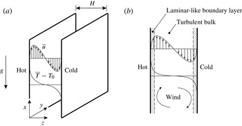
Figure 1. (a) Setup of vertical natural convection and (b) illustration of the laminar-like (boundary-layer) and turbulent (bulk) regions of the Grossmann–Lohse theory.
A similar scaling behaviour has also been reported in horizontal, i.e. Rayleigh–Bénard (RB), natural convection (e.g. Stevens, Lohse & Verzicco Reference Stevens, Lohse and Verzicco2011). In RB convection, the unifying theory of Grossmann & Lohse (Reference Grossmann and Lohse2000, Reference Grossmann and Lohse2001, Reference Grossmann and Lohse2002, Reference Grossmann and Lohse2004) (hereafter GL theory) offered a resolution to the previously experimentally found (Castaing et al.
Reference Castaing, Gunaratne, Heslot, Kadanoff, Libchaber, Thomae, Wu, Zaleski and Zanetti1989; Chavanne et al.
Reference Chavanne, Chillà, Castaing, Hébral, Chabaud and Chaussy1997, Reference Chavanne, Chillà, Chabaud, Castaing and Hebral2001) but unexplained
 $\mathit{Nu}\sim \mathit{Ra}^{0.289}$
behaviour (for unity
$\mathit{Nu}\sim \mathit{Ra}^{0.289}$
behaviour (for unity
 $\mathit{Pr}$
) by showing that the physics-unaware
$\mathit{Pr}$
) by showing that the physics-unaware
 $0.289$
-power can be understood as a combination of a
$0.289$
-power can be understood as a combination of a
 $1/4$
- and a
$1/4$
- and a
 $1/3$
-power-law scaling. The latter two exponents can be readily linked to distinct flow regimes. The GL theory works because it accounts for the possibility that, at moderate Rayleigh numbers and away from the walls, the buoyancy-driven turbulent ‘wind’ is not sufficiently strong to drive a turbulent boundary layer in the classical sense of Prandtl and von Kármán. The theory has since been further articulated and vetted by both experiments and simulations across a large range of
$1/3$
-power-law scaling. The latter two exponents can be readily linked to distinct flow regimes. The GL theory works because it accounts for the possibility that, at moderate Rayleigh numbers and away from the walls, the buoyancy-driven turbulent ‘wind’ is not sufficiently strong to drive a turbulent boundary layer in the classical sense of Prandtl and von Kármán. The theory has since been further articulated and vetted by both experiments and simulations across a large range of
 $\mathit{Ra}$
and
$\mathit{Ra}$
and
 $\mathit{Pr}$
(e.g. Ahlers, Grossmann & Lohse Reference Ahlers, Grossmann and Lohse2009; Stevens et al.
Reference Stevens, van der Poel, Grossmann and Lohse2013). The theory has also been extended to other related flows, including rotating RB convection (Stevens, Clercx & Lohse Reference Stevens, Clercx and Lohse2010a
) and Taylor–Couette flow (Eckhardt, Grossmann & Lohse Reference Eckhardt, Grossmann and Lohse2007). The success of the GL theory and the similarities between RB and vertical natural convection motivates the present study.
$\mathit{Pr}$
(e.g. Ahlers, Grossmann & Lohse Reference Ahlers, Grossmann and Lohse2009; Stevens et al.
Reference Stevens, van der Poel, Grossmann and Lohse2013). The theory has also been extended to other related flows, including rotating RB convection (Stevens, Clercx & Lohse Reference Stevens, Clercx and Lohse2010a
) and Taylor–Couette flow (Eckhardt, Grossmann & Lohse Reference Eckhardt, Grossmann and Lohse2007). The success of the GL theory and the similarities between RB and vertical natural convection motivates the present study.

Figure 2. Trend of
 $\mathit{Nu}$
versus
$\mathit{Nu}$
versus
 $\mathit{Ra}$
from recent DNS data for air (
$\mathit{Ra}$
from recent DNS data for air (
 $\mathit{Pr}=0.709$
): ▫, present simulations; ○, Versteegh & Nieuwstadt (Reference Versteegh and Nieuwstadt1999); ♢, Kiš & Herwig (Reference Kiš and Herwig2012). (a)
$\mathit{Pr}=0.709$
): ▫, present simulations; ○, Versteegh & Nieuwstadt (Reference Versteegh and Nieuwstadt1999); ♢, Kiš & Herwig (Reference Kiš and Herwig2012). (a)
 $\mathit{Nu}\sim \mathit{Ra}^{p}$
, where
$\mathit{Nu}\sim \mathit{Ra}^{p}$
, where
 $p\approx 0.31$
from a least-squares fit to a power law; (b) compensated form,
$p\approx 0.31$
from a least-squares fit to a power law; (b) compensated form,
 $\mathit{Nu}/\mathit{Ra}^{p}$
versus
$\mathit{Nu}/\mathit{Ra}^{p}$
versus
 $\mathit{Ra}$
. The trend exhibits neither a
$\mathit{Ra}$
. The trend exhibits neither a
 $1/4$
- nor a
$1/4$
- nor a
 $1/3$
-power scaling.
$1/3$
-power scaling.
In the following, we investigate a generalised application of the ideas of the GL theory to vertical natural convection through a close examination of the present DNS data (described in § 2) for
 $\mathit{Ra}=1.0\times 10^{5}$
–
$\mathit{Ra}=1.0\times 10^{5}$
–
 $1.0\times 10^{9}$
and
$1.0\times 10^{9}$
and
 $\mathit{Pr}=0.709$
. Many elements of the GL theory apply to vertical natural convection. Since the velocity is non-zero in the mean, the wind of the GL theory is readily identified and Prandtl–Blasius–Pohlhausen scaling of the boundary layers is easily verified (§ 3.1). The ‘bulk’ or ‘background’ flow regime (refer to figure 1
b) described by Kolmogorov–Obukhov–Corrsin scaling is also exhibited by the dissipation of turbulent fluctuations (§ 3.2). Apart from the obvious similarities, vertical natural convection is different to RB convection in one important respect: the horizontal direction of heat transfer in vertical natural convection is orthogonal to the vertical direction of the buoyancy flux, which is the source of turbulent kinetic energy. The heat flux and the buoyancy flux coincide in RB convection. Consequently, an exact relationship linking the global dissipation rate with
$\mathit{Pr}=0.709$
. Many elements of the GL theory apply to vertical natural convection. Since the velocity is non-zero in the mean, the wind of the GL theory is readily identified and Prandtl–Blasius–Pohlhausen scaling of the boundary layers is easily verified (§ 3.1). The ‘bulk’ or ‘background’ flow regime (refer to figure 1
b) described by Kolmogorov–Obukhov–Corrsin scaling is also exhibited by the dissipation of turbulent fluctuations (§ 3.2). Apart from the obvious similarities, vertical natural convection is different to RB convection in one important respect: the horizontal direction of heat transfer in vertical natural convection is orthogonal to the vertical direction of the buoyancy flux, which is the source of turbulent kinetic energy. The heat flux and the buoyancy flux coincide in RB convection. Consequently, an exact relationship linking the global dissipation rate with
 $\mathit{Nu}$
,
$\mathit{Nu}$
,
 $\mathit{Ra}$
and
$\mathit{Ra}$
and
 $\mathit{Pr}$
no longer exists (§ 3.3). However, it can be shown that the unclosed global-averaged buoyancy flux also exhibits both laminar and turbulent scaling behaviours, consistent with the GL theory. We conclude in § 4 by summarising current progress and speculate on future directions towards establishing closure for a generalised heat-transfer law for vertical natural convection.
$\mathit{Pr}$
no longer exists (§ 3.3). However, it can be shown that the unclosed global-averaged buoyancy flux also exhibits both laminar and turbulent scaling behaviours, consistent with the GL theory. We conclude in § 4 by summarising current progress and speculate on future directions towards establishing closure for a generalised heat-transfer law for vertical natural convection.
2. Flow setup and direct numerical simulations
2.1. Flow setup
We adopt the Boussinesq approximation in which density fluctuations are small relative to the mean. In this incompressible-flow approximation, the density fluctuation, which is linearly related to the temperature fluctuation, is dynamically significant only through the buoyancy force. The temperature difference,
 ${\rm\Delta}T=T_{h}-T_{c}$
, between the hot and cold bounding walls drives the fully developed turbulent natural convection (figure 1
a). The walls are separated by the distance
${\rm\Delta}T=T_{h}-T_{c}$
, between the hot and cold bounding walls drives the fully developed turbulent natural convection (figure 1
a). The walls are separated by the distance
 $H$
. The governing continuity, momentum and energy equations are respectively given by
$H$
. The governing continuity, momentum and energy equations are respectively given by
 $$\begin{eqnarray}\displaystyle & \displaystyle {\displaystyle \frac{\partial u_{i}}{\partial x_{i}}}=0, & \displaystyle\end{eqnarray}$$
 $$\begin{eqnarray}\displaystyle & \displaystyle {\displaystyle \frac{\partial u_{i}}{\partial t}}+u_{j}{\displaystyle \frac{\partial u_{i}}{\partial x_{j}}}=-\frac{1}{{\it\rho}_{0}}{\displaystyle \frac{\partial p}{\partial x_{i}}}+{\it\delta}_{i1}g{\it\beta}(T-T_{0})+{\it\nu}{\displaystyle \frac{\partial ^{2}u_{i}}{\partial x_{j}^{2}}}, & \displaystyle\end{eqnarray}$$
 $$\begin{eqnarray}\displaystyle & \displaystyle {\displaystyle \frac{\partial T}{\partial t}}+u_{j}{\displaystyle \frac{\partial T}{\partial x_{j}}}={\it\kappa}{\displaystyle \frac{\partial ^{2}T}{\partial x_{j}^{2}}}, & \displaystyle\end{eqnarray}$$
 $g$
is the gravitational acceleration,
$g$
is the gravitational acceleration,
 ${\it\beta}$
is the coefficient of thermal expansion,
${\it\beta}$
is the coefficient of thermal expansion,
 ${\it\nu}$
is the kinematic viscosity and
${\it\nu}$
is the kinematic viscosity and
 ${\it\kappa}$
is the thermal diffusivity, all assumed to be independent of temperature. The coordinate system
${\it\kappa}$
is the thermal diffusivity, all assumed to be independent of temperature. The coordinate system
 $x$
,
$x$
,
 $y$
and
$y$
and
 $z$
(or
$z$
(or
 $x_{1}$
,
$x_{1}$
,
 $x_{2}$
and
$x_{2}$
and
 $x_{3}$
) refers to the streamwise (opposing gravity), spanwise and wall-normal directions. The no-slip and no-penetration boundary conditions are imposed on the velocity at the walls. Periodic boundary conditions are imposed on
$x_{3}$
) refers to the streamwise (opposing gravity), spanwise and wall-normal directions. The no-slip and no-penetration boundary conditions are imposed on the velocity at the walls. Periodic boundary conditions are imposed on
 $u_{i}$
,
$u_{i}$
,
 $p$
and
$p$
and
 $T$
in the
$T$
in the
 $x$
- and
$x$
- and
 $y$
-directions. The Rayleigh, Nusselt and Prandtl numbers are respectively defined by
$y$
-directions. The Rayleigh, Nusselt and Prandtl numbers are respectively defined by  $$\begin{eqnarray}\displaystyle \mathit{Ra}\equiv \frac{g{\it\beta}{\rm\Delta}TH^{3}}{{\it\nu}{\it\kappa}},\quad \mathit{Nu}\equiv \frac{f_{w}\,H}{{\rm\Delta}T{\it\kappa}},\quad \mathit{Pr}\equiv \frac{{\it\nu}}{{\it\kappa}}, & & \displaystyle\end{eqnarray}$$
where
 $f_{w}\equiv {\it\kappa}|\text{d}\overline{T}/\text{d}z|_{w}$
is the wall heat flux and
$f_{w}\equiv {\it\kappa}|\text{d}\overline{T}/\text{d}z|_{w}$
is the wall heat flux and
 $(\cdot )|_{w}$
denotes the wall value. Here,
$(\cdot )|_{w}$
denotes the wall value. Here,
 $\overline{(\cdot )}$
denotes the spatial average in the
$\overline{(\cdot )}$
denotes the spatial average in the
 $xy$
-plane and
$xy$
-plane and
 $(\cdot )^{\prime }$
denotes the corresponding fluctuations.
$(\cdot )^{\prime }$
denotes the corresponding fluctuations.
Table 1. Simulation parameters of the present DNS cases.

2.2. Direct numerical simulations
In our simulations, the streamwise, spanwise and wall-normal domain sizes,
 $L_{x}\times L_{y}\times L_{z}$
, are
$L_{x}\times L_{y}\times L_{z}$
, are
 $8H\times 4H\times H$
and
$8H\times 4H\times H$
and
 $\mathit{Ra}=1.0\times 10^{5}$
–
$\mathit{Ra}=1.0\times 10^{5}$
–
 $1.0\times 10^{9}$
(table 1). The fluid is air with
$1.0\times 10^{9}$
(table 1). The fluid is air with
 $\mathit{Pr}=0.709$
. The present grid spacing is uniform in the
$\mathit{Pr}=0.709$
. The present grid spacing is uniform in the
 $x$
- and
$x$
- and
 $y$
-directions and is stretched by a cosine map in the
$y$
-directions and is stretched by a cosine map in the
 $z$
-direction in order to resolve the steep near-wall gradients. The resolutions are chosen so that the simulations resolve the Kolmogorov scale,
$z$
-direction in order to resolve the steep near-wall gradients. The resolutions are chosen so that the simulations resolve the Kolmogorov scale,
 ${\it\eta}\equiv [{\it\nu}^{3}/{\it\varepsilon}_{u^{\prime }}]^{1/4}$
, where
${\it\eta}\equiv [{\it\nu}^{3}/{\it\varepsilon}_{u^{\prime }}]^{1/4}$
, where
 ${\it\varepsilon}_{u^{\prime }}(z)\equiv {\it\nu}\overline{(\partial u_{i}^{\prime }/\partial x_{j})^{2}}$
is the turbulent dissipation. In the centre of the channel,
${\it\varepsilon}_{u^{\prime }}(z)\equiv {\it\nu}\overline{(\partial u_{i}^{\prime }/\partial x_{j})^{2}}$
is the turbulent dissipation. In the centre of the channel,
 ${\rm\Delta}_{x,y,z}<2.6{\it\eta}$
, while near the wall,
${\rm\Delta}_{x,y,z}<2.6{\it\eta}$
, while near the wall,
 ${\rm\Delta}_{x,y}<4.5{\it\eta}$
and
${\rm\Delta}_{x,y}<4.5{\it\eta}$
and
 ${\rm\Delta}_{z}<0.3{\it\eta}$
. With exception of the highest-
${\rm\Delta}_{z}<0.3{\it\eta}$
. With exception of the highest-
 $\mathit{Ra}$
case for which computational resources are limited, we report statistics averaged over at least
$\mathit{Ra}$
case for which computational resources are limited, we report statistics averaged over at least
 $400$
dimensionless turnover times, where a turnover time is defined by the free-fall period,
$400$
dimensionless turnover times, where a turnover time is defined by the free-fall period,
 $H/U_{{\rm\Delta}T}$
, where
$H/U_{{\rm\Delta}T}$
, where
 $U_{{\rm\Delta}T}\equiv (g{\it\beta}{\rm\Delta}TH)^{1/2}$
(cf. Stevens, Verzicco & Lohse Reference Stevens, Verzicco and Lohse2010b
). Higher-
$U_{{\rm\Delta}T}\equiv (g{\it\beta}{\rm\Delta}TH)^{1/2}$
(cf. Stevens, Verzicco & Lohse Reference Stevens, Verzicco and Lohse2010b
). Higher-
 $\mathit{Ra}$
cases are initialised using interpolated velocity and temperature fields from lower-
$\mathit{Ra}$
cases are initialised using interpolated velocity and temperature fields from lower-
 $\mathit{Ra}$
cases. Except for the highest-
$\mathit{Ra}$
cases. Except for the highest-
 $\mathit{Ra}$
case, the flow is first simulated for more than
$\mathit{Ra}$
case, the flow is first simulated for more than
 $70$
dimensionless turnover times in order to flush out transients before statistics are sampled. Throughout the sampling duration,
$70$
dimensionless turnover times in order to flush out transients before statistics are sampled. Throughout the sampling duration,
 $\mathit{Nu}$
remains within
$\mathit{Nu}$
remains within
 $5\,\%$
of its mean, which is sufficient to ensure a statistically stationary flow (Stevens et al.
Reference Stevens, Verzicco and Lohse2010b
). The switching between exponential growth in
$5\,\%$
of its mean, which is sufficient to ensure a statistically stationary flow (Stevens et al.
Reference Stevens, Verzicco and Lohse2010b
). The switching between exponential growth in
 $\mathit{Nu}$
due to the so-called elevator modes, followed by sudden breakdown, as observed in so-called homogeneous RB (Calzavarini et al.
Reference Calzavarini, Lohse, Toschi and Tripiccione2005, Reference Calzavarini, Doering, Gibbon, Lohse, Tanabe and Toschi2006; Schmidt et al.
Reference Schmidt, Calzavarini, Lohse, Toschi and Verzicco2012) is not observed in the present flow, as there is no destabilising mean vertical temperature gradient and the flow is bounded by plates. The DNS employs a fully conservative fourth-order staggered finite-difference scheme for the velocity field and the QUICK scheme to advect the temperature field. The equations are marched using a low-storage third-order Runge–Kutta scheme and fractional-step method for enforcing continuity at
$\mathit{Nu}$
due to the so-called elevator modes, followed by sudden breakdown, as observed in so-called homogeneous RB (Calzavarini et al.
Reference Calzavarini, Lohse, Toschi and Tripiccione2005, Reference Calzavarini, Doering, Gibbon, Lohse, Tanabe and Toschi2006; Schmidt et al.
Reference Schmidt, Calzavarini, Lohse, Toschi and Verzicco2012) is not observed in the present flow, as there is no destabilising mean vertical temperature gradient and the flow is bounded by plates. The DNS employs a fully conservative fourth-order staggered finite-difference scheme for the velocity field and the QUICK scheme to advect the temperature field. The equations are marched using a low-storage third-order Runge–Kutta scheme and fractional-step method for enforcing continuity at
 ${\rm\Delta}_{t}=\mathit{CFL}\,\max _{i}({\rm\Delta}_{i}/u_{i})$
, where we set
${\rm\Delta}_{t}=\mathit{CFL}\,\max _{i}({\rm\Delta}_{i}/u_{i})$
, where we set
 $\mathit{CFL}=1$
(for details, see Ng et al.
Reference Ng, Chung and Ooi2013; Ng Reference Ng2013). A zero-mass-flux constraint is enforced at every time step to improve convergence, which is similar to using top and bottom end walls (located far away) in an experiment (e.g. Elder Reference Elder1965).
$\mathit{CFL}=1$
(for details, see Ng et al.
Reference Ng, Chung and Ooi2013; Ng Reference Ng2013). A zero-mass-flux constraint is enforced at every time step to improve convergence, which is similar to using top and bottom end walls (located far away) in an experiment (e.g. Elder Reference Elder1965).
Comparisons of the present simulations with other DNS datasets (Versteegh & Nieuwstadt Reference Versteegh and Nieuwstadt1999; Pallares et al.
Reference Pallares, Vernet, Ferre and Grau2010; Kiš & Herwig Reference Kiš and Herwig2012) show good agreement for both mean and second-order statistics (figure 3). Throughout this study, statistics are averaged from both halves of the channel, taking the antisymmetry (about the centreline) of the mean profiles into account. The present simulations employ smaller periodic-domain sizes (two-thirds in each periodic direction) than the other DNS studies but are chosen in order to resolve the near-wall region at high
 $\mathit{Ra}$
. Simulations conducted with the larger periodic-domain sizes showed little difference in the mean and second-order statistics, which are the focus of the present study.
$\mathit{Ra}$
. Simulations conducted with the larger periodic-domain sizes showed little difference in the mean and second-order statistics, which are the focus of the present study.

Figure 3. Comparison of mean and second-order turbulent statistics from DNS for (a) velocity and (b) temperature, for
 $\mathit{Ra}=5.4\times 10^{5}$
: ——, present simulations; ○, Versteegh & Nieuwstadt (Reference Versteegh and Nieuwstadt1999);
$\mathit{Ra}=5.4\times 10^{5}$
: ——, present simulations; ○, Versteegh & Nieuwstadt (Reference Versteegh and Nieuwstadt1999);
 $\times$
, Pallares et al. (Reference Pallares, Vernet, Ferre and Grau2010); ♢, Kiš & Herwig (Reference Kiš and Herwig2012).
$\times$
, Pallares et al. (Reference Pallares, Vernet, Ferre and Grau2010); ♢, Kiš & Herwig (Reference Kiš and Herwig2012).
3. Results and discussion
The central idea in the GL theory is to conceptually split the flow into two regions: namely the boundary layer (or plume) and the bulk (or background) regions (Grossmann & Lohse Reference Grossmann and Lohse2000, Reference Grossmann and Lohse2001, Reference Grossmann and Lohse2004). Each of these regions contributes a distinct scaling behaviour to the total kinetic and thermal dissipations, as discussed in the following.

Figure 4. Definitions of the kinetic (
 ${\it\delta}_{u}$
) and thermal (
${\it\delta}_{u}$
) and thermal (
 ${\it\delta}_{T}$
) boundary-layer thicknesses shown for DNS data at
${\it\delta}_{T}$
) boundary-layer thicknesses shown for DNS data at
 $\mathit{Ra}=5.4\times 10^{5}$
(a,b) and
$\mathit{Ra}=5.4\times 10^{5}$
(a,b) and
 $\mathit{Ra}=2.0\times 10^{7}$
(c,d). The kinetic boundary layer is defined as the wall-distance to the intercept of
$\mathit{Ra}=2.0\times 10^{7}$
(c,d). The kinetic boundary layer is defined as the wall-distance to the intercept of
 $\overline{u}=\text{d}\overline{u}/\text{d}z|_{w}\,z$
and
$\overline{u}=\text{d}\overline{u}/\text{d}z|_{w}\,z$
and
 $\overline{u}=\overline{u}_{\mathit{max}}$
, and the thermal boundary layer is defined as the wall-distance to the intercept of
$\overline{u}=\overline{u}_{\mathit{max}}$
, and the thermal boundary layer is defined as the wall-distance to the intercept of
 $\overline{T}=T_{h}+\text{d}\overline{T}/\text{d}z|_{w}\,z$
and
$\overline{T}=T_{h}+\text{d}\overline{T}/\text{d}z|_{w}\,z$
and
 $\overline{T}=T_{\mathit{h}}-{\rm\Delta}T/2$
. These definitions roughly correspond to the crossover points between the mean dissipations and turbulent dissipations, i.e.
$\overline{T}=T_{\mathit{h}}-{\rm\Delta}T/2$
. These definitions roughly correspond to the crossover points between the mean dissipations and turbulent dissipations, i.e.
 $\overline{{\it\varepsilon}}_{\overline{u}}({\it\delta}_{u}^{d})=\overline{{\it\varepsilon}}_{u^{\prime }}({\it\delta}_{u}^{d})$
and
$\overline{{\it\varepsilon}}_{\overline{u}}({\it\delta}_{u}^{d})=\overline{{\it\varepsilon}}_{u^{\prime }}({\it\delta}_{u}^{d})$
and
 $\overline{{\it\varepsilon}}_{\overline{T}}({\it\delta}_{T}^{d})=\overline{{\it\varepsilon}}_{T^{\prime }}({\it\delta}_{T}^{d})$
.
$\overline{{\it\varepsilon}}_{\overline{T}}({\it\delta}_{T}^{d})=\overline{{\it\varepsilon}}_{T^{\prime }}({\it\delta}_{T}^{d})$
.

Figure 5. Trends of normalised boundary-layer thicknesses appear to scale with the
 $-1/2$
-power law of a wind-based Reynolds number. The boundary layer thicknesses are defined as: the distances to the intercepts (figure 4),
$-1/2$
-power law of a wind-based Reynolds number. The boundary layer thicknesses are defined as: the distances to the intercepts (figure 4),
 ${\it\delta}_{u}/H$
and
${\it\delta}_{u}/H$
and
 ${\it\delta}_{T}/H$
; the crossovers of dissipation profiles,
${\it\delta}_{T}/H$
; the crossovers of dissipation profiles,
 ${\it\delta}_{u}^{d}/H$
and
${\it\delta}_{u}^{d}/H$
and
 ${\it\delta}_{T}^{d}/H$
; and the displacement thickness,
${\it\delta}_{T}^{d}/H$
; and the displacement thickness,
 ${\it\delta}^{\ast }/H$
. Shown are the Prandtl–Blasius–Pohlhausen
${\it\delta}^{\ast }/H$
. Shown are the Prandtl–Blasius–Pohlhausen
 $-1/2$
-power scaling predictions for vertical natural convection (3.2a,b
) for
$-1/2$
-power scaling predictions for vertical natural convection (3.2a,b
) for
 ${\it\delta}_{T}$
(– – – -) and
${\it\delta}_{T}$
(– – – -) and
 ${\it\delta}_{u}$
(⋅ ⋅ ⋅ ⋅ ⋅ ⋅ ⋅). As reference, the laminar-to-turbulent transition of the shear boundary layer is expected to occur at
${\it\delta}_{u}$
(⋅ ⋅ ⋅ ⋅ ⋅ ⋅ ⋅). As reference, the laminar-to-turbulent transition of the shear boundary layer is expected to occur at
 $(\mathit{Re}_{{\it\delta}^{\ast }})_{\mathit{cr}}\approx 420$
(– ⋅ – ⋅ –) (Landau & Lifshitz Reference Landau and Lifshitz1987).
$(\mathit{Re}_{{\it\delta}^{\ast }})_{\mathit{cr}}\approx 420$
(– ⋅ – ⋅ –) (Landau & Lifshitz Reference Landau and Lifshitz1987).
3.1. Scaling of boundary-layer thicknesses
For moderate
 $\mathit{Ra}$
, the GL theory revealed that the kinetic and thermal boundary-layer thicknesses,
$\mathit{Ra}$
, the GL theory revealed that the kinetic and thermal boundary-layer thicknesses,
 ${\it\delta}_{u}$
and
${\it\delta}_{u}$
and
 ${\it\delta}_{T}$
, in fact obey a laminar-like Prandtl–Blasius–Pohlhausen scaling (cf. Landau & Lifshitz Reference Landau and Lifshitz1987):
${\it\delta}_{T}$
, in fact obey a laminar-like Prandtl–Blasius–Pohlhausen scaling (cf. Landau & Lifshitz Reference Landau and Lifshitz1987):
 $$\begin{eqnarray}\displaystyle {\it\delta}_{u}/H\sim \mathit{Re}^{-1/2},\quad {\it\delta}_{T}/H\sim \mathit{Re}^{-1/2}f(\mathit{Pr}),\quad \mathit{Re}\equiv UH/{\it\nu}, & & \displaystyle\end{eqnarray}$$
where
 $U$
refers to the wind. To test these predictions, we first need to define
$U$
refers to the wind. To test these predictions, we first need to define
 $U$
,
$U$
,
 ${\it\delta}_{u}$
and
${\it\delta}_{u}$
and
 ${\it\delta}_{T}$
for vertical natural convection. Unlike RB convection where the (mean) streamwise velocity is zero, the wind is readily identified for the vertical configuration because of the non-zero persistent (mean) streamwise velocity (see figure 1
a). Here, it is defined by
${\it\delta}_{T}$
for vertical natural convection. Unlike RB convection where the (mean) streamwise velocity is zero, the wind is readily identified for the vertical configuration because of the non-zero persistent (mean) streamwise velocity (see figure 1
a). Here, it is defined by
 $U=\overline{u}_{\mathit{max}}$
(figure 4
a,c). To define
$U=\overline{u}_{\mathit{max}}$
(figure 4
a,c). To define
 ${\it\delta}_{u}$
and
${\it\delta}_{u}$
and
 ${\it\delta}_{T}$
, we adopt definitions based on the gradient of the time- and plane-averaged velocity and temperature profiles at the wall (e.g. Zhou et al.
Reference Zhou, Stevens, Sugiyama, Grossmann, Lohse and Xia2010; Zhou & Xia Reference Zhou and Xia2010; Scheel & Schumacher Reference Scheel and Schumacher2014). The statistical properties of these definitions were also first systematically studied by Sun, Cheung & Xia (Reference Sun, Cheung and Xia2008). For the hot wall, the kinetic boundary-layer thickness,
${\it\delta}_{T}$
, we adopt definitions based on the gradient of the time- and plane-averaged velocity and temperature profiles at the wall (e.g. Zhou et al.
Reference Zhou, Stevens, Sugiyama, Grossmann, Lohse and Xia2010; Zhou & Xia Reference Zhou and Xia2010; Scheel & Schumacher Reference Scheel and Schumacher2014). The statistical properties of these definitions were also first systematically studied by Sun, Cheung & Xia (Reference Sun, Cheung and Xia2008). For the hot wall, the kinetic boundary-layer thickness,
 ${\it\delta}_{u}$
, is defined as the wall-normal distance to the intercept of
${\it\delta}_{u}$
, is defined as the wall-normal distance to the intercept of
 $\overline{u}=\text{d}\overline{u}/\text{d}z|_{w}\,z$
and
$\overline{u}=\text{d}\overline{u}/\text{d}z|_{w}\,z$
and
 $\overline{u}=U$
(figure 4
a,c), i.e.
$\overline{u}=U$
(figure 4
a,c), i.e.
 ${\it\delta}_{u}=U/(\text{d}\overline{u}/\text{d}z|_{w})$
, while the thermal boundary-layer thickness,
${\it\delta}_{u}=U/(\text{d}\overline{u}/\text{d}z|_{w})$
, while the thermal boundary-layer thickness,
 ${\it\delta}_{T}$
, is defined as the wall-normal distance to the intercept of
${\it\delta}_{T}$
, is defined as the wall-normal distance to the intercept of
 $\overline{T}=T_{h}+\text{d}\overline{T}/\text{d}z|_{w}\,z$
and
$\overline{T}=T_{h}+\text{d}\overline{T}/\text{d}z|_{w}\,z$
and
 $\overline{T}=T_{h}-{\rm\Delta}T/2$
(figure 4
b,d), i.e.
$\overline{T}=T_{h}-{\rm\Delta}T/2$
(figure 4
b,d), i.e.
 ${\it\delta}_{T}=-({\rm\Delta}T/2)/(\text{d}\overline{T}/\text{d}z|_{w})$
. These boundary-layer definitions conveniently distinguish the boundary-layer behaviour of the flow from the bulk behaviour and this is demonstrated for two representative
${\it\delta}_{T}=-({\rm\Delta}T/2)/(\text{d}\overline{T}/\text{d}z|_{w})$
. These boundary-layer definitions conveniently distinguish the boundary-layer behaviour of the flow from the bulk behaviour and this is demonstrated for two representative
 $\mathit{Ra}$
in figure 4. In figure 4(a,c), the kinetic dissipation due to the mean,
$\mathit{Ra}$
in figure 4. In figure 4(a,c), the kinetic dissipation due to the mean,
 $\overline{{\it\varepsilon}}_{\overline{u}}\equiv {\it\nu}\overline{(\partial \overline{u}_{i}/\partial x_{j})^{2}}={\it\nu}(\text{d}\overline{u}/\text{d}z)^{2}$
, overwhelms the kinetic dissipation due to the turbulent fluctuations,
$\overline{{\it\varepsilon}}_{\overline{u}}\equiv {\it\nu}\overline{(\partial \overline{u}_{i}/\partial x_{j})^{2}}={\it\nu}(\text{d}\overline{u}/\text{d}z)^{2}$
, overwhelms the kinetic dissipation due to the turbulent fluctuations,
 $\overline{{\it\varepsilon}}_{u^{\prime }}\equiv {\it\nu}\overline{(\partial u_{i}^{\prime }/\partial x_{j})^{2}}$
in the kinetic boundary layer. Similarly, in figure 4(b,d), the thermal dissipation due to the mean,
$\overline{{\it\varepsilon}}_{u^{\prime }}\equiv {\it\nu}\overline{(\partial u_{i}^{\prime }/\partial x_{j})^{2}}$
in the kinetic boundary layer. Similarly, in figure 4(b,d), the thermal dissipation due to the mean,
 $\overline{{\it\varepsilon}}_{\overline{T}}\equiv {\it\kappa}\overline{(\partial \overline{T}/\partial x_{j})^{2}}={\it\kappa}(\text{d}\overline{T}/\text{d}z)^{2}$
, overwhelms the thermal dissipation due to the turbulent fluctuations,
$\overline{{\it\varepsilon}}_{\overline{T}}\equiv {\it\kappa}\overline{(\partial \overline{T}/\partial x_{j})^{2}}={\it\kappa}(\text{d}\overline{T}/\text{d}z)^{2}$
, overwhelms the thermal dissipation due to the turbulent fluctuations,
 $\overline{{\it\varepsilon}}_{T^{\prime }}\equiv {\it\kappa}\overline{(\partial T^{\prime }/\partial x_{j})^{2}}$
, in the thermal boundary layer. Both profiles of
$\overline{{\it\varepsilon}}_{T^{\prime }}\equiv {\it\kappa}\overline{(\partial T^{\prime }/\partial x_{j})^{2}}$
, in the thermal boundary layer. Both profiles of
 $\overline{{\it\varepsilon}}_{u^{\prime }}$
and
$\overline{{\it\varepsilon}}_{u^{\prime }}$
and
 $\overline{{\it\varepsilon}}_{T^{\prime }}$
exhibit characteristics similar to that found in RB convection: the profiles peak at the wall and are approximately flat in the bulk (e.g. Emran & Schumacher Reference Emran and Schumacher2008; Kaczorowski & Wagner Reference Kaczorowski and Wagner2009; Kaczorowski & Xia Reference Kaczorowski and Xia2013). Alternative boundary-layer definitions such as the crossover locations between the mean dissipations and fluctuation dissipations,
$\overline{{\it\varepsilon}}_{T^{\prime }}$
exhibit characteristics similar to that found in RB convection: the profiles peak at the wall and are approximately flat in the bulk (e.g. Emran & Schumacher Reference Emran and Schumacher2008; Kaczorowski & Wagner Reference Kaczorowski and Wagner2009; Kaczorowski & Xia Reference Kaczorowski and Xia2013). Alternative boundary-layer definitions such as the crossover locations between the mean dissipations and fluctuation dissipations,
 ${\it\delta}_{u}^{d}$
and
${\it\delta}_{u}^{d}$
and
 ${\it\delta}_{T}^{d}$
, as well as the displacement thickness,
${\it\delta}_{T}^{d}$
, as well as the displacement thickness,
 ${\it\delta}^{\ast }\equiv \int _{0}^{{\it\delta}_{\mathit{max}}}(1-\overline{u}/\overline{u}_{\mathit{max}})\text{d}z$
, where
${\it\delta}^{\ast }\equiv \int _{0}^{{\it\delta}_{\mathit{max}}}(1-\overline{u}/\overline{u}_{\mathit{max}})\text{d}z$
, where
 $\overline{u}({\it\delta}_{\mathit{max}})=\overline{u}_{\mathit{max}}$
, are found to provide similar scaling characteristics, as verified in figure 5.
$\overline{u}({\it\delta}_{\mathit{max}})=\overline{u}_{\mathit{max}}$
, are found to provide similar scaling characteristics, as verified in figure 5.
For comparison, we compute the Prandtl–Blasius–Pohlhausen boundary-layer thicknesses for vertical natural convection from the laminar similarity scaling, which is different to its horizontal counterpart. Using the definitions for
 ${\it\delta}_{u}$
,
${\it\delta}_{u}$
,
 ${\it\delta}_{T}$
(figure 4) and wind-based
${\it\delta}_{T}$
(figure 4) and wind-based
 $\mathit{Re}$
from (3.1c
) and for
$\mathit{Re}$
from (3.1c
) and for
 $\mathit{Pr}=0.709$
, we obtain, by setting
$\mathit{Pr}=0.709$
, we obtain, by setting
 $x/H=1$
in the laminar similarity scaling (see White Reference White1991, §§ 4–13.3):
$x/H=1$
in the laminar similarity scaling (see White Reference White1991, §§ 4–13.3):
 $$\begin{eqnarray}\displaystyle {\it\delta}_{u}/H\approx 0.43\,\mathit{Re}^{-1/2},\quad {\it\delta}_{T}/H\approx 2.10\,\mathit{Re}^{-1/2}. & & \displaystyle\end{eqnarray}$$
Varying
 $x/H$
, pertaining to the wall-parallel coherence of the wind, would merely alter the coefficients in (3.2a,b
). In figure 5, the boundary-layer thicknesses using the slope definition from figure 4, i.e.
$x/H$
, pertaining to the wall-parallel coherence of the wind, would merely alter the coefficients in (3.2a,b
). In figure 5, the boundary-layer thicknesses using the slope definition from figure 4, i.e.
 ${\it\delta}_{u}$
and
${\it\delta}_{u}$
and
 ${\it\delta}_{T}$
, the dissipation crossover definitions,
${\it\delta}_{T}$
, the dissipation crossover definitions,
 ${\it\delta}_{u}^{d}$
and
${\it\delta}_{u}^{d}$
and
 ${\it\delta}_{T}^{d}$
, and displacement thickness
${\it\delta}_{T}^{d}$
, and displacement thickness
 ${\it\delta}^{\ast }$
, are compared with (3.2a,b
). Using a least-squares fit of the present data to a power law, we find that
${\it\delta}^{\ast }$
, are compared with (3.2a,b
). Using a least-squares fit of the present data to a power law, we find that
 ${\it\delta}_{u}/H\sim \mathit{Re}^{-0.45}$
and
${\it\delta}_{u}/H\sim \mathit{Re}^{-0.45}$
and
 ${\it\delta}_{T}/H\sim \mathit{Re}^{-0.60}$
(not shown in figure 5) which is in fair agreement with the
${\it\delta}_{T}/H\sim \mathit{Re}^{-0.60}$
(not shown in figure 5) which is in fair agreement with the
 $\mathit{Re}^{-1/2}$
trend, in accordance to the laminar predictions from the GL theory and past experimental results for RB convection (e.g. Sun et al.
Reference Sun, Cheung and Xia2008). Hence, for simplicity, we will adopt the boundary-layer definitions based on
$\mathit{Re}^{-1/2}$
trend, in accordance to the laminar predictions from the GL theory and past experimental results for RB convection (e.g. Sun et al.
Reference Sun, Cheung and Xia2008). Hence, for simplicity, we will adopt the boundary-layer definitions based on
 ${\it\delta}_{u}$
and
${\it\delta}_{u}$
and
 ${\it\delta}_{T}$
hereafter. An upper bound for the boundary layers can be obtained when both boundary-layer and bulk regions are laminar. In this case, the velocity profile is a cubic and the temperature profile is linear, from which
${\it\delta}_{T}$
hereafter. An upper bound for the boundary layers can be obtained when both boundary-layer and bulk regions are laminar. In this case, the velocity profile is a cubic and the temperature profile is linear, from which
 ${\it\delta}_{u}/H\approx 0.096$
and
${\it\delta}_{u}/H\approx 0.096$
and
 ${\it\delta}_{T}/H=0.5$
. For reference, the laminar-to-turbulent transition which occurs at
${\it\delta}_{T}/H=0.5$
. For reference, the laminar-to-turbulent transition which occurs at
 $(\mathit{Re}_{{\it\delta}^{\ast }})_{\mathit{cr}}\equiv (U{\it\delta}^{\ast }/{\it\nu})_{\mathit{cr}}\approx 420$
, where
$(\mathit{Re}_{{\it\delta}^{\ast }})_{\mathit{cr}}\equiv (U{\it\delta}^{\ast }/{\it\nu})_{\mathit{cr}}\approx 420$
, where
 ${\it\delta}^{\ast }$
is the displacement thickness (Landau & Lifshitz Reference Landau and Lifshitz1987), is also shown in figure 5, to the right of all the present data. Consistent with the insight provided by the GL theory, the boundary layers in vertical natural convection for the present
${\it\delta}^{\ast }$
is the displacement thickness (Landau & Lifshitz Reference Landau and Lifshitz1987), is also shown in figure 5, to the right of all the present data. Consistent with the insight provided by the GL theory, the boundary layers in vertical natural convection for the present
 $\mathit{Ra}$
range cannot be considered as turbulent boundary layers. Instead, they can be interpreted as laminar boundary layers animated by the turbulent wind.
$\mathit{Ra}$
range cannot be considered as turbulent boundary layers. Instead, they can be interpreted as laminar boundary layers animated by the turbulent wind.
Figure 5 shows that
 ${\it\delta}_{T}>{\it\delta}_{u}$
in all cases considered here at
${\it\delta}_{T}>{\it\delta}_{u}$
in all cases considered here at
 $\mathit{Pr}=0.709$
. This situation is expected to be reversed (
$\mathit{Pr}=0.709$
. This situation is expected to be reversed (
 ${\it\delta}_{u}>{\it\delta}_{T}$
) when
${\it\delta}_{u}>{\it\delta}_{T}$
) when
 $\mathit{Pr}>1$
(Grossmann & Lohse Reference Grossmann and Lohse2001). At transitional
$\mathit{Pr}>1$
(Grossmann & Lohse Reference Grossmann and Lohse2001). At transitional
 $\mathit{Ra}$
and at high
$\mathit{Ra}$
and at high
 $\mathit{Pr}$
, an oscillatory flow regime is found in vertical natural convection (Chait & Korpela Reference Chait and Korpela1989) and it remains unknown whether this oscillatory flow persists at higher
$\mathit{Pr}$
, an oscillatory flow regime is found in vertical natural convection (Chait & Korpela Reference Chait and Korpela1989) and it remains unknown whether this oscillatory flow persists at higher
 $\mathit{Ra}$
and whether (3.1b
) accounts for this behaviour.
$\mathit{Ra}$
and whether (3.1b
) accounts for this behaviour.
3.2. Boundary-layer and bulk contributions to the dissipations
The GL theory splits the global-averaged kinetic and thermal dissipation rates into contributions from the boundary layer and bulk regions (figure 1) such that
 $$\begin{eqnarray}\displaystyle & \displaystyle \langle {\it\varepsilon}_{u}\rangle =\langle {\it\varepsilon}_{u}\rangle _{BL}+\langle {\it\varepsilon}_{u}\rangle _{\mathit{bulk}}={\displaystyle \frac{2}{H}}\int _{0}^{{\it\delta}_{u}}{\it\nu}\left({\displaystyle \frac{\partial u_{i}}{\partial x_{j}}}\right)^{2}\text{d}z+{\displaystyle \frac{2}{H}}\int _{{\it\delta}_{u}}^{H/2}{\it\nu}\left({\displaystyle \frac{\partial u_{i}}{\partial x_{j}}}\right)^{2}\text{d}z, & \displaystyle\end{eqnarray}$$
 $$\begin{eqnarray}\displaystyle & \displaystyle \langle {\it\varepsilon}_{T}\rangle =\langle {\it\varepsilon}_{T}\rangle _{BL}+\langle {\it\varepsilon}_{T}\rangle _{\mathit{bulk}}={\displaystyle \frac{2}{H}}\int _{0}^{{\it\delta}_{T}}{\it\kappa}\left({\displaystyle \frac{\partial T}{\partial x_{j}}}\right)^{2}\text{d}z+{\displaystyle \frac{2}{H}}\int _{{\it\delta}_{T}}^{H/2}{\it\kappa}\left({\displaystyle \frac{\partial T}{\partial x_{j}}}\right)^{2}\text{d}z, & \displaystyle\end{eqnarray}$$
 $\langle \cdot \rangle$
. Following the GL theory, once the wind that acts on the boundary layer is identified as
$\langle \cdot \rangle$
. Following the GL theory, once the wind that acts on the boundary layer is identified as
 $U$
, the kinetic boundary-layer dissipation,
$U$
, the kinetic boundary-layer dissipation,
 $\langle {\it\varepsilon}_{u}\rangle _{BL}$
, is approximated using the wall-normal gradient of the streamwise velocity, i.e.
$\langle {\it\varepsilon}_{u}\rangle _{BL}$
, is approximated using the wall-normal gradient of the streamwise velocity, i.e.
 ${\it\nu}(\partial u_{i}/\partial x_{j})^{2}\approx {\it\nu}(U/{\it\delta}_{u})^{2}$
, over the volume fraction,
${\it\nu}(\partial u_{i}/\partial x_{j})^{2}\approx {\it\nu}(U/{\it\delta}_{u})^{2}$
, over the volume fraction,
 ${\it\delta}_{u}/H$
. Similarly, the thermal boundary-layer dissipation,
${\it\delta}_{u}/H$
. Similarly, the thermal boundary-layer dissipation,
 $\langle {\it\varepsilon}_{T}\rangle _{BL}$
, is approximated using the wall-normal gradient of the temperature, i.e.
$\langle {\it\varepsilon}_{T}\rangle _{BL}$
, is approximated using the wall-normal gradient of the temperature, i.e.
 ${\it\kappa}(\partial T/\partial x_{j})^{2}\approx {\it\kappa}({\rm\Delta}T/{\it\delta}_{T})^{2}$
, over the volume fraction
${\it\kappa}(\partial T/\partial x_{j})^{2}\approx {\it\kappa}({\rm\Delta}T/{\it\delta}_{T})^{2}$
, over the volume fraction
 ${\it\delta}_{T}/H$
. The boundary-layer terms on the right-hand side of (3.3a,b
) can thus be written as
${\it\delta}_{T}/H$
. The boundary-layer terms on the right-hand side of (3.3a,b
) can thus be written as  $$\begin{eqnarray}\displaystyle & \displaystyle \langle {\it\varepsilon}_{u}\rangle _{BL}\sim {\it\nu}\frac{U^{2}}{{\it\delta}_{u}^{2}}\left(\frac{{\it\delta}_{u}}{H}\right)\sim {\it\nu}\frac{U^{2}}{{\it\delta}_{u}^{2}}(\mathit{Re}^{-1/2})=\frac{{\it\nu}^{3}}{H^{4}}\mathit{Re}^{5/2}, & \displaystyle\end{eqnarray}$$
 $$\begin{eqnarray}\displaystyle & \displaystyle \langle {\it\varepsilon}_{T}\rangle _{BL}\sim {\it\kappa}\frac{{\rm\Delta}T^{2}}{{\it\delta}_{T}^{2}}\left(\frac{{\it\delta}_{T}}{H}\right)\sim {\it\kappa}\frac{{\rm\Delta}T^{2}}{{\it\delta}_{T}^{2}}(\mathit{Re}^{-1/2}f(\mathit{Pr}))={\it\kappa}{\displaystyle \frac{{\rm\Delta}T^{2}}{H^{2}}}\mathit{Re}^{1/2}f(\mathit{Pr}), & \displaystyle\end{eqnarray}$$
 ${\it\delta}_{u}/H$
and
${\it\delta}_{u}/H$
and
 ${\it\delta}_{T}/H$
in (3.1a,b
) are used. On the other hand, the bulk dissipation terms are modelled as
${\it\delta}_{T}/H$
in (3.1a,b
) are used. On the other hand, the bulk dissipation terms are modelled as  $$\begin{eqnarray}\displaystyle \langle {\it\varepsilon}_{u}\rangle _{\mathit{bulk}}\sim {\displaystyle \frac{U^{3}}{H}}={\displaystyle \frac{{\it\nu}^{3}}{H^{4}}}\mathit{Re}^{3},\quad \langle {\it\varepsilon}_{T}\rangle _{\mathit{bulk}}\sim {\displaystyle \frac{U{\rm\Delta}T^{2}}{H}}={\it\kappa}{\displaystyle \frac{{\rm\Delta}T^{2}}{H^{2}}}\mathit{Pr}\,\mathit{Re}, & & \displaystyle\end{eqnarray}$$
which follow from dimensional arguments of the turbulence cascade in the bulk region. In this region, larger eddies transfer energy to smaller eddies. Thus, the dissipation rate can be thought to scale with the largest eddies with energy of order
 $U^{2}$
and timescale
$U^{2}$
and timescale
 $H/U$
, independent of
$H/U$
, independent of
 ${\it\nu}$
. Similarly, the thermal dissipation rate can be thought to scale with the largest eddies with variance of order
${\it\nu}$
. Similarly, the thermal dissipation rate can be thought to scale with the largest eddies with variance of order
 ${\rm\Delta}T^{2}$
and timescale
${\rm\Delta}T^{2}$
and timescale
 $H/U$
, independent of
$H/U$
, independent of
 ${\it\kappa}$
(see Pope Reference Pope2000). Figure 6(a,b) shows the trends of the boundary-layer and bulk contributions. In figure 6(a), although
${\it\kappa}$
(see Pope Reference Pope2000). Figure 6(a,b) shows the trends of the boundary-layer and bulk contributions. In figure 6(a), although
 $\langle {\it\varepsilon}_{u}\rangle _{BL}\sim \mathit{Re}^{5/2}$
and
$\langle {\it\varepsilon}_{u}\rangle _{BL}\sim \mathit{Re}^{5/2}$
and
 $\langle {\it\varepsilon}_{u}\rangle _{\mathit{bulk}}\sim \mathit{Re}^{3}$
as predicted in (3.4a
) and (3.5a
), the ratio of boundary-layer-to-bulk contributions for thermal dissipation appears constant as shown by the parallel trends of
$\langle {\it\varepsilon}_{u}\rangle _{\mathit{bulk}}\sim \mathit{Re}^{3}$
as predicted in (3.4a
) and (3.5a
), the ratio of boundary-layer-to-bulk contributions for thermal dissipation appears constant as shown by the parallel trends of
 $\langle {\it\varepsilon}_{T}\rangle _{BL}$
and
$\langle {\it\varepsilon}_{T}\rangle _{BL}$
and
 $\langle {\it\varepsilon}_{T}\rangle _{\mathit{bulk}}$
in figure 6(b). This seemingly contradicts the
$\langle {\it\varepsilon}_{T}\rangle _{\mathit{bulk}}$
in figure 6(b). This seemingly contradicts the
 $\langle {\it\varepsilon}_{T}\rangle _{BL}\sim \mathit{Re}^{1/2}$
and
$\langle {\it\varepsilon}_{T}\rangle _{BL}\sim \mathit{Re}^{1/2}$
and
 $\langle {\it\varepsilon}_{T}\rangle _{\mathit{bulk}}\sim \mathit{Re}$
predictions for the boundary-layer and bulk thermal dissipations, (3.4b
) and (3.5b
). A similar behaviour is reported by Grossmann & Lohse (Reference Grossmann and Lohse2004) based on a DNS study of RB convection by Verzicco & Camussi (Reference Verzicco and Camussi2003). The reason is that plumes, which provide the scaling in (3.4b
), are also present in the bulk, as discussed in Grossmann & Lohse (Reference Grossmann and Lohse2004).
$\langle {\it\varepsilon}_{T}\rangle _{\mathit{bulk}}\sim \mathit{Re}$
predictions for the boundary-layer and bulk thermal dissipations, (3.4b
) and (3.5b
). A similar behaviour is reported by Grossmann & Lohse (Reference Grossmann and Lohse2004) based on a DNS study of RB convection by Verzicco & Camussi (Reference Verzicco and Camussi2003). The reason is that plumes, which provide the scaling in (3.4b
), are also present in the bulk, as discussed in Grossmann & Lohse (Reference Grossmann and Lohse2004).

Figure 6. Dissipation trends in the boundary layer and bulk for (a)
 $\langle {\it\varepsilon}_{u}\rangle$
and (b)
$\langle {\it\varepsilon}_{u}\rangle$
and (b)
 $\langle {\it\varepsilon}_{T}\rangle$
. The figures show that
$\langle {\it\varepsilon}_{T}\rangle$
. The figures show that
 $\langle {\it\varepsilon}_{u}\rangle _{BL}\sim \mathit{Re}^{5/2}$
, whilst
$\langle {\it\varepsilon}_{u}\rangle _{BL}\sim \mathit{Re}^{5/2}$
, whilst
 $\langle {\it\varepsilon}_{T}\rangle _{\mathit{bulk}}\sim \langle {\it\varepsilon}_{T}\rangle _{BL}\sim \mathit{Re}^{1/2}$
. Also shown are bulk dissipations of turbulent fluctuations which vary as
$\langle {\it\varepsilon}_{T}\rangle _{\mathit{bulk}}\sim \langle {\it\varepsilon}_{T}\rangle _{BL}\sim \mathit{Re}^{1/2}$
. Also shown are bulk dissipations of turbulent fluctuations which vary as
 $\langle {\it\varepsilon}_{u^{\prime }}\rangle _{\mathit{bulk}}\sim \mathit{Re}^{3}$
and
$\langle {\it\varepsilon}_{u^{\prime }}\rangle _{\mathit{bulk}}\sim \mathit{Re}^{3}$
and
 $\langle {\it\varepsilon}_{T^{\prime }}\rangle _{\mathit{bulk}}\sim \mathit{Re}$
.
$\langle {\it\varepsilon}_{T^{\prime }}\rangle _{\mathit{bulk}}\sim \mathit{Re}$
.

Figure 7. Illustrations of (a)
 $U_{\mathit{bulk}}$
and (b)
$U_{\mathit{bulk}}$
and (b)
 ${\rm\Delta}T_{\mathit{bulk}}$
for
${\rm\Delta}T_{\mathit{bulk}}$
for
 $\mathit{Ra}=5.4\times 10^{5}$
. Specifically, they are defined as
$\mathit{Ra}=5.4\times 10^{5}$
. Specifically, they are defined as
 $U_{\mathit{bulk}}=-(H/2)\text{d}\overline{u}/\text{d}z|_{c}$
and
$U_{\mathit{bulk}}=-(H/2)\text{d}\overline{u}/\text{d}z|_{c}$
and
 ${\rm\Delta}T_{\mathit{bulk}}=-H\text{d}\overline{T}/\text{d}z|_{c}$
, where
${\rm\Delta}T_{\mathit{bulk}}=-H\text{d}\overline{T}/\text{d}z|_{c}$
, where
 $(\cdot )|_{c}$
denotes the centreline value; refer to (3.8a,b
).
$(\cdot )|_{c}$
denotes the centreline value; refer to (3.8a,b
).
It seems unexpected that the classical cascade arguments that lead to the
 $\mathit{Re}$
scaling for
$\mathit{Re}$
scaling for
 ${\it\varepsilon}_{T,\mathit{bulk}}$
are not observed in the present flow. Here, we consider the possibility that the turbulent scalings in the bulk are obscured by a strong mean component. To observe this behaviour, we subtract the bulk dissipation of the mean,
${\it\varepsilon}_{T,\mathit{bulk}}$
are not observed in the present flow. Here, we consider the possibility that the turbulent scalings in the bulk are obscured by a strong mean component. To observe this behaviour, we subtract the bulk dissipation of the mean,
 $$\begin{eqnarray}\displaystyle \langle {\it\varepsilon}_{u^{\prime }}\rangle _{\mathit{bulk}}=\langle {\it\varepsilon}_{u}\rangle _{\mathit{bulk}}-\langle {\it\varepsilon}_{\overline{u}}\rangle _{\mathit{bulk}},\quad \langle {\it\varepsilon}_{T^{\prime }}\rangle _{\mathit{bulk}}=\langle {\it\varepsilon}_{T}\rangle _{\mathit{bulk}}-\langle {\it\varepsilon}_{\overline{T}}\rangle _{\mathit{bulk}}, & & \displaystyle\end{eqnarray}$$
where
 $$\begin{eqnarray}\displaystyle \langle {\it\varepsilon}_{\overline{u}}\rangle _{\mathit{bulk}}={\displaystyle \frac{2}{H}}\int _{{\it\delta}_{u}}^{H/2}{\it\nu}\left({\displaystyle \frac{\text{d}\overline{u}}{\text{d}z}}\right)^{2}\text{d}z,\quad \langle {\it\varepsilon}_{\overline{T}}\rangle _{\mathit{bulk}}={\displaystyle \frac{2}{H}}\int _{{\it\delta}_{T}}^{H/2}{\it\kappa}\left({\displaystyle \frac{\text{d}\overline{T}}{\text{d}z}}\right)^{2}\text{d}z. & & \displaystyle\end{eqnarray}$$
For RB convection, the global average of (3.7a
) is zero although (3.7b
) is non-zero. Indeed, it will be shown that the strong mean components in vertical natural convection,
 ${\rm\Delta}T_{\mathit{bulk}}$
and
${\rm\Delta}T_{\mathit{bulk}}$
and
 $U_{\mathit{bulk}}$
, drive the turbulent fluctuations, as discussed in Grossmann & Lohse (Reference Grossmann and Lohse2004) in the context of RB convection. Here, we define
$U_{\mathit{bulk}}$
, drive the turbulent fluctuations, as discussed in Grossmann & Lohse (Reference Grossmann and Lohse2004) in the context of RB convection. Here, we define
 ${\rm\Delta}T_{\mathit{bulk}}$
and
${\rm\Delta}T_{\mathit{bulk}}$
and
 $U_{\mathit{bulk}}$
using their corresponding centreline mean gradients (figure 7),
$U_{\mathit{bulk}}$
using their corresponding centreline mean gradients (figure 7),
 $$\begin{eqnarray}\displaystyle {\rm\Delta}T_{\mathit{bulk}}=-H{\displaystyle \frac{\text{d}\overline{T}}{\text{d}z}}\bigg|_{c},\quad U_{\mathit{bulk}}=-{\displaystyle \frac{H}{2}}{\displaystyle \frac{\text{d}\overline{u}}{\text{d}z}}\bigg|_{c}, & & \displaystyle\end{eqnarray}$$
where
 $(\cdot )|_{c}$
denotes the centreline value. Thus, the bulk dissipations due to fluctuating quantities may now scale as
$(\cdot )|_{c}$
denotes the centreline value. Thus, the bulk dissipations due to fluctuating quantities may now scale as
 $$\begin{eqnarray}\displaystyle & \displaystyle \langle {\it\varepsilon}_{u^{\prime }}\rangle _{\mathit{bulk}}\sim {\displaystyle \frac{U_{\mathit{bulk}}^{3}}{H}}={\displaystyle \frac{{\it\nu}^{3}}{H^{4}}}\mathit{Re}^{3}\left({\displaystyle \frac{U_{\mathit{bulk}}}{U}}\right)^{3}, & \displaystyle\end{eqnarray}$$
 $$\begin{eqnarray}\displaystyle & \displaystyle \langle {\it\varepsilon}_{T^{\prime }}\rangle _{\mathit{bulk}}\sim {\displaystyle \frac{U_{\mathit{bulk}}\,{\rm\Delta}T_{\mathit{bulk}}^{2}}{H}}={\it\kappa}{\displaystyle \frac{{\rm\Delta}T^{2}}{H^{2}}}\mathit{Pr}\,\mathit{Re}\left({\displaystyle \frac{U_{\mathit{bulk}}}{U}}{\displaystyle \frac{{\rm\Delta}T_{\mathit{bulk}}^{2}}{{\rm\Delta}T^{2}}}\right), & \displaystyle\end{eqnarray}$$
 $\mathit{Re}$
, is defined as before. In figure 6(a,b), we find that the trends predicted by (3.9) for
$\mathit{Re}$
, is defined as before. In figure 6(a,b), we find that the trends predicted by (3.9) for
 $\langle {\it\varepsilon}_{u^{\prime }}\rangle _{\mathit{bulk}}$
and
$\langle {\it\varepsilon}_{u^{\prime }}\rangle _{\mathit{bulk}}$
and
 $\langle {\it\varepsilon}_{T^{\prime }}\rangle _{\mathit{bulk}}$
agree with the power laws of the GL theory for bulk dissipation (3.5), and are consistent with the Kolmogorov–Obukhov–Corrsin scaling in the bulk region. Thus, to fully extend the GL theory to the present flow, (3.7) and (3.9) need to be closed with models for
$\langle {\it\varepsilon}_{T^{\prime }}\rangle _{\mathit{bulk}}$
agree with the power laws of the GL theory for bulk dissipation (3.5), and are consistent with the Kolmogorov–Obukhov–Corrsin scaling in the bulk region. Thus, to fully extend the GL theory to the present flow, (3.7) and (3.9) need to be closed with models for
 $U_{\mathit{bulk}}/U$
,
$U_{\mathit{bulk}}/U$
,
 ${\rm\Delta}T_{\mathit{bulk}}/{\rm\Delta}T$
and the bulk dissipation of the mean, i.e.
${\rm\Delta}T_{\mathit{bulk}}/{\rm\Delta}T$
and the bulk dissipation of the mean, i.e.
 $\langle {\it\varepsilon}_{\overline{u}}\rangle _{\mathit{bulk}}$
and
$\langle {\it\varepsilon}_{\overline{u}}\rangle _{\mathit{bulk}}$
and
 $\langle {\it\varepsilon}_{\overline{T}}\rangle _{\mathit{bulk}}$
, in terms of
$\langle {\it\varepsilon}_{\overline{T}}\rangle _{\mathit{bulk}}$
, in terms of
 $\mathit{Re}$
,
$\mathit{Re}$
,
 $\mathit{Ra}$
,
$\mathit{Ra}$
,
 $\mathit{Nu}$
and
$\mathit{Nu}$
and
 $\mathit{Pr}$
.
$\mathit{Pr}$
.
3.3. Global averages for kinetic and thermal dissipations
For both RB and vertical natural convection, the global-averaged dissipation rates in (3.3) take the exact forms
 $$\begin{eqnarray}\displaystyle \langle {\it\varepsilon}_{u}\rangle ={\displaystyle \frac{{\it\nu}^{3}}{H^{4}}}{\displaystyle \frac{\langle -u_{g}T\rangle }{{\it\kappa}{\rm\Delta}T/H}}{\displaystyle \frac{\mathit{Ra}}{\mathit{Pr}^{2}}},\quad \langle {\it\varepsilon}_{T}\rangle ={\it\kappa}{\displaystyle \frac{{\rm\Delta}T^{2}}{H^{2}}}\mathit{Nu}, & & \displaystyle\end{eqnarray}$$
where
 $u_{g}$
is the velocity component in the direction of gravity. In RB convection,
$u_{g}$
is the velocity component in the direction of gravity. In RB convection,
 $\langle -u_{g}T\rangle =\langle wT\rangle =f_{w}-\langle {\it\kappa}\text{d}\overline{T}/\text{d}z\rangle$
, and it can thus be shown that
$\langle -u_{g}T\rangle =\langle wT\rangle =f_{w}-\langle {\it\kappa}\text{d}\overline{T}/\text{d}z\rangle$
, and it can thus be shown that
 $\langle {\it\epsilon}_{u}\rangle _{RB}=({\it\nu}^{3}/H^{4})(\mathit{Nu}-1)$
 $(\mathit{Ra}/\mathit{Pr}^{2})$
, cf. (9) and (10) in Ahlers et al. (Reference Ahlers, Grossmann and Lohse2009). In contrast,
$(\mathit{Ra}/\mathit{Pr}^{2})$
, cf. (9) and (10) in Ahlers et al. (Reference Ahlers, Grossmann and Lohse2009). In contrast,
 $\langle -u_{g}T\rangle =\langle uT\rangle$
for vertical natural convection and the relations remain unclosed. However, if we apply the same GL-theory scaling arguments for the boundary-layer contribution, i.e.
$\langle -u_{g}T\rangle =\langle uT\rangle$
for vertical natural convection and the relations remain unclosed. However, if we apply the same GL-theory scaling arguments for the boundary-layer contribution, i.e.
 $\langle uT\rangle _{\mathit{BL}}$
, and the same GL-theory scaling arguments for the turbulent bulk contribution, i.e.
$\langle uT\rangle _{\mathit{BL}}$
, and the same GL-theory scaling arguments for the turbulent bulk contribution, i.e.
 $\langle u^{\prime }T^{\prime }\rangle _{\mathit{bulk}}=\langle uT\rangle _{\mathit{bulk}}-\langle \overline{u}\overline{T}\rangle _{\mathit{bulk}}$
, as before, we obtain
$\langle u^{\prime }T^{\prime }\rangle _{\mathit{bulk}}=\langle uT\rangle _{\mathit{bulk}}-\langle \overline{u}\overline{T}\rangle _{\mathit{bulk}}$
, as before, we obtain
 $$\begin{eqnarray}\displaystyle & \displaystyle \langle uT\rangle _{\mathit{BL}}\sim U{\rm\Delta}T{\displaystyle \frac{{\it\delta}_{u}}{H}}={\it\kappa}{\displaystyle \frac{{\rm\Delta}T}{H}}\mathit{Pr}\,\mathit{Re}\left({\displaystyle \frac{{\it\delta}_{u}}{H}}\right)\sim {\it\kappa}{\displaystyle \frac{{\rm\Delta}T}{H}}\mathit{Pr}\,\mathit{Re}^{1/2}, & \displaystyle\end{eqnarray}$$
 $$\begin{eqnarray}\displaystyle & \displaystyle \langle u^{\prime }T^{\prime }\rangle _{\mathit{bulk}}\sim U_{\mathit{bulk}}{\rm\Delta}T_{\mathit{bulk}}={\it\kappa}{\displaystyle \frac{{\rm\Delta}T}{H}}\mathit{Pr}\,\mathit{Re}\left({\displaystyle \frac{U_{\mathit{bulk}}}{U}}{\displaystyle \frac{{\rm\Delta}T_{\mathit{bulk}}}{{\rm\Delta}T}}\right). & \displaystyle\end{eqnarray}$$
 $\langle uT\rangle _{\mathit{BL}}\sim \mathit{Re}^{1/2}$
and
$\langle uT\rangle _{\mathit{BL}}\sim \mathit{Re}^{1/2}$
and
 $\langle u^{\prime }T^{\prime }\rangle _{\mathit{bulk}}\sim \mathit{Re}$
, in agreement with (3.11) and corroborating the GL theory of differing physics in the boundary-layer and bulk regions. Similar to the thermal dissipation discussed in § 3.2, the contamination of the bulk region by plumes released from the laminar boundary layer (Grossmann & Lohse Reference Grossmann and Lohse2004) results in a scaling exponent for the bulk contribution that is less than 1 but larger than
$\langle u^{\prime }T^{\prime }\rangle _{\mathit{bulk}}\sim \mathit{Re}$
, in agreement with (3.11) and corroborating the GL theory of differing physics in the boundary-layer and bulk regions. Similar to the thermal dissipation discussed in § 3.2, the contamination of the bulk region by plumes released from the laminar boundary layer (Grossmann & Lohse Reference Grossmann and Lohse2004) results in a scaling exponent for the bulk contribution that is less than 1 but larger than
 $1/2$
(compare figures 6
b and 8). This suggests a possible approach for modelling the unclosed buoyancy flux (3.10a
) once appropriate models can be found for
$1/2$
(compare figures 6
b and 8). This suggests a possible approach for modelling the unclosed buoyancy flux (3.10a
) once appropriate models can be found for
 $U_{\mathit{bulk}}/U$
,
$U_{\mathit{bulk}}/U$
,
 ${\rm\Delta}T_{\mathit{bulk}}/{\rm\Delta}T$
and the mean component of the buoyancy flux, i.e.
${\rm\Delta}T_{\mathit{bulk}}/{\rm\Delta}T$
and the mean component of the buoyancy flux, i.e.
 $\langle \overline{u}\overline{T}\rangle _{\mathit{bulk}}$
.
$\langle \overline{u}\overline{T}\rangle _{\mathit{bulk}}$
.

Figure 8. Trends of the buoyancy flux,
 $\langle uT\rangle$
, showing
$\langle uT\rangle$
, showing
 $\langle uT\rangle _{\mathit{BL}}\sim \mathit{Re}^{1/2}$
and
$\langle uT\rangle _{\mathit{BL}}\sim \mathit{Re}^{1/2}$
and
 $\langle u^{\prime }T^{\prime }\rangle _{\mathit{bulk}}\sim \mathit{Re}$
. The boundary-layer and bulk components are decomposed using
$\langle u^{\prime }T^{\prime }\rangle _{\mathit{bulk}}\sim \mathit{Re}$
. The boundary-layer and bulk components are decomposed using
 ${\it\delta}_{u}=U/(\text{d}\overline{u}/\text{d}z|_{w})$
, as before.
${\it\delta}_{u}=U/(\text{d}\overline{u}/\text{d}z|_{w})$
, as before.
4. Conclusions
The present DNS data for vertical natural convection with
 $\mathit{Ra}$
ranging between
$\mathit{Ra}$
ranging between
 $1.0\times 10^{5}$
and
$1.0\times 10^{5}$
and
 $1.0\times 10^{9}$
and
$1.0\times 10^{9}$
and
 $\mathit{Pr}=0.709$
demonstrate the general applicability of the GL theory, which was originally developed for RB convection. In agreement with the theory, the
$\mathit{Pr}=0.709$
demonstrate the general applicability of the GL theory, which was originally developed for RB convection. In agreement with the theory, the
 $\mathit{Nu}\sim \mathit{Ra}^{p}$
relationship for vertical natural convection exhibits neither a
$\mathit{Nu}\sim \mathit{Ra}^{p}$
relationship for vertical natural convection exhibits neither a
 $1/3$
- nor a
$1/3$
- nor a
 $1/4$
-power scaling due to the different physics of the boundary layer (or plume) and bulk (or background). Thus, the dissipation rates in the boundary layer and bulk, (3.3), are expected to scale differently, as proposed by the GL theory. Similar to RB convection, the boundary-layer thicknesses of velocity and temperature for vertical natural convection exhibit laminar-like scaling, i.e.
$1/4$
-power scaling due to the different physics of the boundary layer (or plume) and bulk (or background). Thus, the dissipation rates in the boundary layer and bulk, (3.3), are expected to scale differently, as proposed by the GL theory. Similar to RB convection, the boundary-layer thicknesses of velocity and temperature for vertical natural convection exhibit laminar-like scaling, i.e.
 ${\it\delta}_{u}/H\sim \mathit{Re}^{-1/2}$
and
${\it\delta}_{u}/H\sim \mathit{Re}^{-1/2}$
and
 ${\it\delta}_{T}/H\sim \mathit{Re}^{-1/2}$
(figure 5), where the wind-based Reynolds number is defined as
${\it\delta}_{T}/H\sim \mathit{Re}^{-1/2}$
(figure 5), where the wind-based Reynolds number is defined as
 $\mathit{Re}\equiv UH/{\it\nu}$
. For the present configuration, the ‘wind’ is readily identified from the non-zero plane-averaged streamwise velocity,
$\mathit{Re}\equiv UH/{\it\nu}$
. For the present configuration, the ‘wind’ is readily identified from the non-zero plane-averaged streamwise velocity,
 $U=\overline{u}_{\mathit{max}}$
. In the boundary layers, the kinetic and thermal dissipations scale as predicted by the GL theory, (3.4), i.e.
$U=\overline{u}_{\mathit{max}}$
. In the boundary layers, the kinetic and thermal dissipations scale as predicted by the GL theory, (3.4), i.e.
 $\langle {\it\varepsilon}_{u}\rangle _{BL}\sim \mathit{Re}^{5/2}$
and
$\langle {\it\varepsilon}_{u}\rangle _{BL}\sim \mathit{Re}^{5/2}$
and
 $\langle {\it\varepsilon}_{T}\rangle _{BL}\sim \mathit{Re}^{1/2}$
(figure 6). In the bulk region, the Kolmogorov–Obukhov–Corrsin scaling, i.e.
$\langle {\it\varepsilon}_{T}\rangle _{BL}\sim \mathit{Re}^{1/2}$
(figure 6). In the bulk region, the Kolmogorov–Obukhov–Corrsin scaling, i.e.
 $\langle {\it\varepsilon}_{u^{\prime }}\rangle _{\mathit{bulk}}\sim \mathit{Re}^{3}$
and
$\langle {\it\varepsilon}_{u^{\prime }}\rangle _{\mathit{bulk}}\sim \mathit{Re}^{3}$
and
 $\langle {\it\varepsilon}_{T^{\prime }}\rangle _{\mathit{bulk}}\sim \mathit{Re}$
, are recovered once the dissipations of the mean are subtracted from the bulk dissipations (figure 6). These are consistent with the power laws originally predicted by the GL theory, (3.5). Unlike RB convection, the global kinetic dissipation (3.10a
) cannot be determined a priori because the relationship for the buoyancy flux is unclosed. One possible closure for this relationship is by using the laminar-like boundary-layer scaling and the turbulent bulk scaling as prescribed by the GL theory (§ 3.3). When applied, the buoyancy flux is found to scale as
$\langle {\it\varepsilon}_{T^{\prime }}\rangle _{\mathit{bulk}}\sim \mathit{Re}$
, are recovered once the dissipations of the mean are subtracted from the bulk dissipations (figure 6). These are consistent with the power laws originally predicted by the GL theory, (3.5). Unlike RB convection, the global kinetic dissipation (3.10a
) cannot be determined a priori because the relationship for the buoyancy flux is unclosed. One possible closure for this relationship is by using the laminar-like boundary-layer scaling and the turbulent bulk scaling as prescribed by the GL theory (§ 3.3). When applied, the buoyancy flux is found to scale as
 $\langle uT\rangle _{\mathit{BL}}\sim \mathit{Re}^{1/2}$
and
$\langle uT\rangle _{\mathit{BL}}\sim \mathit{Re}^{1/2}$
and
 $\langle u^{\prime }T^{\prime }\rangle _{\mathit{bulk}}\sim \mathit{Re}$
(figure 8), consistent with the GL prediction. Hence, to fully extend the GL theory to the present flow, relationships for the bulk dissipation of the mean,
$\langle u^{\prime }T^{\prime }\rangle _{\mathit{bulk}}\sim \mathit{Re}$
(figure 8), consistent with the GL prediction. Hence, to fully extend the GL theory to the present flow, relationships for the bulk dissipation of the mean,
 $\langle {\it\varepsilon}_{\overline{u}}\rangle _{\mathit{bulk}}$
and
$\langle {\it\varepsilon}_{\overline{u}}\rangle _{\mathit{bulk}}$
and
 $\langle {\it\varepsilon}_{\overline{T}}\rangle _{\mathit{bulk}}$
, mean components influencing the bulk,
$\langle {\it\varepsilon}_{\overline{T}}\rangle _{\mathit{bulk}}$
, mean components influencing the bulk,
 $U_{\mathit{bulk}}/U$
and
$U_{\mathit{bulk}}/U$
and
 ${\rm\Delta}T_{\mathit{bulk}}/{\rm\Delta}T$
, and mean vertical buoyancy flux,
${\rm\Delta}T_{\mathit{bulk}}/{\rm\Delta}T$
, and mean vertical buoyancy flux,
 $\langle \overline{u}\overline{T}\rangle _{\mathit{bulk}}$
, are needed in terms of
$\langle \overline{u}\overline{T}\rangle _{\mathit{bulk}}$
, are needed in terms of
 $\mathit{Re}$
,
$\mathit{Re}$
,
 $\mathit{Ra}$
,
$\mathit{Ra}$
,
 $\mathit{Nu}$
and
$\mathit{Nu}$
and
 $\mathit{Pr}$
. Current efforts are underway to uncover the aforementioned relationships. Similar to RB convection, the present results indicate that, for vertical natural convection,
$\mathit{Pr}$
. Current efforts are underway to uncover the aforementioned relationships. Similar to RB convection, the present results indicate that, for vertical natural convection,
 $\mathit{Ra}$
,
$\mathit{Ra}$
,
 $\mathit{Nu}$
and
$\mathit{Nu}$
and
 $\mathit{Pr}$
may be better related by non-pure power laws that reflect the underlying flow physics.
$\mathit{Pr}$
may be better related by non-pure power laws that reflect the underlying flow physics.
Acknowledgements
The authors gratefully acknowledge the computing time provided by the NCI National Facility in Canberra, Australia, which is supported by the Australian Commonwealth Government. Some of the simulations were conducted with the support of iVEC through the use of advanced computing resources located at iVEC@Murdoch, Western Australia, Australia.


