1. Introduction
Quantitative sedimentary provenance studies provide relative budgets for sedimentary basins fed by multiple sediment sources based on compositional sediment properties (Rittenhouse, Reference Rittenhouse1944; Ibbeken & Schleyer, Reference Ibbeken and Schleyer1991; Vezzoli, Garzanti & Monguzzi, Reference Vezzoli, Garzanti and Monguzzi2004; Weltje & Brommer, Reference Weltje and Brommer2011; Hinderer, Reference Hinderer2012; Weltje, Reference Weltje2012). Due to continuing developments in quantitative data-acquisition techniques the field of provenance analysis has seen a revival in the last decade, with renewed emphasis on heavy-mineral studies (Mange & Wright, Reference Mange and Wright2007). Many of these recent studies apply advanced single-grain analyses (Morton, Hallsworth, & Chalton, Reference Morton, Hallsworth and Chalton2004; Zack, von Eynatten & Kronz, Reference Zack, von Eynatten and Kronz2004; Tsikouras et al. Reference Tsikouras, Pe-Piper, Piper and Schaffer2011; von Eynatten & Dunkl, Reference von Eynatten and Dunkl2012; Olivarius et al. Reference Olivarius, Rasmussen, Siersma, Knudsen, Kokfelt and Keulen2014). A trade-off exists between the cost of a data-acquisition technique and its potential contribution to solving the issue under study. Single-grain analyses may deliver highly specific information, but are often very expensive and are therefore usually only applied to a limited number of grains of a single mineral species from a few samples, and conclusions drawn from these advanced methods often remain qualitative, similar to classic methods. Due to varying mineral fertility rates among potential source rocks, the link between these single grain data and bulk mass transfer models is not straightforward (Weltje & Von Eynatten, Reference Weltje and von Eynatten2004; Moecher & Samson, Reference Moecher and Samson2006; Dickinson, Reference Dickinson2008; Malusà, Resentini & Garzanti, Reference Malusà, Resentini and Garzanti2016). Instead of focusing on state-of-the-art techniques which can be applied to a limited volume of material at high cost, we will show that conventional and quick methods, which are both cheap and robust, can be revitalized using modern statistical methods.
Large volumes of heavy-mineral data were collected in the 20th century as heavy-mineral analysis was a standard sediment characterization technique (Edelman & Doeglas, Reference Edelman and Doeglas1933; Baak, Reference Baak1936; Tavernier, Reference Tavernier1943; Van Andel, Reference Van Andel1950; W. De Breuck, unpub. Ph.D. thesis, KU Leuven, 1959; Eisma, Reference Eisma1968). These legacy data comprise classic heavy-mineral counts carried out by multiple researchers over the course of many years.
The value of these heavy-mineral data has been illustrated by combining them with other types of modern data such as advanced seabed mapping, or using them in a GIS approach (Schüttenhelm & Laban, Reference Schüttenhelm and Laban2005; Huisman & Klaver, Reference Huisman, Klaver, Mange and Wright2007). Multivariate statistical analysis of heavy-mineral datasets has also previously been attempted. For example, Q-mode factor analysis was applied by Imbrie & Van Andel (Reference Imbrie and Van Andel1964) but it did not find its way into standard practice. More recently, Derkachev & Nikolaeva (Reference Derkachev, Nikolaeva, Mange and Wright2007) used factor analysis to differentiate between different geodynamic and climatic settings. Ryan, Mange & Dewey (Reference Ryan, Mange, Dewey, Mange and Wright2007) introduced the use of mineral scores instead of cumulative heavy-mineral diagrams and applied several univariate and multivariate methods to these. Similar to the current study, cluster analysis and principal component analysis were applied to heavy-mineral data by Thamó-Bozsó & Kovács (Reference Thamó-Bozsó, Kovács, Mange and Wright2007).
In contrast to the above studies, the inherent problems related to heavy-mineral data due to their compositional nature are recognized herein (Weltje, Reference Weltje2002; Tolosana-Delgado, Reference Tolosana-Delgado2012). A log-ratio transformation of the data is carried out prior to multivariate statistical analysis, such as done for mineralogical and geochemical data by Von Eynatten, Barceló-Vidal & Pawlowsky-Glahn (Reference von Eynatten, Barceló-vidal and Pawlowsky-Glahn2003) and Verma, Guevara & Agrawal (Reference Verma, Guevara and Agrawal2006). The final conclusions of our approach are drawn from bivariate log-ratio plots and spatial interpolation of provenance proxies.
A recent paper by Vermeesch & Garzanti (Reference Vermeesch and Garzanti2015) provides a good statistical toolset for the handling of big multi-proxy datasets with a strong focus on multi-dimensional scaling. The current study sets itself apart in its straightforward stepwise log-ratio approach to compositional legacy data, aimed at extracting all the provenance information captured in the data, while also accounting for the pitfalls of overinterpretation. The proposed workflow is tested on a large heavy-mineral database of Miocene sediments of the southern North Sea Basin.
2. Workflow for multivariate statistical analysis of compositional datasets
Classic multivariate statistical analysis cannot be correctly applied to compositional data due to their constant-sum property, which implies that all components are proportions of a constant value. Hence the values for the different components are not mutually independent and the data are closed (Chayes, Reference Chayes1960; Aitchison, Reference Aitchison1986; Davis, Reference Davis2002). The proposed workflow for handling large compositional datasets, heavy-mineral datasets in the case study of this paper, consists of six main steps (Fig. 1).

Figure 1. Workflow scheme of the methodology proposed in this paper for tackling compositional datasets.
2.a. Centred log-ratio transformation (CLR)
Log-ratio transformation of compositional data must be done prior to the application of classic multivariate statistical methods as ratios remove the problem of interdependency and a log transformation removes the problem of non-negativity and introduces symmetry to the dataset. Furthermore, all results and equations resulting from this log-ratio approach can be transformed back to the original dataspace without loss of information (Aitchison, Reference Aitchison1986). In a CLR, each element is transformed by subtracting the average of the logarithms of all values on that row, in this case the different heavy-mineral percentages of that sample, from the logarithm of the initial value of that element (Aitchison, Reference Aitchison1986) (Fig. 1a). Prior to the log-ratio transformation, all zero values in the dataset must be replaced, since taking a logarithm of zero is not possible. In the case of heavy-mineral data or other sediment-petrological or geochemical data, the assumption can be made that zero values are not essential or ‘true’ zeros, but rather rounded zeros which fall below the detection limit of the method used (J. Aitchison & J. W. Kay, unpub. data, 2003: http://ima.udg.es/Activitats/CoDaWork03/paper_Aitchison_and_Kay.pdf). Different replacement methods for rounded zeros are discussed in Martín-Fernández, Barceló-Vidal & Pawlowsky-Glahn (Reference Martín-Fernández, Barceló-Vidal and Pawlowsky-Glahn2003). A straightforward approach for heavy-mineral counts is to replace zeros by a value between 0.5 (the ‘detection limit’ for count data) and 0.1 (assuming that the mineral is exceedingly rare in the material studied).
2.b. Cluster analysis
Cluster analysis of the CLR transformed data is a fast and easy way to get a first idea of possible groups present in the data (Fig. 1b). The data points within each group are similar to each other, whereas the data points which belong to different groups have different characteristics based on all the input parameters provided, such as different heavy-mineral groups. Because of CLR transformation, a clustering method which uses a Euclidean distance measure can be applied, such as Ward's hierarchical clustering which has been demonstrated to provide reliable results for compositional data (e.g. Pawlowsky-Glahn & Buccianti, Reference Pawlowsky-Glahn and Buccianti2002; Weltje & Brommer, Reference Weltje and Brommer2011). Ward's hierarchical clustering forms clusters by minimizing the within-cluster sum of squares in each successive clustering step (Ward, Reference Ward1963; Davis, Reference Davis2002). In order to assess the number of significant clusters in an objective quantitative way, a permutation test can be applied, based on the similarity profiles proposed in Clarke, Somer & Gorley (Reference Clarke, Somer and Gorley2008).
2.c. Principal component analysis (PCA)
Via PCA the dimensionality of a large multivariate dataset can be simplified by reducing it to a set of principal components which account for most of the variability in the dataset. These principal components are the eigenvectors of a correlation matrix of the dataset. Each principal component describes a certain amount of the total variability in the CLR transformed dataset and is affected differently by the different variables in the dataset (Davis, Reference Davis2002). For this study, a plot of the loadings, which are based on the correlation of the principal components with the original variables, is the most useful (Fig. 1c). On such a plot, the relation between the different variables can be observed, within the space defined by the two main principal components. Variable vectors which are parallel are positively correlated, variable vectors which are parallel but opposite are negatively correlated and variables which are orthogonal are not correlated. The relation between the different variables can be used in the following steps.
2.d. Log-ratio plots
For data visualization and interpretation, log-ratio plots are used, instead of classic ternary diagrams which have a long tradition for compositional data in geology (e.g. Becke, Reference Becke1897; Folk, Reference Folk1980; Dickinson et al. Reference Dickinson, Beard, Brakenridge, Erjavec, Ferguson, Inman, Knepp, Lindberg and Ryberg1983; Weltje, Reference Weltje2002). The selection of variables on the log-ratio plot is based on the results of the PCA. The log-ratio of approximately negatively correlated variables can be plotted against another log-ratio of negatively correlated variables, where both log-ratios are mutually approximately orthogonal. This ensures that each ratio displays a significant amount of variability in the data and that the two ratios are independent of each other (Fig. 1d). As such, the maximal possible amount of variation present in the dataset which can be visualized on one figure is captured. Two sets of negatively correlated variables which are mutually orthogonal will not be found in each dataset, but it is what can be expected in the ideal case of two sediment sources with a distinct composition. If this is not the case for the dataset under study, two log-ratios of negatively correlated variables can be formed which are not mutually orthogonal. Different combinations can be tried to find the combinations that provide the most information. To improve visualization and add predictive value to the data, 2σ probability regions for different groups can be added. This is only possible if log-ratios are used instead of normal ratios, as the latter have the problem of non-negativity and asymmetry (Weltje, Reference Weltje2012).
2.e. Checks and balances
Several checks and balances should be included to make sure that the observed patterns are largely due to provenance variations. Heavy-mineral assemblages carry fundamental provenance information, yet they can be strongly influenced by pre-depositional and post-depositional processes. Hydraulic sorting may lead to the concentration of different mineral species in different grain-size classes owing to density contrasts among minerals (Schroeder van der Kolk, Reference van der Kolk1898; Rubey, Reference Rubey1933; Rittenhouse, Reference Rittenhouse1944; Schuiling et al. Reference Schuiling, Scholten, de Meijer and Riezebos1985; Komar, Reference Komar, Mange and Wright2007). Such a difference in composition may occur between different grain-size classes within a sample or between samples which have a different grain-size distribution, and it is affected by the grain-size window chosen for heavy-mineral analysis (Garzanti, Andò & Vezzoli, Reference Garzanti, Andò and Vezzoli2008, Reference Garzanti, Andò and Vezzoli2009). Post-depositional and diagenetic processes may lead to chemical weathering of certain mineral species, changing the heavy-mineral assemblage (Morton & Hallsworth, Reference Morton and Hallsworth1994, Reference Morton and Hallsworth1999; Milliken, Reference Milliken, Mange and Wright2007; Andò et al. Reference Andò, Garzanti, Padoan and Limonta2012). Sorting effects and recent superficial weathering can be recognized by plotting grain-size data and depth data vs different log-ratios, if these extra data are available. Other possible proxies for weathering and grain size must be used if the necessary data are not available.
2.e.1. Proxies for grain size
Within one previously defined provenance group, sandy sediments and clayey sediments can be compared on the log-ratio plot, if sedimentological descriptions are available.
The log-ratio of a fine (high-density) heavy mineral vs a coarse (lower-density) heavy mineral can be plotted against another similar log-ratio, where both log-ratios have no or little provenance significance. A positive linear trend is expected on such a plot due to the effects of hydraulic sorting, with higher values indicating smaller grain size. If grain size is an important factor in the distinction of groups in the data, the previously defined provenance groups should be separated as well on such a plot.
Finally, an assumed provenance-influenced log-ratio can be compared with a sorting-influenced log-ratio. If sorting is the dominant control on variation instead of provenance, a strong correlation between both log-ratios is expected.
2.e.2. Proxies for weathering and recycling
A possible provenance-influenced log-ratio can be compared with a weathering-influenced log-ratio. A weathering-influenced log-ratio consists of a mineral group which is strongly affected by a certain type of physical or chemical weathering relevant to the studied samples versus a resistant mineral group. In an ideal case this log-ratio is not affected by provenance changes. A correlation should be observed between these log-ratios if weathering is an important influence on the possible provenance-influenced log-ratio, both for the total data as well as within the defined provenance groups.
The amount of recycling is difficult to assess based on most types of bulk data as it is often hard to distinguish fresh sediment supply from reworked sediment. If the sedimentological, mineralogical or chemical characteristics of the sediment under study are similar to those of stratigraphically older units, reworking is a strong possibility. The amount of recycling can only be estimated if these older units have a significantly different composition to the freshly supplied sediment of different provenance. In the case of heavy-mineral data, a texturally mature sediment with a higher concentration of stable mineral phases is typically interpreted as an indication of significant sediment recycling, as less stable mineral phases are more affected by physical and chemical weathering and are removed from the heavy-mineral assemblage after multiple sediment cycles (Morton & Hallsworth, Reference Morton and Hallsworth1994, Reference Morton and Hallsworth1999). However, as discussed in detail by Garzanti (Reference Garzanti2017), textural maturity is not likely to increase during the physical process of recycling. Rather, chemical weathering in hot wet climates and diagenesis are the main causes of increased textural maturity in sediments. A high concentration of stable heavy minerals is thus more likely caused by supply from a source rock which has gained textural maturity through prolonged chemical weathering or diagenesis, rather than by recycling of the sediment through multiple sediment cycles.
2.f. Spatial interpolation
If the checks and balances of step five indicate that one or more true proxies of provenance can be extracted from the dataset, these proxies can be used for spatial interpolation using a geostatistical interpolation method such as kriging (Davis, Reference Davis2002). The input in such an interpolation consists of the average values of provenance proxies by location and time slice. The length of these time slices depends on the available detail of the dataset and the desired detail of the output. The resulting spatial interpolation can confirm or reject hypotheses based on steps one to five and adds a spatial dimension to the results which facilitates palaeogeographic provenance interpretations. A more advanced mixing model which could be used for calculating sediment budgets cannot be constructed in log-ratio space, because mixing is an additive operation for compositional data and there is no equivalent of addition in log-ratio space (Weltje, Reference Weltje2012). Hence the calculation of mixing ought to be based on the original compositional data. A mixing model based on compositional data, however, implicitly assumes that the composition is only the result of mixing between two or more end-members. In many cases this assumption is invalidated due to the effects of sorting and weathering, which are checked in step five of the current workflow. If secondary data such as grain size are not available for the dataset under study, the effects of these secondary processes on the composition cannot be quantitatively accounted for and a correct mixing model cannot be constructed. In this case, spatial interpolation of a provenance proxy extracted from the dataset based on the current workflow is the best approach to attain a visualization of the relative changes in provenance through time.
3. Case study: the Miocene of the southern North Sea Basin
3.a. Geological setting
The study area comprises the Ruhr Valley Graben (RVG) in the east and the Campine Basin to the west (Fig. 2). The RVG is a northwestern section of the Rhine graben which is part of a 1100 km long rift system extending south to the Alpine foreland (Ziegler Reference Ziegler1992; Schäfer et al. Reference Schäfer, Utescher, Klett and Valdivia-Manchego2005; Schäfer & Utescher, Reference Schäfer and Utescher2014). The marine connection between the Northwest European Basin and the Alpine foreland through the Rhine Graben was severed in the early Miocene by thermal uplift of the Rhenish Massif, while the Lower Rhine Embayment (LRE) and RVG continued to subside throughout the Miocene (Ziegler, Reference Ziegler1992; Verbeek et al. Reference Verbeek, de Leeuw, Parker and Wong2002; Michon et al. Reference Michon, Van Balen, Merle and Pagnier2003; Sissingh, Reference Sissingh2003; Gibbard & Lewin, Reference Gibbard and Lewin2016). The Campine Basin is a subsiding basin north of the London–Brabant Massif at the southern edge of the North Sea Basin (Fig. 2) that was continuously filled with sediments during the Cenozoic (Wouters & Vandenberghe, Reference Wouters and Vandenberghe1994; Langenaeker, Reference Langenaeker2000). The area has always been near the edge of the basin during this time period, leading to the presence of multiple hiati (Vandenberghe et al. Reference Vandenberghe, Laga, Steurbaut, Hardenbol, Vail, Graciansky, Hardenbol, Jacquin and Vail1998, Reference Vandenberghe, Van Simaeys, Steurbaut, Jagt and Felder2004).

Figure 2. Geographical and geological situation of the study area. (a) LBM = London–Brabant Massif. LRE = Lower Rhine Embayment. URG = Upper Rhine Graben. Inset indicates study area of this paper. (b) Cores and outcrops containing data for the Belgian part of the study area are not indicated as they are spread across the entire area. A = Antwerp, B = Brussels, Br = Breda, K = Kasterlee, M = Maastricht.
The Neogene stratigraphic record of Belgium has been subdivided into many different formations and members (De Meuter & Laga, Reference De Meuter and Laga1976; Laga, Louwye, & Geets, Reference Laga, Louwye and Geets2001) (Fig. 3) and dated biostratigraphically using planktonic and benthic foraminifera and dinoflagellate cysts (Hooyberghs & De Meuter, Reference Hooyberghs and De Meuter1972; De Meuter & Laga, Reference De Meuter and Laga1976; Doppert, Laga & De Meuter, Reference Doppert, Laga and De Meuter1979; Louwye, De Coninck, & Verniers, Reference Louwye, De Coninck and Verniers2000; Louwye, Reference Louwye2005; Louwye et al. Reference Louwye, De Schepper, Laga and Vandenberghe2007; Louwye & Laga, Reference Louwye and Laga2008; Louwye & De Schepper, Reference Louwye and De Schepper2010). Ages used in this study are mainly based on dinoflagellate cysts, as large parts of the Miocene in the study area are devoid of calcareous fossils. All formations consist mostly of glauconiferous fine- to coarse-grained sand with varying glauconite content and clay mineralogy (Adriaens, Reference Adriaens2015). The glauconite is autochtonous in the Lower Miocene and recycled in the Upper Miocene (Vandenberghe et al. Reference Vandenberghe, Harris, Wampler, Houthuys, Louwye, Adriaens, Vos, Lanckacker, Matthijs, Deckers, Verhaegen, Laga, Westerhoff and Munsterman2014). The non-glauconitic extrabasinal fraction consists of >85 % quartz. Intervals of white quartzose glass sand are also present in the Lower Miocene near the RVG. The Miocene is subdivided into four different formations in Belgium. The Berchem Formation of the Burdigalian to lower Serravalian in the Antwerp and Antwerp Campine area, (2) the Bolderberg Formation of Burdigalian to lower Serravalian in the Limburg Campine area, (3) the Diest Formation of the Tortonian in the entire study area and (4) the Kasterlee Formation of the Messinian in the Antwerp Campine and Limburg Campine area. In the Netherlands, the bulk of the Miocene is attributed to the marine Breda Formation. The underlying succession belongs to the marine Veldhoven Formation. Fluvio-deltaic units which prograde into the Breda Formation occur laterally to the south (Fig. 3) (Van Adrichem Boogaert & Kouwe, Reference Van Adrichem Boogaert and Kouwe1997). An in-depth review of the stratigraphy and palaeogeography of the area can be found in the Appendix as online supplementary material at https://doi.org/10.1017/S0016756818000584
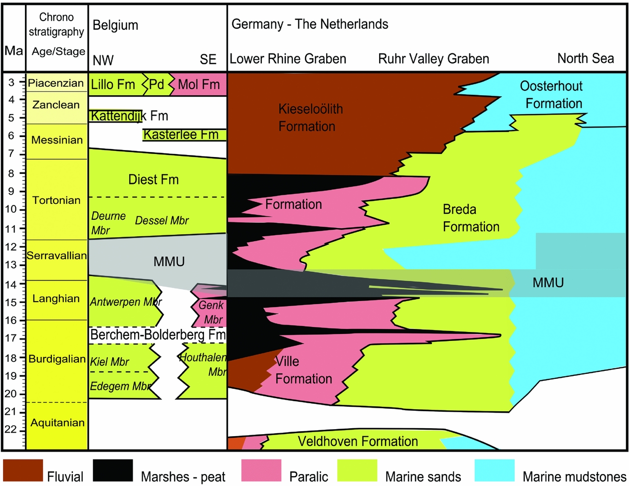
Figure 3. Miocene and Pliocene chronostratigraphy of the study area. The NW–SE section in Belgium runs approximately from Antwerp in the NW to the Limburg Campine – Ruhr Valley Graben (RVG) boundary in the SE. The section for Germany and the Netherlands is a SE–NW section through the Lower Rhine Embayment and RVG. Pd = Poederlee Formation. The approximate position of the Mid Miocene Unconformity (MMU) is also indicated. Modified from Van Adrichem Boogaert & Kouwe, Reference Van Adrichem Boogaert and Kouwe1997; Doornenbal & Stevenson, Reference Doornenbal and Stevenson2010; Adriaens, Reference Adriaens2015.
3.b. Previous heavy-mineral studies
Pioneering work on Neogene heavy minerals of the southern North Sea Basin as provenance indicators was done by Edelman & Doeglas (Reference Edelman and Doeglas1933). Their findings were confirmed and elaborated in many succeeding studies (Baak, Reference Baak1936; Tavernier, Reference Tavernier1943; Van Andel, Reference Van Andel1950; W. De Breuck, unpub. Ph.D. thesis, KU Leuven, 1959; Burger, Reference Burger1987). Edelman & Doeglas (Reference Edelman and Doeglas1933) defined two main provinces with a distinct heavy-mineral assemblage, the marine A province to the north and the continental B province to the south. Province A is characterized by garnet, hornblende and epidote, and becomes increasingly rich in this assemblage up to the Quaternary. This heavy-mineral assemblage can be found in the west and north of the Netherlands. An amphibole–epidote–garnet assemblage is typically related to collision orogen or orogenic root provenance terranes (Garzanti & Andò, Reference Garzanti, Andò, Mange and Wright2007). The orogenic source area for these deposits is inferred to be the Fennoscandian massif, as a similar heavy-mineral assemblage can be found on the Isle of Sylt, off the Danish coast (Edelman & Douglas, Reference Edelman and Doeglas1933; Olivarius et al. Reference Olivarius, Rasmussen, Siersma, Knudsen and Pedersen2011, Reference Olivarius, Rasmussen, Siersma, Knudsen, Kokfelt and Keulen2014). The Fennoscandian massif was drained by the large Baltic river system, which served as the major source of sediment to the North Sea Basin in the Late Miocene and Pliocene (Overeem et al. Reference Overeem, Weltje, Bishop-Kay and Kroonenberg2001). These sediments were then transported towards the southern North Sea Basin via shore-parallel currents. Another possible source area is the Scottish metamorphic belts (Gullentops & Huyghebaert, Reference Gullentops and Huyghebaert1999). Since the exact proportions of amphibole, epidote and garnet in such an assemblage are strongly controlled by hydraulic sorting effects, another independent provenance proxy such as zircon U/Pb dating should be consulted (Garzanti et al. Reference Garzanti, Andò, France-Lanord, Vezzoli, Censi, Galy and Najman2010), but such data are not available for these sediments. The continental B province of Edelman & Doeglas (Reference Edelman and Doeglas1933) is found in the east and southeast of the Netherlands and is defined by the near-absence of garnet and the absence of epidote and green hornblende and by a higher percentage (10–30 %) of parametamorphic minerals staurolite, kyanite and andalusite. It is linked with a continental source area to the south, through the RVG and local rivers, which drain the Palaeozoic Rhine–Ardennes Massif. Reworking of the Palaeogene sedimentary cover of the Rhine–Ardennes Massif and Brabant Massif could account for the high percentage of parametamorphic minerals (Parfenoff, Pomerol & Tourenq, Reference Parfenoff, Pomerol and Tourenq1970; Gullentops, Reference Gullentops1973; Gullentops & Huygebaert, Reference Gullentops and Huyghebaert1999). The Campine area of Belgium largely lies in the mixing zone between these two provinces.
The heavy-mineral associations identified in the Belgian Neogene are very similar to the ones defined by Edelman & Doeglas (Reference Edelman and Doeglas1933) (Tavernier, Reference Tavernier1943; W. De Breuck, unpub. Ph.D. thesis, KU Leuven, 1959). The Berchem Formation of the Lower to Middle Miocene in the western and central Campine Basin has an A association. The time-equivalent Bolderberg Formation in the eastern Campine Basin also has an A association in its marine lower Houthalen Member, while in the continental upper Genk Member the B association is recognized. The Tortonian Diest Formation has a more variable heavy-mineral assemblage, indicating mixing of A and B provinces. The B influence seems to increase to the east and south and from the bottom to the top of the Diest Formation. The Messinian Kasterlee Formation is also not consistent between different studies and appears to be quite similar to the Diest Formation. The Kieseloölite sand, which occurs in the far east of Belgium, of the latest Miocene and Pliocene has a typical B association.
3.c. Data collection and processing
For the Breda Formation, data were collected from the heavy-mineral database of the Dutch Geological Survey (TNO Utrecht). Heavy-mineral data from the Breda Formation are available for 156 samples from 16 different cores (Fig. 2). The depth of each sample is provided, the size fraction analysed is 63–500 µm, and the number of grains counted in these samples is around 200 (line counting). The heavy-mineral groups distinguished are tourmaline, garnet, Meuse-type garnet, epidote, hornblende, augite, staurolite, Al2SiO5 polymorphs (kyanite, andalusite, sillimanite) and a rest group.
Belgian Neogene heavy-mineral data were obtained from Gullentops & Huyghebaert (Reference Gullentops and Huyghebaert1999) and Geets & De Breuck (Reference Geets and De Breuck1991). In total, 626 heavy-mineral counts have been included, which are spread across the Belgian part of the study area. Up to 23 different heavy-mineral groups are listed, including tourmaline, zircon, rutile, garnet, epidote group minerals, many different amphiboles and pyroxenes, staurolite, the different metamorphic minerals and accessory minerals such as sphene and corundum. The data are ordered by formation and locality, but no indication of the depth of samples beneath the surface is given. A comparable dataset of Upper Eocene to Oligocene heavy-mineral data in the study area is also available, with similar format to the Belgian Neogene data and which includes 653 heavy-mineral counts (Geets, De Breuck & Jacobs, Reference Geets, De Breuck and Jacobs1985, Reference Geets, De Breuck and Jacobs1986). The number of transparent minerals counted in the Belgian datasets is 100 to 200 through line counting, and the fraction counted is 63–500 µm. Due to the analysis of a large grain-size range without coupled grain-size data, it is not possible to account for the relation between grain size and composition caused by hydraulic sorting effects, as done for example by Garzanti, Andò & Vezzoli (Reference Garzanti, Andò and Vezzoli2008, Reference Garzanti, Andò and Vezzoli2009). Indeed, variation in heavy-mineral composition related to sorting effects was traditionally regarded as noise (‘chance variations’) which cannot be reduced by counting a very large number of grains per sample. If no grain-size data are available, it is preferable to have data from a large number of samples (with a modest number of grains counted per sample), which permits ‘noise reduction’ by averaging (Edelman & Doeglas, Reference Edelman and Doeglas1933; Weltje, Reference Weltje2004). Deconvolution of compositional patterns into grain-size-related variations and provenance-related variations is not possible with these data, as no accompanying grain-size data are available.
Prior to data analysis, the datasets are rearranged to make them mutually compatible. The many mineral groups distinguished in the publications of the Belgian stratigraphy may be interesting for a detailed study of different samples, but to analyse the entire dataset simplification is preferable. Also, different authors may have identified certain minerals differently, such as the different amphiboles, and grouping these minerals together removes this problem. It must be noted, though, that harmonization of the datasets leads to a lower resolution for the final dataset compared to the original datasets, and some interesting details may be lost in the process. For all the data collected, the mineral groups which are retained are (1) tourmaline, (2) a rest group including zircon, rutile and accessory minerals, (3) staurolite, (4) the Al2SiO5 polymorphs (kyanite, andalusite and sillimanite), (5) garnet, (6) epidote group minerals (epidote, clinozoisite and zoisite) and (7) inosilicates (amphiboles and pyroxenes). The accessory minerals include sphene, corundum, dumortierite, scheelite, chloritoid and ‘saussurite’ (the latter is not a mineral species, but refers to turbid grains, possibly epidote–zoisite). Although amphiboles and pyroxenes can provide important separate provenance information, they are grouped together in the current analysis because pyroxenes occur only very rarely in all formations and regions of the study area and different pyroxenes are included in the results for the TNO data compared to the Belgian data. Finally, all zero values in the dataset are replaced by 0.1, as done by Von Eynatten, Barceló-Vidal, & Pawlowsky-Glahn (Reference von Eynatten, Barceló-vidal and Pawlowsky-Glahn2003). It is assumed that minerals with a 0% concentration occur only in trace amounts which are lower than the counting resolution. This must be done to include data which have zero values for certain minerals into the log-ratio analysis. This finished dataset is then analysed using the workflow described in Section 2. The datasets used for this study are available as an appendix in the online supplementary material at https://doi.org/10.1017/S0016756818000584
3.d. Results
3.d.1. Cluster analysis
The number of significant clusters in the Breda Formation is eight, based on a permutation test with confidence interval 99.9 % (Fig. 4). Three of these groups are made up of samples from the southern RVG, one group contains all samples of the northeastern RVG and some of the southern RVG, and the last four groups contain all samples of the Zeeland and Brabant area, just north of Belgium. The cluster analysis thus immediately indicates that the Breda Formation in these three different regions can be clearly distinguished based on the heavy-mineral content. It is also worth noting that the Zeeland and Brabant data are the furthest removed from the southern RVG data, with the northeastern RVG data in between. If the same analysis is done for the data of the Belgian Neogene, 26 significant clusters are formed. These data are more difficult to interpret as there is no clear grouping of regions or formations. The Berchem Formation of the lower Miocene is grouped quite well into three neighbouring clusters, which also contain many samples of the Diest Formation of the Antwerp Campine. Other formations, however, are too spread out to permit any conclusions. This result shows that cluster analysis is a good first exploratory tool, but if too many data are included without clear distinctions between groups, such as for the Belgian Neogene dataset, interpretation of the resulting clusters is not useful.

Figure 4. Cluster dendrogram resulting from a hierarchical cluster analysis of the CLR transformed heavy-mineral data of the Breda Formation (Dutch Miocene). The data are from three distinct regions, indicated in a different colour. The number of significant clusters is based on the permutation test of Clarke, Somer & Gorley (Reference Clarke, Somer and Gorley2008).
3.d.2. PCA
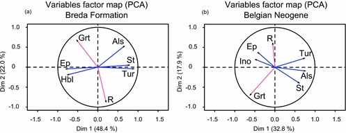
The two main principal components for the Breda Formation explain 70 % of the total variability of the dataset. The resulting plot of the loadings (Fig. 5a) indicates the correlation between the different heavy-mineral groups, with possible provenance significance. Epidote and hornblende are positively correlated with each other and negatively correlated with the Al2SiO5 polymorphs, staurolite and tourmaline. Approximately orthogonal, or independent of these minerals, garnet and the rest group are negatively correlated with each other. For the Belgian Miocene data, the two main components explain 51% of the total variability. The lower percentage compared to the Breda Formation dataset is expected because of the higher complexity of the data, also evidenced by the cluster analysis. Still, the pattern of the loadings is similar to the pattern observed for the Breda Formation (Fig. 5b).

Figure 5. Variables factor maps of a PCA of the CLR transformed heavy-mineral data. (a) Breda Formation (Dutch Miocene). (b) Belgian Neogene. Mineral abbreviations: Grt = Garnet, Als = Al2SiO5 polymorphs (andalusite, kyanite and sillimanite), St = Staurolite, Tur = Tourmaline, R = Rest group (zircon, rutile and accessory minerals), Hbl = Hornblende, Ep = Epidote, Ino = Inosilicates (amphiboles and pyroxenes). Minerals with the same colour are approximately parallel or opposite. Minerals with a different colour are approximately orthogonal.
3.d.3. Log-ratio plots
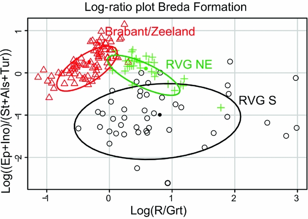
The four mineral groups which have been recognized by PCA are used to make log-ratio plots which capture the maximum amount of information. A first log-ratio (LR1) of epidote and inosilicates vs Al2SiO5 polymorphs, staurolite and tourmaline is plotted against a second approximately independent log-ratio (LR2) of rest group minerals vs garnet.
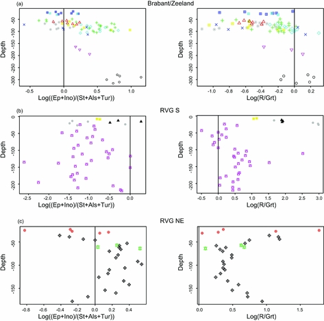
The plot of the Breda Formation shows a complete separation between the Brabant data and the southern RVG data with the northeastern RVG data in between (Fig. 6), as expected based on the cluster analysis. The values of LR1 are similar or slightly higher in the Brabant area compared to the northeastern RVG, but markedly higher compared to the southern RVG. The values of LR2 are higher in both RVG areas. Some samples of the southern RVG have a much higher LR2 value due to the lack of garnet in those samples. When plotting LR1 vs depth for the Brabant area a very slight decrease in LR1 can be observed towards the surface (Fig. 7a). However, this decrease is mainly observed between different cores, in which the Breda Formation is present at different depths. Due to the lack of age information linked to the samples, no statements can be made on the variation in LR1 through the Miocene because the decrease could both be caused by regional variations within the basin or due to secondary effects. A plot of LR2 vs depth does not indicate a trend. In the southern RVG, no trend can be observed for LR1 or LR2 vs depth (Fig. 7b). In the northeastern RVG, however, a trend in both LR1 and LR2 seems to be present (Fig. 7c). LR1 increases from the bottom up to a depth of about 100 m and then decreases again. The opposite is true for LR2.


Figure 7. Plots of LR1 and LR2 vs depth for the three different regions analysed for the Breda Formation (Dutch Miocene). Data points of a different colour/symbol belong to different cores. (a) Brabant/Zeeland. (b) Southern RVG. (c) Northeastern RVG. Mineral abbreviations: see Figure 5.
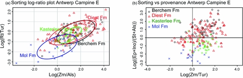
The Belgian Neogene data show a large spread on the log-ratio plot. A regional subdivision of the data again shows a NW–SE variation, with the Antwerp area having the highest LR1 values (Fig. 8a). Very high LR2 values in the Limburg Campine area, the Hageland area and the Flemish Hills are again caused by a lack of garnet. There is a large overlap between the regional groups as many different formations are included in each regional group. In order to study regional variations within a single time interval, a regional subdivision of the Upper Miocene Diest Formation has been made, which covers most of the study area (Fig. 8b). LR1 is slightly higher in the Antwerp area and slightly lower in the Flemish Hills compared to the other areas. LR2 is higher towards the south and east where the Formation is less deeply buried. Samples of the Limburg Campine area, Hageland Hills and almost all samples of the Flemish Hills have very high values for LR2. These are all samples from outcrops or shallow subcrops. To capture the temporal evolution within one region, the different formations which occur in the Antwerp Campine area are plotted for both the area west of Kasterlee and east of Kasterlee (Fig. 8c, d). From Lower Miocene to Pliocene there is a marked decrease in LR1 and an increase in LR2 for the eastern part of the Antwerp Campine area. In the western Antwerp Campine area, no significant trend can be observed. There is no consistent trend of LR1 vs LR2 within each formation. The values of the Berchem Formation are the most similar to the values of the Breda Formation in the Brabant/Zeeland area whereas the eastern Kasterlee Formation and the Mol Formation are most similar to the southern RVG. A similar analysis of the Limburg Campine area does not yield significant results as all formations overlap. Overall the values of LR1 are lower in the Limburg Campine compared with the Antwerp Campine (Fig. 8a).
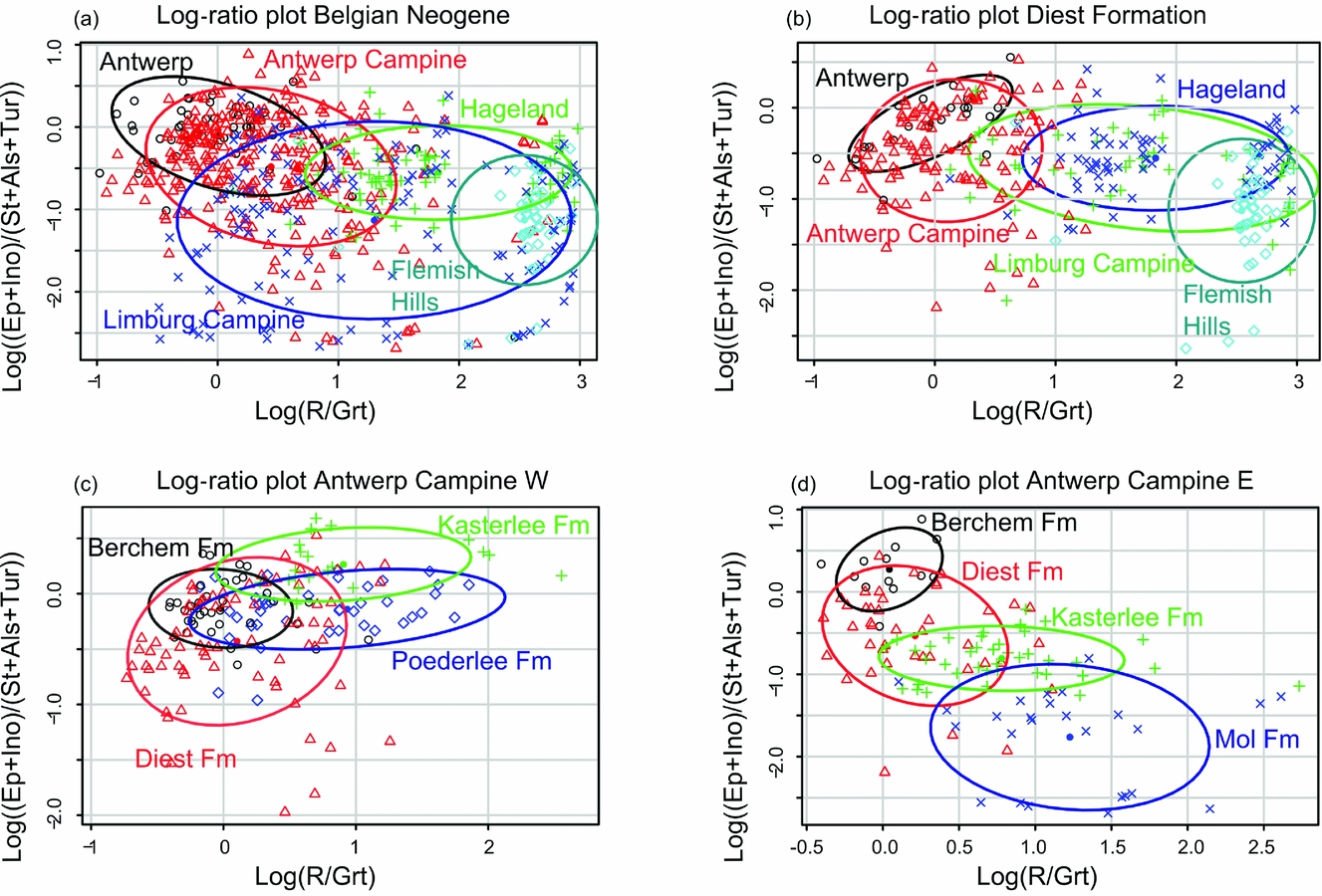
Figure 8. Log-ratio plots of the Belgian Neogene heavy-mineral data. (a) Log-ratio plot of the heavy-mineral data of the Belgian Neogene separated by region. (b) Log-ratio plot for the Tortonian Diest Formation separated by region. (c) Log-ratio plot of the western Antwerp Campine basin separated by formation. (d) Log-ratio plot of the eastern Antwerp Campine basin separated by formation. 2σ confidence ellipses are added for visualization. Mineral abbreviations: see Figure 5.
3.d.4. Checks and balances
3.d.4.a. Sorting
Since the original Belgian data are separated into more individual heavy-mineral species instead of larger heavy-mineral groups, different log-ratios can be made which can indicate sorting. Minerals within the previously defined groups, such as epidote and inosilicates, are not expected to have a significant difference in grain size as they have similar densities and thus cannot be used to indicate a sorting effect. Alternatively, a log-ratio of zircon vs Al2SiO5 polymorphs is plotted against a log-ratio of rutile vs tourmaline (Fig. 9a). Both zircon and rutile are very high-density minerals and typically occur in the finer size fraction of each sample, as an effect of the settling-equivalence principle (Rubey, Reference Rubey1933). Tourmaline and Al2SiO5, in contrast, typically occur in the coarser size fraction of each sample. Such a plot does show a trend for the Antwerp Campine area, based on the shape of the ellipses in Figure 9a. The data points of the different formations of the Miocene, however, completely overlap, indicating that grain-size differences among formations are not a significant control on variations in heavy-mineral content. Only the data of the Pliocene Mol Formation plot at lower values, which could mean that a coarser grain size is partly responsible for the low LR1 values of this formation.

Figure 9. Log-ratio plots based on the available heavy-mineral data, which can be used as a proxy for the effects of sorting on variations in the heavy-mineral composition. (a) Plot of two sorting log-ratios, with higher values for both as a proxy for a decrease in grain size. (b) A similar sorting log-ratio vs a provenance log-ratio (LR1). Grt = Garnet, Als = Al2SiO5 polymorphs (andalusite, kyanite and sillimanite), St = Staurolite, Tur = Tourmaline, Zrn = zircon, Rt = rutile, Ep = Epidote, Ino = Inosilicates (amphiboles and pyroxenes).
When plotting a provenance log-ratio, epidote and amphibole vs Al2SiO5 polymorphs and staurolite, against a sorting log-ratio, zircon vs tourmaline, no convincing trend can be observed (Fig. 9b). Differences along the provenance log-ratio are much more apparent than along the sorting log-ratio.
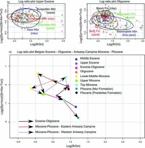
The Upper Eocene and Oligocene data can be used to demonstrate the final proxy, as heavy-mineral data of both sandy and clayey units are present. On the log-ratio plot, no distinction can be made between the sandy and clayey sediments, indicating that grain size is not a dominant control on the heavy-mineral composition of these units, under the assumption that the provenance of these different units is similar (Fig. 10a).

Figure 10. Log-ratio plots of the Belgian Palaeogene data, for assessment of sorting effects and recycling. (a) Log-ratio plots of different sandy and clayey units for the Upper Eocene and Oligocene of northern Belgium. (b) Log-ratio plot indicating the average values of different stratigraphic groups from the Middle Eocene to the Pliocene. Mineral abbreviations: see Figure 5.
3.d.4.b. Weathering and recycling
LR2 is the log-ratio of ultrastable minerals vs garnet. Garnet is unstable under acidic conditions or at deep burial depths (Morton & Hallsworth, Reference Morton and Hallsworth1994, Reference Morton and Hallsworth1999; Milliken, Reference Milliken, Mange and Wright2007; Van Loon & Mange, Reference Van Loon, Mange, Mange and Wright2007). The maximum burial depth of the samples in this study is 300 m in the Brabant/Zeeland area. The burial depth of the samples in the Belgian part of the study area ranges from outcrops to 200 m and this is not known to have been much deeper in the past. Due to the limited burial of the Miocene sediments in the study area, burial diagenesis is not an important factor to take into consideration (Morton & Hallsworth, Reference Morton, Hallsworth, Mange and Wright2007). Acidic conditions may occur in the shallow subsurface due to the circulation of meteoric fluids or in the deeper subsurface, for example due to leaching beneath a lignite layer. The contrasting resistance to chemical weathering between garnet and the ultrastable minerals under these conditions implies that LR2 can be used as a weathering indicator.
By plotting LR1 and LR2 vs depth for the Breda Formation, the effect of recent superficial weathering can be observed. The depth vs LR1 plots for the Brabant area and southern RVG do not show a trend as discussed in Section 3.4.3. The same is true for LR2 vs depth, which is a good indication of the lack of weathering as an important controlling factor. A few samples belonging to shallow cores in the southern RVG do have high LR2 values, indicating these samples may be more heavily weathered (Fig. 7b). The patterns observed for LR1 and LR2 vs depth in the northeastern RVG (Fig. 7c) could indicate that weathering does affect both ratios, though the increase in LR2 and decrease in LR1 start already at a depth of 100 m. Weathering at the time of deposition or due to later leaching, for example beneath a lignite bed, can only be tested if sufficiently detailed stratigraphic information is present as well.
For the eastern Antwerp Campine area, an overall correlation seems to be present between LR1 and LR2. Younger Formations have both a lower value of LR1 and a higher value of LR2. As LR2 can indicate weathering, this could indicate a weathering dependence of LR1 as well. However, if weathering were the dominant factor of the variation in LR1, the same correlation between LR1 and LR2 should also be observed within each defined group. As seen in Figure 8d, the value of LR1 does not decrease with an increasing value of LR2 within each defined formation. Samples from outcrops of the Flemish Hills and the Hageland Hills which are strongly weathered do have a very high LR2 value, as garnet is no longer present (Fig. 8b). For the Hageland Hills, both samples with no garnet – very high LR2 – and samples with a few percent of garnet – lower LR2 – are present, yet their value for LR1 is approximately the same. LR1 is thus not equally affected by weathering.
The possibility of recycling can be assessed by a comparison with stratigraphically older intervals. The Palaeogene data are separated into formations belonging to the Middle Eocene, Upper Eocene, Eocene–Oligocene boundary and Oligocene. There is a large spread and overlap of the groups based on LR2, but a trend can again be recognized in LR1. LR1 increases from the Middle Eocene to Oligocene (Fig. 10b). Similar values of LR1 occur in the Lower Miocene compared to the Oligocene, followed by a decrease in LR1 up to the Pliocene for the eastern Antwerp Campine area and an erratic pattern in the western Antwerp Campine area. For LR2, there is an erratic decrease up to the Lower Miocene, followed by an increase up to the Pliocene. The observed pattern may indicate a cyclic provenance variation and/or the similarity between the Palaeogene and Neogene heavy-mineral data could indicate that significant reworking has taken place.
3.d.5. Spatial interpolation
As discussed above, neither LR1 (epidote and inosilicates vs Al2SiO5 polymorphs, staurolite and tourmaline) nor LR2 (rest group minerals vs garnet) is strongly affected by grain size and only LR2 is significantly affected by weathering. LR1 is considered to be mainly influenced by provenance variations and can be used as a provenance proxy for spatial interpolation. In the Dutch part of the study area, most of the Miocene is grouped into one formation, the Breda Formation. As such, no time slices can be distinguished and a spatial interpolation by time slice is not possible. In the Belgian part of the study area, four relevant time slices can be distinguished: (1) the Burdigalian to Langhian, represented by data of the Berchem Formation in the west and the lower member of the Bolderberg Formation in the east, (2) the Tortonian, represented by data of the Diest Formation, (3) the Messinian, represented by data of the Kasterlee Formation, and (4) the Pliocene, represented by data of the Poederlee Formation in the west and Mol Formation in the east. The average LR1 values for each time slice by location are interpolated using a kriging algorithm. The resulting spatial interpolation for each time slice is split into three discrete zones in order to avoid unnecessary detail (Fig. 11a).
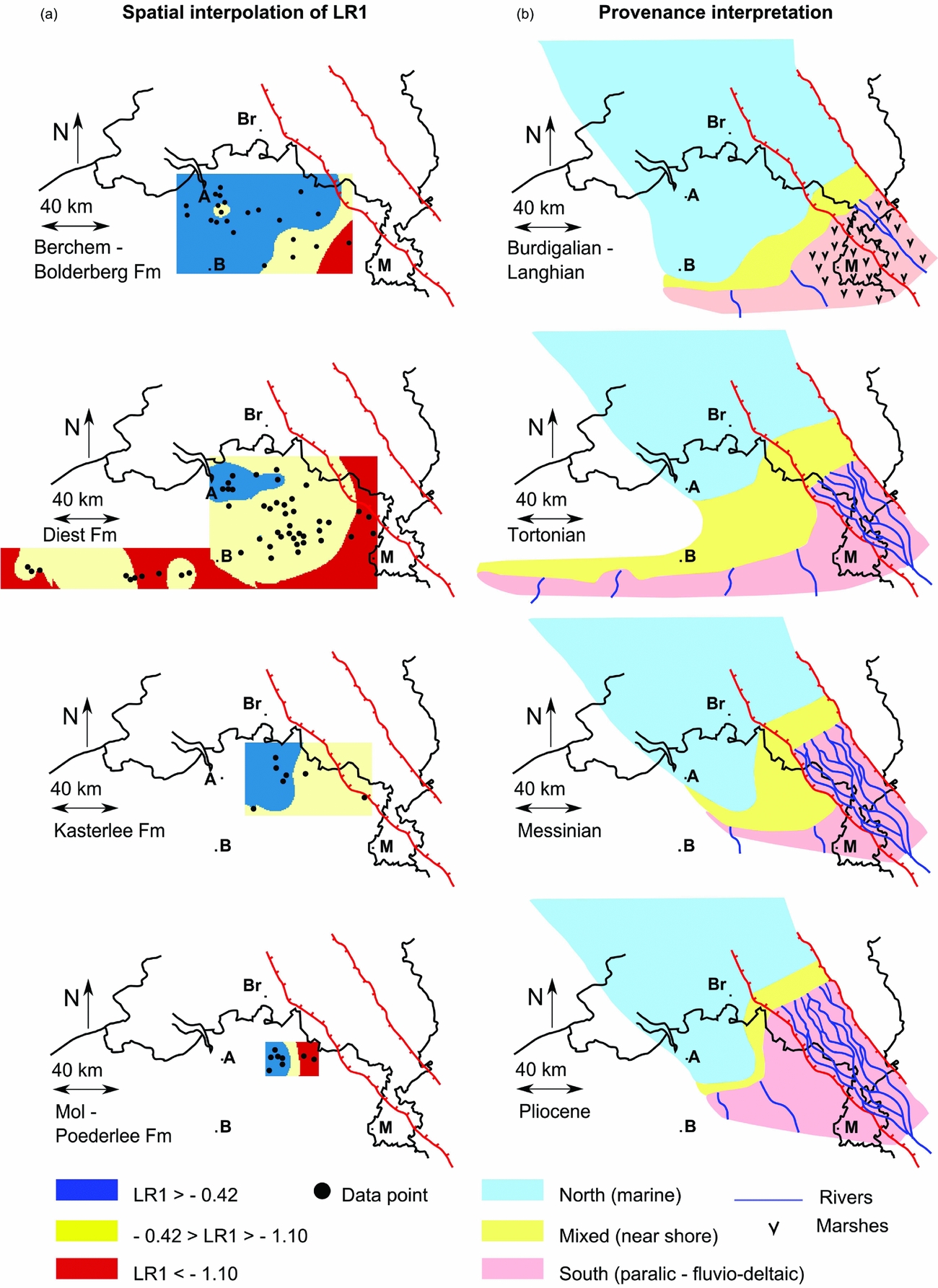
Figure 11. Geospatial interpolation and interpretation. (a) Spatial interpolation of the average LR1 values (LR1 = Log(Epidote + Inosilicate)/(Staurolite + Al2SiO5 + Tourmaline)) by location for each time slice. For each time slice, locations at which data are available are indicated. (b) Provenance interpretation based on the geospatial interpolation. A = Antwerp, B = Brussels, Br = Breda, M = Maastricht.
3.e. Provenance implications
In the Brabant/Zeeland area, the Breda Formation is characterized by high LR1 values, in contrast to the southern RVG area, where low LR1 values are recorded (Fig. 6). There is no apparent variation in LR1 throughout the Breda Formation within these regions. Epidote and amphibole can thus be linked to a northern source area and the metamorphic minerals and tourmaline to a southern source area. This coincides with the typical A and B province defined by Edelman & Doeglas (Reference Edelman and Doeglas1933). Garnet is also related to the A province in the classic scheme. As garnet is strongly affected by chemical weathering compared to zircon and titanium minerals, however, LR2 is not used for provenance interpretations in this study. In the northeastern RVG, a variation with depth can be observed with an increase in LR1 followed by a decrease towards the top (Fig. 7c). This could indicate that sediment is increasingly supplied to this area from the northern source during most of the Miocene, but that a strong increase in input from the Rhine occurs during the latter part of the Miocene. This could coincide with the long transgressive–regressive cycle proposed by Schäfer et al. (Reference Schäfer, Utescher, Klett and Valdivia-Manchego2005), yet this interpretation cannot be confirmed due to a lack of biostratigraphic data coupled to this observation.
In contrast to the fairly constant provenance in the Dutch Brabant area and the southern RVG, significant variations can be observed in the Campine Basin. As expected, sediments which occur more to the northwest are affected more by the northern source and sediments which occur more to the southeast are affected more by the southern source (Fig. 11). More importantly, a change in provenance of the sediments occurs from the Early Miocene to Pliocene (Fig. 11b). In the eastern Antwerp Campine area, there is a gradual increase in input from the southern source area throughout the Neogene, as each younger formation has a slightly lower value for LR1 (Fig. 8d). The top Miocene Kasterlee Formation already has LR1 values similar to the southern RVG. For the Pliocene Mol Formation it can be stated that the pre-Rhine was the dominant source of sediments in the area. Coeval to the Kasterlee and Mol Formations the coarse fluvio-deltaic quartz sand of the Kieseloölite Formation was deposited in the RVG on top of the marine glauconite sands of the Breda Formation (Van Adrichem Boogaert & Kouwe, Reference Van Adrichem Boogaert and Kouwe1997) which is linked to a further northwestern extent of Rhine influence during this period (Fig. 11b). More to the west of the Campine Basin, no change in provenance can be implied based on the data (Fig. 8c). The northern source remains the dominant source of sediment for the western Campine Basin up to the Pliocene, similar to the Dutch Brabant area. This palaeogeographic interpretation is confirmed by the spatial interpolation of provenance proxy LR1, which convincingly illustrates a gradual shift towards the northwest of the influence of southern sediments, throughout the Neogene (Fig. 11b).
The suggestion by Houthuys (Reference Houthuys2014) that the Flemish Hills sand is not related to the Hageland Diest sand cannot be confirmed by the heavy-mineral analysis. The heavy-mineral data indicate at least a similar provenance for the Flemish Hills sand and the Hageland sand (Fig. 8b), though a determination of their stratigraphic position cannot be made based on these data. The Flemish Hills sand has a very high value for LR2 as it is strongly weathered. It also has only a slightly lower value of LR1 compared to the Hageland Hills, which can be expected as it is further removed from the northern source area and the strong weathering may have also slightly lowered the LR1 value due to weathering of epidote and inosilicates (Fig. 8b). Reworking of Palaeogene and older Miocene deposits into younger Miocene successions constitutes an important contribution to the total sediment supply as noted by various observations, such as the dating of reworked glauconite and fossils (De Meuter & Laga, Reference De Meuter and Laga1976; Vandenberghe et al. Reference Vandenberghe, Laga, Steurbaut, Hardenbol, Vail, Graciansky, Hardenbol, Jacquin and Vail1998, Reference Vandenberghe, Harris, Wampler, Houthuys, Louwye, Adriaens, Vos, Lanckacker, Matthijs, Deckers, Verhaegen, Laga, Westerhoff and Munsterman2014; Verhaegen et al. Reference Verhaegen, Adriaens, Louwye, Vandenberghe and Vos2014). The similar heavy-mineral composition of the Eo–Oligocene sediments compared to the Neogene sediments also indicates that substantial reworking is possible, but the amount of reworking cannot be estimated based on the data available. Jacobs (Reference Jacobs1995) proposes a dominant southern sediment input for the Eocene sediments, whereas a more open marine environment with northern sediment supply via longshore currents is proposed for the Oligocene units of the area (Vandenberghe & Mertens, Reference Vandenberghe and Mertens2013), which also fits with the patterns in Figure 10b. As reworking of Palaeogene sediments is mainly caused by rivers at the southern edge of the basin, the signature of reworking is in particular present in the southern source composition and as such does not significantly alter the interpretation of varying provenance throughout the Neogene.
To summarize, the LR1 values of the Brabant/Zeeland area and southern RVG can be interpreted as representative for the northern source and the southern source respectively. The Campine Basin is a zone of mixing. Already during the Miocene, this area was significantly affected by the southern input, in contrast to areas more to the north where the southern continental input only became important from the late Pliocene onwards (Cameron, Bulat, & Mesdag, Reference Cameron, Bulat and Mesdag1993; Gibbard & Lewin, Reference Gibbard and Lewin2016).
4. Discussion and conclusion
There are no strong contrasts between the results discussed here and available knowledge in the literature, going as far back as Edelman & Doeglas (Reference Edelman and Doeglas1933), which indicates that the results based on the multivariate statistical approach are valid. However, the proposed statistical workflow does have strong advantages compared with the classic approach of visually analysing large data tables or plotting the data in cumulative heavy-mineral diagrams. Via log-ratio transformation of the data, they can be analysed with multivariate statistics. The log-ratio plots presented here provide quick data visualization and a more objective way of identifying different groups in the data and interpreting the observed differences. Furthermore, multiple distinguished types of groups can be quickly analysed, for example based on stratigraphy or region. The multivariate statistical workflow also enables users to calculate probability regions and add a more quantitative and predictive aspect to the final results. Finally, this workflow offers the possibility of extracting one single proxy of provenance from a large multivariate dataset, which can be used for geospatial interpolation, further aiding palaeogeography and provenance interpretations. Using this workflow, open questions in stratigraphy and provenance can be examined in further detail with existing or new data. Of course, such a statistical workflow only works properly if the input data are of decent quality and if the operator has a good knowledge of the geological situation of the samples. The proposed methodology serves to gain as much information as possible from big datasets, but it cannot provide information which is inherently not captured in the data. For instance, no bulk-sediment data are available for the legacy data analysed in this study, and therefore it is not possible to establish a direct link between bulk mass transfer and heavy-mineral analyses (Weltje & Von Eynatten, Reference Weltje and von Eynatten2004; Garzanti, Reference Garzanti2016).
Although this study demonstrates that a lot of information can be efficiently extracted from such legacy datasets, the results would benefit from the addition of other data types. The effects of hydraulic sorting on the heavy-mineral composition can potentially be eliminated or minimized by adding grain-size data (cf. Bloemsma et al. Reference Bloemsma, Zabel, Stuut, Tjallingii, Collins and Weltje2012) or by using a two-way classification of the point-counting data, which includes both the heavy-mineral species and the grain size or grain-size range. Biostratigraphic data directly coupled to the heavy-mineral data improve temporal constraints, and seismic and log data would help to correlate the different boreholes. In such a comprehensive approach, including the application of data analysis techniques demonstrated in this study, heavy-mineral data could be used in an integrated mass-balance approach to sedimentary provenance analysis.
Acknowledgements
We would like to thank Professor Emeritus Noël Vandenberghe (KU Leuven) for sharing his valuable comments on the text. This research is funded by FWO (Flanders Research Foundation) grant 1105818N. We thank reviewers Alberto Resentini and Eduardo Garzanti for their valuable comments and suggestions.
Declaration of interest
None.
Supplementary material
To view supplementary material for this article, please visit https://doi.org/10.1017/S0016756818000584