I. Introduction and Research Question
Changing climate, global warming, and weather fluctuations have a special importance for agricultural production. The relationship between weather and wine production is especially strong; therefore, fine wine has characteristics that make this connection an interesting topic for economic analysis (Ashenfelter and Storchmann, Reference Ashenfelter and Storchmann2016). As German wine regionsFootnote 1 are situated near the northern boundary of commercial grape growing, stretching from the south (47.32°N) to the north (51.32°N) of Germany, wine producers depend highly on favorable weather conditions (Ashenfelter and Storchmann, Reference Ashenfelter and Storchmann2010).
German wines are categorized by the degree of ripeness of the grapes, measured as the content of natural sugar in the must (grape juice) upon harvest; the German term is degree Oechsle.Footnote 2 The higher the sugar level, the higher the wine will be categorized. The quality categories and responding Oechsle thresholds vary from region to region. For instance, in the region Pfalz (Palatinate), the quality levels fall into the following brackets: Qualitätswein (Qba) (60–72° Oechsle), Kabinett (73–84° Oechsle), Spätlese (85–91° Oechsle), Auslese (92–119° Oechsle), Beerenauslese and Eiswein (120–149° Oechsle), and Trockenbeerenauslese (>150° Oechsle). With the exception of Qualitätswein (Qba),Footnote 3 it is illegal to add sugar to the must (Ashenfelter and Storchmann, Reference Ashenfelter and Storchmann2010).
This paper examines to what extent weather and annual weather fluctuations affect the total wine production and the shares of different quality categories in Germany.
II. Previous Literature
A growing number of studies has examined the potential impact of weather variation and, as their long-run expression, climatic changes on wine quality, grape yields, and production levels. Ashenfelter and Storchmann (Reference Ashenfelter and Storchmann2016) provide a literature review of one wine and climate change. Measures of quality can be divided into direct and indirect measures. Direct measures rely on quantifiable wine characteristics, such as alcohol level or the sugar content of the must (degree Oechsle), while indirect measures refer to vintage scores, quality ratings from wine guides, expert ratings, or prices for rankings.
The research dealing with direct measures of quality shows contradictory results. Ashenfelter (Reference Ashenfelter2008) stresses that the quality of any fruit depends on weather during the growing season and that some regions have more- and less-pronounced weather fluctuations. High-quality vintages for Bordeaux wines, for example, correspond to years with a dry August and September, a warm growing season, and a wet previous winter. Storchmann (Reference Storchmann2005) suggests, in an analysis of the impact of weather on wine quality of Schloss Johannisberg for the years 1700 to 2003, that warming improves the quality of wine. Alston et al. (Reference Alston, Fuller, Lapsley and Soleas2011) find, for the years 1980–2005, that rising temperatures contribute to higher sugar levels of wine grapes in California, as Brix levels increased by an average of 0.23 percent annually. Alston et al. (Reference Alston, Fuller, Lapsley and Soleas2011, Reference Alston, Fuller, Lapsley, Soleas and Tumber2015) find that alcohol levels have increased in U.S. and Canadian wineries due to higher Brix levels. Mira de Orduña (Reference Mira de Orduña2010) finds that higher growing-season temperatures cause sweeter musts and stronger wines, but that extremely high temperatures may negatively affect wine aroma and color. Leeuwen and Darriet (Reference Leeuwen and Darriet2016) show that higher temperatures lead to higher quality levels in Languedoc during the years 1984 to 2013, but this tendency could change due to water deficits. Oczkowski (Reference Oczkowski2016) identifies winners and losers of temperature changes, depending on the grape variety. This paper adds to this body of research by focusing on all thirteen German wine regions. I use the output (in hectoliters) of wine of different quality categories as a direct measure of quality, as these categories are directly related to the sugar content of the must.
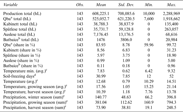
Most of the above-mentioned literature applies hedonic approaches. These approaches all relate dependent variables to their visible characteristics or attributes, which are continuously measurable (quantitatively) or not (qualitatively) (Oczkowski, Reference Oczkowski1994). Authors often choose the average temperature and the total rainfall over the growing and winter season as weather variables (Ashenfelter and Storchmann, Reference Ashenfelter and Storchmann2010), but this paper applies a hedonic approach using various average temperatures (during the whole,Footnote 4 growing, and harvest seasons), the number of soil-freezing days during the growing and harvest seasons, and the total precipitation during the winter, growing, and harvest seasons (see Table 1).
Table 1 Descriptive Statistics

a Qba: Qualitätswein. b Batbaice: Beerenauslese/Trockenbeerenauslese/Eiswein. c Temperature and temperature min.: avg. of the whole season (winter, growing, harvest). 4 Soil-freezing days: sum of days with soil temperatures < 0 degrees during the growing and harvest seasons. 5 Winter season: Dec. 1 to Feb 28; Growing season: Mar. 1 to Sep 15; Harvest season: Sep. 16 to Oct. 31.
III. Data on Weather and Quality
Because meso-weather data for the vineyard in which the grapes were grown are almost never available, most studies rely on weather data from nearby weather stations. This study draws on data from regional weather stations that are located within each of the thirteen German viticultural regions and cover the time period from 2003 to 2013.Footnote 5
Lecocq and Visser (Reference Lecocq and Visser2006) for Bordeaux and Haeger and Storchmann (Reference Haeger and Storchmann2006) for California, respectively, show that within a homogenous wine region, local weather data yield little additional explanatory power over regionally aggregated weather data; but this paper refers to data from regional weather stations, as weather conditions in Germany differ significantly between regions. The German Wine Institute (2003–2016) provides data on the output of hectoliters per quality category and the share of output for Qualitätswein (Qba), the lowest-quality category; Kabinett; Spätlese; and Auslese. For Beerenauslese (BA), Trockenbeerenauslese (TBA), and Eiswein (ICE), which are deemed the highest quality, only aggregated figures exist, here denoted as BA-TAB-ICE or “Batbaice.” Descriptive statistics for the data are presented in Table 1.
IV. Methods and Results
Suppose there are two wines, one of high quality (H) and another of low quality (L). The quantity produced in each segment, i.e., QH and QL, depends on weather (W) in two ways. First, beneficial weather, depicted by a high W value, has a positive impact on the yields of both wines. Second, T will also affect the likelihood of each wine's falling into the L or H bracket. That is, although conducive W conditions may directly boost the yield of H wine produced even at constant L and H shares, they also increase the likelihood of any given wine's falling into the H bracket. The overall effect in H wines is unambiguous, because both effects increase their quantity produced.
Therefore,
The marginal effect of T on QH is then
Likewise, QL equals
Yield-wise, W is assumed to have positive marginal effect for both wines, i.e.,
Share-wise, however, the effects are different:
That is, the overall effect of beneficial weather on the quantity of lower-quality wine produced is supposed to be ambiguous.
Empirically, I estimate the impact of weather first on total production and then on production shares in each of the five quality categories by applying a standard panel data model with the thirteen wine regions for the time period of 2003 to 2013.
I estimate equation (1) with the logarithm of the total production as dependent variable y, regional fixed effects, and cluster robust standard errors:
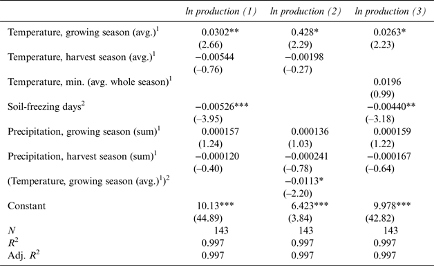
where w it is a k*1 vector of weather variables and β is a k*1 vector of parameters to be estimated. The error term u it consists of a time-invariant individual-specific unobserved effect αi and the idiosyncratic error term νit (e.g., Hoyos and Sarafidis, Reference Hoyos and Sarafidis2006). Table 2 shows the results.
Table 2 Regional Fixed-Effects Estimation on Total Production

Robust t statistics are in parentheses; significance levels are *p < 0.05, **p < 0.01, and ***p < 0.001. 1 Winter season: Dec. 1 to Feb. 28; growing season: Mar. 1 to Sep. 15; harvest season: Sep. 16 to Oct. 31. 2 Soil-freezing days: sum of days with soil temperatures < 0 degrees during the growing and harvest seasons.
The results suggest a significantly positive impact of average growing-season temperatures on production, whereas additional soil-freezing days appear to exert a negative effect.
When analyzing the impact of weather on the share of production, the following problem arises due to the categories’ interdependent dependence: an increase in the share of one category implies a decrease somewhere else. As a result, the error terms are correlated across equations. In this case, it seems appropriate to employ Zellner's (Reference Zellner1962) Seemingly Unrelated Regression (SUR), which allows for jointly estimating a system of equations with exogenous predictors. Zellner bases his approach on constructing a stepwise algorithm using first the Generalized Least Squares (GLS) approach for the estimation of each individual-specific equation and then using the Maximum Likelihood approach for estimating the residual covariance matrix (Sarafidis and Wansbeek, Reference Sarafidis and Wansbeek2012). Table 3 reports the results of the SUR approach.
Table 3 Results of the SUR Model for Shares of Production

t statistics are in parentheses; significance levels are *p < 0.05, **p < 0.01, and ***p < 0.00. a Winter season: Dec. 1 to Feb. 28; growing season: Mar. 1 to Sep. 15; harvest season: Sep. 16 to Oct. 31. b Qualitätswein (Qba). c Batbaice: Beerenauslese/Trockenbeerenauslese/Eiswein.
As expected, temperature's positive impact on the respective shares increases with increasing quality level. That is, the warmer the growing season, the more likely a certain wine will be classified in a superior quality bracket. In contrast, rainfall appears to have no consistent and significant effect on the quality share distribution. This may be due to the local character of precipitation, i.e., the weather station some 20 km away from the vineyard may record some rain while the vineyard has been dry, and vice versa.
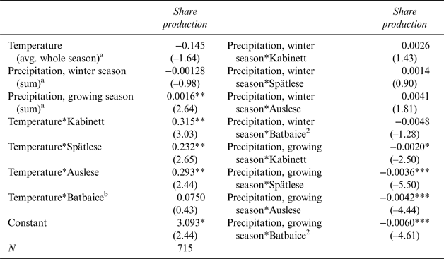
The SUR model may not be the perfect way to approach a regression where the explained variables vary within a 0–1 boundary, as SUR may predict share values that are outside this range. I, therefore, also used a generalized linear model (GLM) that allows predicted values to only fall within the 0–1 boundary. The result is the same as for equation (1), but now with the share of production as a dependent variable (UCLA, 2017). I also added various additional interaction terms as independent variables; Qualitätswein (Qba) is the reference category. Table 4 shows the results of this estimation.
Table 4 Results of the GLM Approach for Shares of Production

Robust t statistics are in parentheses; significance levels are *p < 0.05, **p < 0.01, and ***p < 0.00. a Winter season: Dec. 1 to Feb. 28; growing season: Mar. 1 to Sep. 15; harvest season: Sep. 16 to Oct. 31. b Batbaice: Beerenauslese-Trockenbeerenauslese-Eiswein.
Similar to the SUR results, the GLM panel results suggest an increasingly positive impact of temperature with higher qualities. However, the temperature effects on the highest category, Batbaice (Beerensauslese-Trockenbeerenauslese-Eiswein), are not significantly different from those on the lowest category, Qualitätswein (Qba). This result may be surprising at first, but one may consider the fact that the aggregation Batbaice includes Eiswein, a wine category that does not benefit from a warm growing season. Eiswein is made from frozen grapes, and German wine law stipulates that the congelation of at least–7°C must take place on the vine, which is not attained every year. This makes the production of Eiswein risky, and only inferior vineyards are devoted to it.
The GLM results also suggest an increasingly deteriorating effect of the growing season's precipitation on the quality shares, especially within higher-quality brackets (Table 4).
Overall, the results of the SUR and the GLM approaches convey a significantly positive impact of average temperatures and average minimum temperatures during the whole season on the output shares of wine in higher-quality categories, while precipitation during the growing season reduces this share significantly.
V. Conclusion
The analysis suggests that the hypothesis that beneficial weather—here indicated by rising average temperatures during the growing season—will increase total wine production holds true, while additional soil-freezing days seem to have an adverse effect on total wine production. Regarding the shares of wine in higher-quality categories, rising average and rising minimum temperatures have a significantly positive impact on wine in higher-quality brackets.
The European Environmental Agency (2016) projects annual average land temperature over Europe to increase over the rest of this century by around 2.4 °C to 4.1 °C; this predicted rise in temperatures may lead to higher total outputs and higher shares of outputs of wines in higher-quality categories in Germany. Expected drier growing seasons (Lübbecke, Reference Lübbecke2010) as well as the decrease in the number of growing-season freezing days may add to this effect.


