


1. Introduction
Solitary trees are very efficient in reducing the mean wind speed. Experimental observations of this capability have been performed by both wind tunnel studies on young trees (Lee, Lee & Lee Reference Lee, Lee and Lee2014; Manickathan et al. Reference Manickathan, Defraeye, Allegrini, Derome and Carmeliet2018) and tree-shaped structures (Gromke & Ruck Reference Gromke and Ruck2008; Bai, Meneveau & Katz Reference Bai, Meneveau and Katz2012; Chan et al. Reference Chan2020), as well as in full-scale experimental studies (Dellwik et al. Reference Dellwik, van der Laan, Angelou, Mann and Sogachev2019). Due to this characteristic, trees act as obstacles to the wind in the surface layer of the atmospheric boundary layer. Their presence over an area leads to an increase of the amount of momentum that the surface absorbs (Raupach Reference Raupach1992). Parameterising this effect accurately (Hopwood Reference Hopwood1996) could improve the accuracy of weather modelling (Hasager et al. Reference Hasager, Nielsen, Jensen, Bøgh, Christensen, Dellwik and Søgaard2003) as well as improve the estimated impact of trees in shelter-belt applications (Miller, Rosenberg & Bagley Reference Miller, Rosenberg and Bagley1974).
The loss of momentum is the result of the drag that the tree is exerting on the flow. In the case of bluff bodies the drag has traditionally been expressed by a force vector  $\boldsymbol {F}_d$ using a non-dimensional drag coefficient
  $C_d$
$C_d$
 \begin{equation} \boldsymbol{F}_d=\tfrac{1}{2}\rho C_d A |\boldsymbol{u}| \boldsymbol{u}, \end{equation}
where  $\rho$ is the air density,
  $A$ the frontal area of a body and
  $\boldsymbol {u}$ is the wind speed vector. Trees, however, consist of elements of diverse dimensional scales that are inhomogeneously distributed in the crown. This results in a flexible structure with a complex geometric shape and a varying aerodynamic porosity. The impact of these characteristics is that parameters such as the drag coefficient and the frontal area are wind speed dependent (Gosselin Reference Gosselin2019). This feature leads to a wind-induced reconfiguration of a tree that results to a departure of the quadratic dependence between the drag and the wind speed (Moore & Maguire Reference Moore and Maguire2005; Kane & Smiley Reference Kane and Smiley2006; Whittaker et al. Reference Whittaker, Wilson, Aberle, Rauch and Xavier2013; Angelou, Dellwik & Mann Reference Angelou, Dellwik and Mann2019). This effect is typically expressed by the Vogel exponent (Vogel Reference Vogel1984) and the Cauchy number (de Langre Reference de Langre2008; Whittaker et al. Reference Whittaker, Wilson, Aberle, Rauch and Xavier2013).
Due to this characteristic, the study of the mean wind-induced drag on trees has been performed in wind tunnels, where small-scale, i.e. young or pruned semi-mature, trees are mounted on a load cell and exposed to controlled wind conditions (Mayhead Reference Mayhead1973; Rudnicki, Mitchell & Novak Reference Rudnicki, Mitchell and Novak2004; Vollsinger et al. Reference Vollsinger, Mitchell, Byrne, Novak and Rudnicki2005; Manickathan et al. Reference Manickathan, Defraeye, Allegrini, Derome and Carmeliet2018; Tadrist et al. Reference Tadrist, Saudreau, Hemon, Amandolese, Marquier, Leclercq and De Langre2018). Such studies enhance our understanding of the dynamic parameterisation of the drag coefficient and the frontal area, but it is unclear how these parameters change for mature natural trees.
For tall vegetation, such as trees, estimation of the drag is often not possible in wind tunnels, due to their limited dimensions. Therefore the study of the mean drag on large trees is based on tree-mounted sensors in the field (Koizumi et al. Reference Koizumi, Motoyama, Sawata, Sasaki and Hirai2010; Angelou et al. Reference Angelou, Dellwik and Mann2019). One of the challenges of full-scale tree studies is to resolve the parameters such as geometry, crown porosity and distribution of mass, which can be used to define the bending moment lever arm (Gardiner Reference Gardiner1992) and have an impact on the accurate estimation of the drag (Gardiner et al. Reference Gardiner, Stagey, Belcher and Wood1997).
An alternative method of investigating the drag that an object is exerting on a fluid is through the study of the momentum deficit of the surrounding flow within a control volume. The use of the momentum deficit for the estimation of the drag has been used in scaled studies in the case of shelter belts (Dong et al. Reference Dong, Mu, Luo, Qinan, Lu and Wang2008), artificial shrubs (Lv et al. Reference Lv, Dong, Mu, Luo and Qian2014), low vegetation (Thom Reference Thom1971) and full-scale tree belts (Woodruff, Fryrear & Lyles Reference Woodruff, Fryrear and Lyles1963; Hagen & Skidmore Reference Hagen and Skidmore1971; Seginer & Sagi Reference Seginer and Sagi1971; Seginer Reference Seginer1972; Miller et al. Reference Miller, Rosenberg and Bagley1974). These studies apply the momentum deficit method by assuming a two-dimensional flow, which simplifies the measurement task immensely. Only the two in-plane velocity components in a vertical plane aligned with the mean flow and perpendicular to the two-dimensional obstacle have to be measured, and in principle the measurements only have to be done on a curve in that plane engulfing the object. For three-dimensional objects, the experimental set-up is more demanding. Here, the velocity field has to be measured over an inflow and outflow plane and, at least in principle, over surfaces connecting the planes. While neglecting the horizontal surfaces, Terra, Sciacchitano & Shah (Reference Terra, Sciacchitano and Shah2019) demonstrated the feasibility of this approach by determining the drag force on a bicyclist mannequin in a wind tunnel. In their study, the inflow was completely uniform, which allowed for a simple formulation of the mass and momentum balance. For trees in nature, the inflow is far from uniform and has to be mapped carefully. Momentum deficit studies of transient objects in an inhomogeneous inflow have been performed by Spoelstra et al. (Reference Spoelstra, de Martino Norante, Terra, Sciacchitano and Scarano2019) and Terra et al. (Reference Terra, Sciacchitano, Scarano and van Oudheusden2018) in the case of a transient small sphere and a human cyclist, respectively, using the particle image velocimetry technique.
In the case of solitary trees, due to their heterogeneous three-dimensional geometry, spatially distributed measurements of the wind speed in the transverse plane would be required to characterise the wake and subsequently the loss of momentum. In this study, an estimation of the drag force is performed using observations of the momentum deficit in the near wake of a tree.
The observations were acquired using a remote system that consists of three scanning Doppler wind light detection and ranging (lidar) devices (Mikkelsen et al. Reference Mikkelsen, Sjöholm, Angelou and Mann2017). These remote sensing instruments, denoted short-range WindScanner, are a part of a research infrastructure developed at the Technical University of Denmark (DTU). They are capable of resolving the three-dimensional wind vector without any assumption of the flow, by the interception in an air volume of three line-of-sight measurements (Sjöholm et al. Reference Sjöholm, Angelou, Courtney, Dellwik, Mann, Mikkelsen and Pedersen2018). This feature is very useful when measuring complex flows, in which spatially distributed measurements of the flow are required without any assumption of the flow characteristics.
The aim of this paper is to demonstrate the feasibility of using the short-range WindScanner measurements to estimate the drag exerted on a mature tree in nature based on the quantification of the momentum deficit.
2. Material and methods
2.1. Experiment: site and meteorological conditions
The full-scale experiment for this study was performed over 10.5 h, between 13:30 and 23:59 (local time,  $\textrm {UTC}+1$), on 25 October 2017. In this time period, three short-range WindScanner wind lidar instruments measured the wind field over a vertical plane on the lee side of a solitary, mature, European oak tree, which is located near the eastern shoreline of the Roskilde Fjord, Denmark. The WindScanner observations are here combined with observations from 15 sonic anemometer instruments (uSonic-983 Basic, Metek Gmbh, Hamburg, DE) mounted on two 12 m tall masts, as well as from a tree-mounted strain gauge sensor. The locations of the tree, the wind lidars and the two masts are shown in figure 1, which also shows the applied right-handed Cartesian coordinate system of the study. The
  $x$-axis is pointing to the direction of
  $110^\circ$ from geographic North, and the origin coincides with the centre of the tree trunk close to the ground.

Figure 1. Elevation map of a  $100\times 40\ \textrm {m}^2$ area around the tree used in this study showing the locations of the sonic anemometers at the M1 and M2 meteorological masts using the symbol ‘
 $\times$’ and ‘
 $+$’, respectively, the three short-range WindScanner instruments (denoted WS1, WS2 and WS3, respectively) using the symbol
  $\bullet$ and the horizontal projection of the vertical scanning pattern using a white line. The positive
  $x$-axis is pointing towards the direction of
  $110^\circ$, relative to the geographic North.
The description and treatment of the in situ sonic anemometer measurements, as well as the data from the WindScanner, are elaborated in § 2.3. Full details on the strain gauge instruments and data post-processing can be found in Angelou et al. (Reference Angelou, Dellwik and Mann2019) and a short summary is provided in § 2.6.
At the time of the experiment, the height  $H$ and width of the tree were 6.5 m and 8.5 m, respectively, and the leaves were in the abscission phase (see figure 2b). The largest part of the tree consisted of the crown, which extended from 2 m to 6.5 m above ground level (a.g.l.). The tree stands approximately 60 m from the shoreline, at 2.6 m above sea level (see figure 1), corresponding to a terrain inclination of
  $2.7^\circ$. This angle was calculated from the point cloud of the terrain elevation (data provided by the Danish Map Supply of the Danish Agency for Data Supply and Efficiency). The wind direction was westerly with a majority of observations between
  $275^\circ$ and
  $305^\circ$. In this sector, the streamwise wind component is aligned with the x-axis of the coordinate system and, therefore, the trace of the wake is expected to be within the scanning plane. A description of the near-ideal homogeneous inflow conditions over Roskilde Fjord can be found in Dellwik et al. (Reference Dellwik, van der Laan, Angelou, Mann and Sogachev2019).

Figure 2. Photographs of the oak tree during the winter, autumn and summer of 2017. The photographs correspond to different states of the crown: (a) with a bare crown, (b) during the time of the field experiment, when the leaves were in the abscission phase and (c) with a fully developed foliage.
Using the block-averaged 10 min statistics measured by the sonic anemometer at the height  $z = 11$ m at the M1 mast, the Obukhov length scale
  $L$ (Wyngaard Reference Wyngaard2010) for the inflow was derived using
 \begin{equation} L ={-} \frac{T_o}{\kappa g} \frac{u_{{\star}}^3}{Q_o}, \end{equation}
where  $T_o$ is the air temperature,
  $\kappa = 0.4$ is the von Kármán constant,
  $u_{\star }$ is the friction velocity defined by
  $u_{\star } = (-\langle u'w'\rangle )^{1/2}$,
  $Q_o=\langle \theta ' w'\rangle$ is the surface kinematic heat flux and g is the gravitational acceleration (
 $9.81\ \textrm {ms}^{-2}$). The estimated values of the height normalised by the Obukhov length scale
  $|z/L| < 0.03$ show that the atmospheric stratification for the whole 10.5 h long measurement period was characterised by near-neutral stability.
2.2. Theoretical foundation for determining the drag force based on the momentum deficit
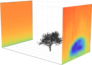
The estimation of the drag force is performed by applying the principle of momentum and mass conservation on a control volume of air. The control volume is delimited by two vertical planes perpendicular to the mean wind direction; one upstream of the tree called the inlet, and one downstream of the tree called the outlet (see figure 3). In addition to these planes, the volume is confined by a surface consisting of streamlines of the mean flow emanating from the inlet plane and ending on the outlet plane, forming a streamtube. The advantages of this choice of volume is that all momentum fluxes from the mean velocity field goes through the inlet and outlet planes. We will now go through this concept in more detail, considering an arbitrary, steady, control volume  $V$ that encapsulates the tree. The boundary surface of this closed volume is denoted as
  $A = \partial V$ and the outward normal vector as
  $\boldsymbol {n}$. The fluctuating but statistically stationary wind field
  $\tilde {\boldsymbol {u}}$, can be decomposed into a mean and fluctuations
  $\tilde {\boldsymbol {u}} = \boldsymbol {u}+\boldsymbol {u}'= \boldsymbol {u}(\boldsymbol {x})+\boldsymbol {u}'(\boldsymbol {x},t)$ such that the ensemble mean of the instantaneous fluctuations is zero
  $\left \langle \boldsymbol {u}'\right \rangle = \left \langle \boldsymbol {u}'(\boldsymbol {x},t)\right \rangle =0$. All other variables can be decomposed similarly. Here,
  $\boldsymbol {x}$ is the position vector defined in a three-dimensional Cartesian coordinate system, whose
  $x$-axis is aligned to the wind direction. Incompressibility,
  $\boldsymbol {\nabla } \boldsymbol {\cdot } \tilde {\boldsymbol {u}} = 0$ and constant air density
  $\rho$, implies
 \begin{equation} \int_V \rho \boldsymbol{\nabla} \boldsymbol{\cdot} \tilde{\boldsymbol{u}} \,\textrm{d} V = \int_{A} \rho \boldsymbol{n} \boldsymbol{\cdot} \tilde{\boldsymbol{u}} \,\textrm{d}A =\int_A \rho n_i \tilde{u}_i \,\textrm{d} A = 0 , \end{equation}
using the divergence theorem and the convention of summation over repeated indices (see Kundu, Cohen & Dowling Reference Kundu, Cohen and Dowling2012, chap. 4.2). The rate of change of the momentum inside the control volume can be written as the sum of the transport of momentum into the volume and the integral of all body forces including pressure gradient forces (here we ignore gravity)
 \begin{equation} \frac{\textrm{d}}{\textrm{d} t} \int_V \rho \tilde{\boldsymbol{u}} \,\textrm{d} V ={-} \int_A \rho \tilde{\boldsymbol{u}} n_j \tilde{u}_j \,\textrm{d} A + \tilde{\boldsymbol{F}} - \int_V \boldsymbol{\nabla}\tilde{p} \,\textrm{d} V, \end{equation}
where  $\tilde {\boldsymbol {F}}$ is the sum of all other body forces (see Kundu et al. Reference Kundu, Cohen and Dowling2012, chap. 4.4 and examples therein). Because of stationarity, the mean of the left-hand side is zero. The mean of the integrand inside the first term on the right-hand side is
  $\rho \left \langle \tilde {u}_i n_j \tilde {u}_j\right \rangle = \rho u_i n_j u_j + \tau _{ij} n_j$, where the Reynolds stress is defined as
  $\tau _{ij} = \rho \left \langle u'_i u'_j\right \rangle$. The average of equation 2.3 can be used to determine the mean force
 \begin{equation} F_i =\int_A \rho u_i u_j n_j \,\textrm{d} A + \int_A \tau_{ij} n_j \,\textrm{d}A + \int_A p n_i \,\textrm{d} A. \end{equation}
In principle, the force on the tree can be calculated by measuring fluid quantities on the surface  $A$. However, experimentally, we were not able to assess all the terms. Our experimental strategy is to choose a volume
  $V$ which is limited by two areas on vertical planes upstream and downstream from the tree, denoted as
  $A_{inlet}$ and
  $A_{outlet}$, respectively. The two vertical areas are assumed to be connected by mean streamlines, so
  $A = A_{inlet} + A_{outlet} +A_{tube}$ (see figure 3). This choice has the advantage that only the inlet and outlet terms, not the tube term since here
  $n_j u_j = 0$, contribute to the first term of the force. In order to proceed, we make the following assumptions:
(i) By using continuity (2.2) we are able to choose
 $A_{inlet}$ and $A_{outlet}$ such that the inflow mass rate equals to the outflow and the edges of the two areas are connected by streamlines.
(ii) The contribution of the second term on the right-hand side of (2.4), which describes the turbulent fluxes of momentum through the surface, can be neglected. The impact of this assumption is assessed and discussed in § 3.5.
(iii) The pressure term can be ignored. The inlet and outlet are sufficiently far away from the tree to have the ambient pressure and the tube walls are sufficiently parallel to the upstream flow direction (the
$x$-axis) not to contribute significantly to the mean force.(iv) The drag force
$F_d$, i.e. the force exerted on the tree by the wind, is equal to $-F_1$.


Figure 3. Top (a) and side (b) views of the control volume used in this study. The tree (black), the scanning plane (grey solid line) and the up- and downwind sonic anemometers (denoted as x and +, respectively). The minor and major axes of the inlet and outlet areas are denoted  $a_{inlet}$,
  $a_{outlet}$ and
  $b_{inlet}$ and
  $b_{outlet}$.
Based on the ratio between the width and the height of the crown ( $8.0/4.5 = 1.77$), we approximate the shape of
  $A_{outlet}$ as an ellipse. The three-dimensional control volume is then defined as a streamtube with an elliptical cross-section centred around the centre of gravity of the aerodynamic deficit. The control volume extends in the streamwise direction from the upwind meteorological mast (
 $x/H=-2.3$) to the scanning plane (
 $x/H=1.3$) of the short-range WindScanner (see figure 3).
The continuity equation (2.2) can thus be written
 \begin{equation} \int_{A_{inlet}} \rho u \,\textrm{d}A = \int_{A_{outlet}} \rho u \,\textrm{d}A, \end{equation}
where  $u = u_1$, and with all our assumptions the momentum equation (2.4) simplifies to
 \begin{equation} F_d = \int_{A_{inlet}} \rho u^2 \,\textrm{d}A - \int_{A_{outlet}} \rho u^2 \,\textrm{d}A. \end{equation}
The first of the two equations above allow us to adjust the inlet and outlet areas such that the net flow through the tube walls is zero. Once these areas are fixed the second permit us to estimate the drag force.
2.3. Wind measurements
In order to acquire measurements of the wind field in the outlet area of the control volume, the three short-range WindScanner wind lidar instruments were used (figure 1). The instruments were programmed to acquire measurements within a rectangular vertical plane that was parallel to the  $y$-axis at a distance of 8.5 m (
 $1.3H$) from the tree in the leeward direction. The plane was scanned synchronously by the three lidars using a trajectory that consisted of 30 vertical lines that extended from 1.5 m (
 $0.2H$) to 16 m (
 $2.5H$) and spanned from
  $-7.25$ m (
 $-1.1H$) to 7.25 m (1.1H) across the
  $y$-axis. The scanning duration of one plane was 26 s and the sampling rate of the instruments was 205 Hz. The acquired data, during each iteration of the scanning pattern, were partitioned in a grid of 900 rectangle cells with dimensions
  $0.5\ \textrm {m}\times 0.5\ \textrm {m}$. More information regarding the post-processing of the WindScanner data and the estimation of the wind component vector can be found in Angelou & Dellwik (Reference Angelou and Dellwik2020).
The two meteorological masts denoted M1 and M2 were equipped with 5 and 10 sonic anemometers, respectively. These observations were used to provide information regarding the free wind (M1 in figure 1) and to validate the resolved wind vector from the short-range WindScanner at ten different locations within the scanning pattern (M2 in figure 1). The upwind M1 mast had five sonic anemometers at the heights of 1.5, 4.0, 6.0, 8.5, 11.0 m a.g.l., installed on booms that pointed to the direction of  $200^\circ$, relative to the geographical North, which corresponds to the
  $-y$ direction in our coordinate system. The downwind M2 mast was equipped with two booms at each height, pointing in the directions of both negative and positive
  $y$. The heights of the booms of the M2 mast were at the same height a.g.l. as those on the M1 mast. A small offset in mounting height (
 $+0.15$ m) was applied in the installation of the booms that pointed in the positive
  $y$ direction due to mounting limitations. The sonic anemometer data were sampled at 20 Hz and post-processed by applying the flow distortion correction presented in Bechmann et al. (Reference Bechmann, Berg, Courtney, Jørgensen, Mann and Sørensensen2009) and Peña, Dellwik & Mann (Reference Peña, Dellwik and Mann2019). In addition, the sonic measurements were aligned to the horizontal plane, by using the scanned orientation of the instruments. The sonic anemometers and the wind lidars used different data acquisition systems. Their synchronisation was adjusted based on the cross-correlation between the wind speed time series acquired by the sonic anemometers and by co-located WindScanner measurements.
2.4. Inter- and extrapolation of inlet wind profile
For the wind direction sector examined in this study, the tree is expected to be located in an internal boundary layer (IBL) extending downwind from the shoreline. Therefore, a neutral wind profile observed at M1 cannot be simply logarithmic with respect to the local roughness. The profile is instead characterised by different vertical regions, where the influence from the upwind water surface and downwind low vegetation is blended (Garrat Reference Garrat1990).
The mean values, calculated over the whole examined period, the horizontal  $u$ and vertical
  $w$ wind speed, of the vertical tilt angle
  $\phi$ of the flow direction as well as of the friction velocity
  $u_\star$, measured by the sonic anemometers at M1 are shown in figure 4. Except for the top anemometer, the tilt angle shows close agreement with the terrain inclination (
 $2.7^{\circ }$). The
  $u_\star$ profile shows a systematic decrease with height, which is in accordance with the expected structure in the lowermost part of the IBL (Dellwik & Jensen Reference Dellwik and Jensen2000). The expected deviation from an equilibrium logarithmic profile can also be seen in figure 4(a), where the two grey lines, representing logarithmic fits to the data for
  $z\geqslant 1.5$ m (dashed line) and
  $z\geqslant 4$ m (solid line), fail to fit all observations. Instead, we use the more flexible wind profile model suggested by Högström (Reference Högström1988)
 \begin{equation} u(z)= u_o + A \ln z + B \ln^2 z, \end{equation}
where  $u_o$,
  $A$,
$A$,  $B$ are fitted parameters and
  $z$ the height. The application of this model (
 $u_o=5.49\ \mbox {ms}^{-1}$,
  $A = 3.00$,
  $B = -0.50$, black line in figure 4(a)) shows a close agreement with all observed wind speeds.

Figure 4. Mean measured profiles of (a) the horizontal wind speed in five different heights (black dots) and the three models of vertical profile (A: logarithmic profile ( $z \geqslant 1.5$ m) (dashed grey), B: logarithmic profile (
 $z\geqslant 4$ m) (solid grey) and C: profile based on the model suggested by Högström (Reference Högström1988) (solid black). (b) The vertical component of the wind vector, (c) the tilt angle and (d) of the friction velocity. The dashed line corresponds to the lower and higher limits of the tree crown (
 $H_c = 4.5$ m).
2.5. Case studies
Figure 5(a), shows the distribution of inlet wind directions for the whole experiment using data from the sonic anemometer at 4 m on the M1 mast. The averaging time of the wind data is 26 s, which corresponds to the plane scanning period. Out of these data, only periods that were characterised by a wind direction between  $285^\circ$ and
  $295^\circ$ were selected for the evaluation of the momentum deficit method. For this sector, a histogram of the acquired wind speeds is shown in figure 5(b). The corresponding synchronised WindScanner observations over the outlet plane were identified and subsequently grouped based on the mean wind speed.

Figure 5. Histograms of the mean wind direction (a) over the time period examined in this study (left) and the mean wind speed of the direction sector  $285^\circ \leqslant a < 295^\circ$ (b). The averaging period corresponds to the iteration time of a scanning plane. The dashed line in the wind speed histogram represents the threshold criterion applied to the selection of the cases used in this study.
In table 1, information regarding the amount of data and the wind conditions for the cases investigated in this study, are presented. The table also presents the parameters of the upwind profile (based on the model presented in (2.7), as well as, an estimation of the spanwise displacement of the wake  $d_y$ at the scanning plane, using the equation
 \begin{equation} d_y=y_{sp}\cdot \tan (290^\circ{-} \alpha), \end{equation}
where  $y_{sp}=8.5\ \textrm {m}$ is the distance between the tree and the scanning plane and
  $\alpha$ is the mean wind direction of the ensemble of each case.
Table 1. Wind conditions during the selected case studies, where  $N$ is the number of the scans realised,
  $U_{{bin}}$ is the
  $1\text {-}\textrm {ms}^{-1}$ range between the minimum and maximum wind speeds in a bin,
  $u$ and
  $\sigma _{{u}}$ are the mean and standard deviation of the streamwise wind and
  $\alpha$ and
  $\sigma _{\alpha }$ are the mean and standard deviation of the wind direction,
  $d_y$ the expected displacement of the center of the wake;
  $A$,
$A$,  $B$ and
  $u_o$ are the fit parameters of the upwind profile using (2.7).

2.6. Drag force reference measurement
A reference drag force was derived from an in situ sensor (strain gauge) mounted at the bottom of the stem. This strain gauge was installed on a calliper-shaped transducer in order to increase the observational sensitivity (Blackburn Reference Blackburn1997), facing the upwind M1 mast in the direction of  $-x$. The strain gauge observations were post-processed to estimate the bending moment over the entire tree, following the methodology presented in Angelou et al. (Reference Angelou, Dellwik and Mann2019). The measured strain is converted to a bending moment via calibration to a known static load. In this study, the calibration of the strain gauge was performed at an earlier stage when the tree's crown was fully developed, and since the tree is a living organism, small changes in calibration due to different states of the crown could be a source of a systematic bias (Gardiner et al. Reference Gardiner, Stagey, Belcher and Wood1997). Finally, the drag force is estimated using the ratio of the measured bending moments to the corresponding lever arm (
 $z_f$). In this step it is assumed that the wind load distributed over the frontal area of the crown of the tree can be expressed by one force exerted at a height that corresponds to the bending moment lever arm.
The lever arm should be dependent on the distribution and density of the tree elements, here expressed via the plant area density (PAD) of the tree. We estimated  $z_f$ using the centroid of the PAD weighted with the upwind wind profile
 \begin{equation} z_f = \frac{\sum_{z=0}^{z=H} PAD(z)u(z)z}{\sum_{z=0}^{z=H}PAD(z)u(z)}, \end{equation}
where  $u(z)$ is the inlet wind profile ((2.7) and figure 6) and
  $PAD(z)$ was taken from Dellwik et al. (Reference Dellwik, van der Laan, Angelou, Mann and Sogachev2019), who used high-detail terrestrial lidar scans of 1–2 cm resolution to create a summer and winter PAD model of the tree. The scans for the PAD model were taken during either full-leaf summer condition or bare crown winter condition, and hence neither is a perfect match for the tree in the autumn abscission phase. The estimated lever arm of the tree during the summer and winter was 3.93 m and 3.90 m, respectively. Since the tree had already lost a significant number of leaves (figure 2, centre) the
  $z_f = 3.90$ m was used to calculate the drag from the bending moment.

Figure 6. Vertical profile of the mean streamwise component of the six cases of different wind speeds as measured by the short-range WindScanners (blue) and up- and downwind sonic anemometers (red and black, respectively). A model of the up-wind profile is also presented in a thick red line. The error bars and the light blue region correspond to one standard deviation about the mean for the case of the sonic and WindScanner measurements, respectively. The grey line corresponds to the tree height.
For the bending moment measurements, we used strain gauge data from a wider wind direction sector,  $275^{\circ }$–
 $305^{\circ }$, than for the selection of wind data in the six cases defined above. The wider wind direction interval was necessary in order to provide sufficient data points to determine the functional relationship between drag force and wind speed. The resulting data set consisted of 250 1 min values of strain that were acquired for a wind speed interval between 5.6 and
  $13.9\ \textrm {ms}^{-1}$.
3. Results
3.1. Wind profile analysis
In figure 6, the vertical profile of the streamwise component in the wake ( $y/H$=0) is presented together with the corresponding upwind profile, for each of the six wind speed cases (table 1). It can be observed that, in most of the cases, the upwind and downwind profiles for
  $z/H \geqslant 1.2$ coincide. An exception is observed for case V, where the outlet wind speed is 6 % lower than the corresponding upwind profile. In the cases I–IV the wind speed deficit is concentrated in the range
  $0.2 \leqslant z/H \leqslant 1.2$. A different trend is exhibited in the profile of the sixth case, which corresponds to the highest wind speed, in which the wind speed deficit is observed to extend up to a height of 1.8
 $H$. A local minimum of the deficit is found in all the profiles, in the region
  $0.6 \leqslant z/H \leqslant 0.9$, which is attributed to an increase of the porosity of the crown in the area.
The accuracy of the three WindScanners in measuring the streamwise component of the wind is evaluated using the data from the ten sonic anemometers of the M2 mast as a reference (figure 7). The result of a linear fit shows that the measurements of the two instruments are in good agreement (mean absolute error:  $0.36\ \textrm {ms}^{-1}$) and highly correlated (
 $R^2=0.98$). The high correlation shows that the small measuring offset between the two instruments is wind speed independent.

Figure 7. Scatter plot of the mean streamwise component measured in the wake of the tree by the short-range WindScanners ( $u_{ws}$) versus the corresponding sonic anemometer (
 $u_{sonic}$) measurements. The dashed line corresponds to the identity line. The linear fit over the ensemble of all the cases is presented with a black line.
3.2. Determination of the control volume's outlet area
An example (case II) of the scanned wind field over the plane in the outlet is shown in figure 8(a). It is observed that the wind speed is strongly reduced in the wake, and that this reduction is inhomogeneous in the crown area, such that less wake deficit is observed in areas with higher porosity in the left side of the crown and a higher deficit is observed where the crown appears more dense (see figure 2b). The black dashed line roughly indicates the outline of the tree, projected onto the vertical plane of the outlet.

Figure 8. Example (case II) of the mean (a) measured  $u$ and (b) normalised by the upwind profile
  $\hat {u}$ streamwise component of case II. The vertical and horizontal profiles that intersect at the aerodynamic centre, depicted by white dashed lines in (b) are presented in (c) and (d), respectively.
In order to determine the centre of  $A_{outlet}$, we start by normalising the WindScanner observations in the wake of the tree with observations at the same
  $y$ and
  $z$ positions on the inlet plane. For the normalisation step, the upwind conditions are considered horizontally homogeneous and thus the wind profile measured by the M1 meteorological mast is characteristic of the vertical upwind flow across the whole area covered by the scanning pattern. This step is illustrated in figure 8(b), where the normalised wind data in the plane are denoted
  $\hat {u}$. When normalising, it becomes clear that the wake extends outside the black dashed line, which shows that the wake expands between the tree and the scanning plane. Next, we identify the location of the wake centre.
For this step, we select only those grid cells in the outlet plane, where  $\hat {u} < 0.8$. The centre position of the wake, denoted
  $\{y_c, z_c\}$, is then calculated as the centre of gravity of the wind speed deficit, according to
 \begin{equation} y_c = \frac{\sum_{i=1}^N y[i] \hat{u}[i]}{\sum_{i=1}^N \hat{u}[i]}\quad \mbox{and}\quad z_c = \frac{\sum_{i=1}^N z[i] \hat{u}[i]}{\sum_{i=1}^N \hat{u}[i]}, \end{equation}
where  $N$ is the total number of the chosen grid cells.
The calculated spanwise offsets ( $y_c$) of the wake centre, which are presented in table 2, are found to be very similar to the predicted displacement of the wake due to the horizontal wind direction in all cases, except case VI (
 $d_y$ in table 1), where a difference of 0.5 m, corresponding to 0.08
 $H$, is found. The height (
 $z_c$) of the wake centre is found to be within 4.3–4.5 m for all the cases. An example of the wake centre location is shown in figure 8. The horizontal and vertical wind profiles through the aerodynamic centre are shown both for the measured (blue) and normalised (black) values in figures 8(c) and 8(d).
Table 2. Ratio between the inlet and outlet areas of the control volume ( $A_{inlet}/A_{outlet}$) for each of three streamline divergence patterns defined in figure 10 and for each of the wind speed cases presented in table 1;
  $\{y_c,z_c\}$ are the spanwise and vertical coordinates of the location of the wake centre,
  $d_o$ is the scaling parameter of the inlet area for which the conservation of the mass rate is satisfied.

The outlet area was finally calculated as an ellipse centred around the  $\{y_c, z_c\}$ position for each of the six wind speed cases. The dimensions of the outlet area were afterwards selected on the basis that its area should be within the margins of the scanning plane, while keeping the same ratio between the minor and major axes as that of the crown shape. Based on these two considerations the outlet area was equal to
  $61 \ \textrm {m}^2$, with
  $a_{outlet} = 6.0\ \textrm {m}$ and
  $b_{outlet} = 3.5\ \textrm {m}$.
3.3. Determination of the inlet area of the control volume
According to mass conservation, the mass flow through the outlet should match that of the inlet (2.2). Since the tree decelerates the flow, the area of the inlet should therefore be smaller than that of the outlet. Due to the distance of the crown from the ground, the inhomogeneous geometric shape of the frontal area of the crown and of the porosity of the tree, it is not possible to predict whether the streamlines of the free flow will diverge homogeneously in all directions or whether they will tend to diverge more above or around the tree. In order to assess the impact of the shape of the inlet surface on the momentum deficit estimation, we investigate three different divergence patterns according to which, the streamlines: (i) are homogeneously expanding around an ellipse (denoted as P1), (ii) tend to diverge mainly above and below (denoted as P2) or (iii) diverge mainly in the horizontal direction (denoted as P3). The three patterns are in presented in figures 9(a), 9(b) and 9(c), respectively.

Figure 9. Three patterns of streamline divergence caused by the presence of the tree, according to which the streamlines are considered to (a) diverge homogeneously radially from the centre of the tree, (b) diverge mainly above and below the tree and (c) diverge mainly on the sides of the tree.
The estimation of the inlet area for each of the three streamline divergence patterns was performed using the following procedure. First, the inlet and outlet areas were defined as two ellipses, described by the following equations:
 \begin{equation} \frac{(y-y_c)^2}{(a_{inlet}-d_a)^2}+\frac{(z-z_c)^2}{(b_{inlet}-d_b)^2}=1\quad \mbox{and}\quad \frac{(y-y_c)^2}{a_{outlet}^2}+\frac{(z-z_c)^2}{b_{outlet}^2}=1, \end{equation}
where  $a_{inlet}$,
  $b_{inlet}$ and
  $a_{outlet} = 6.0\ \textrm {m}$,
  $b_{outlet} = 3.5\ \textrm {m}$ are the major and minor semi-axes, of the inlet and outlet areas, respectively. The parameters
  $d_a$ and
  $d_b$ are used to add a weight to the diverging streamlines (homogeneous
  $d_a$ =
  $d_b$, mainly above and below
  $d_a$ =
  $2d_b$ and mainly to the sides
  $d_a = d_b/2$). The parameters
  $y_c$ and
  $z_c$ are the coordinates of the centre of the ellipse.
Subsequently, the following steps were performed:
(i) Decrease the area of inlet by a parameter
$d_b = d$, where $d$ varied between 0.0 and 1.5 m, with a step of 0.25 m.(ii) Apply a spatial two-dimensional linear interpolation in the planes, where the inlet and outlet areas was located.
(iii) Estimate the mass rate imbalance
$\Delta \dot {{m}}$ through the inlet and outlet using (2.5).(iv) Use an inverse function to estimate the zero crossing
$d_0$ of the interpolated function.


In figure 10, the mass rate imbalance for cases I–VI as a function of the ratio between the inlet and the outlet area is presented for the three streamline divergence patterns P1–P3 defined above. The results without normalisation are shown in panels (a,c,e), whereas panels (b,d,f) show the normalised results after division by  $\rho U_{inlet}\ (4\ \textrm {m})$.

Figure 10. Measured (a,c,e) and normalised (b,d,f) by the mean wind speed, difference of the mass rate between the inlet and outlet vertical elliptical planes, for different dimensions of the inlet plane for three different streamline divergence patterns; P1: (a)–(b), P2: (c)–(d) and P3: (e)–(f).
It is observed that the conservation of mass rate is satisfied when the inlet area is 72 %–77 % of the outlet area. No clear wind speed dependence is observed, while the  $\Delta \dot { {m}}$ dependence on the ratio between the inlet and outlet areas shows the same trend for all the wind speeds (figure 9b,d,f). The resulting values of
  $d_0$ and of the corresponding
  $A_{inlet}/A_{outlet}$ ratio are presented in table 2.
3.4. Estimation of drag force
The results of the drag estimation based on the momentum deficit are similar for all three streamline divergence patterns (see figure 11a). Prior the integration over the inlet and outlet surface areas, the spacing between adjacent vectors in the two planes was reduced from 0.5 m to 0.01 m, using a two-dimensional linear interpolation. This step was performed in order to ensure the mass flows through the two areas are identical.

Figure 11. Estimated values of the wind drag based on (a) the momentum deficit for three different patterns (P1, P2 and P3) of streamline divergence and (b) the 1 min mean bending moment measurement. Comparison between the drag estimation using the P1 streamline pattern and (c) the bending moment and (d) the wind load on the same tree during the summer (long dashed grey line) and the winter (short dashed grey line) based on the results presented in Angelou et al. (Reference Angelou, Dellwik and Mann2019).
In the wind speed range examined in this study ( $7\text {--}12\ \textrm {ms}^{-1}$) the drag increases from approximately 530 to 1500 N. A nonlinear model fit of a power law function
  $F_d=b u^n$, gives exponents of 1.82, 1.87 and 1.78, for the P1, P2 and P3 patterns, respectively. The model was applied to the data of all the cases, excluding case V (
 $u= 11.05\ \textrm {ms}^{-1}$). The reason of the exclusion is the difference between the upwind and wake profiles in the heights above
  $z/H \geqslant 1.2$ (figure 6e), which leads to an overestimation of the drag.
The choice of fitting an exponent rather than imposing a quadratic dependence between the drag and the wind speed, as in (1.1), is justified by the characteristics of the tree response under wind loading. Vogel (Reference Vogel1984) has observed that leaves and brunches exposed to wind tend to reconfigure their shape and orientation and therefore cannot be considered as bluff bodies. An extensive review of the processes that have an impact on the functionality between the wind speed and the drag on vegetation can be found in Gosselin (Reference Gosselin2019).
The estimated values of the drag using the method based on the momentum deficit are found approximately equal to the ones measured by the reference method (figure 11b). The mean absolute difference between the two methods, over the wind speed range  $7\text {--}12\ \textrm {ms}^{-1}$ (after excluding case V (table 1)) is found to be equal to 4 %, 1 % and 5 % for each of the P1, P2 and P3 streamline divergence patterns, respectively. A comparison is presented in figure 11(c).
In addition, both methodologies result in the same drag exponent ( $n = 1.8$). This value is between the values 1.6 and 1.9 that have been estimated on the same tree, during periods where the crown was fully developed and leafless, respectively (Angelou et al. Reference Angelou, Dellwik and Mann2019) (see figure 11d). This result should be expected since, during the period examined in this study, the leaves of the tree were in the abscission stage and thus the crown had lost part of its foliage. Based on the wind speed exponent (i.e. 1.8) the Vogel exponent is equal to
  $-0.2$. This suggest that mature open-grown oak trees during the abscission stage present a lower reconfiguration than has been observed in young conifer and deciduous trees (Moore & Maguire Reference Moore and Maguire2005; Kane & Smiley Reference Kane and Smiley2006; Whittaker et al. Reference Whittaker, Wilson, Aberle, Rauch and Xavier2013).
3.5. Impact of the turbulence stresses on the drag estimation
The estimation of the drag force using the momentum deficit has been performed assuming that the contribution of the turbulence stresses in (2.4) is negligible. In order to investigate the validity of this hypothesis we use the data acquired in the wind speed range  $6.5\text {--}7.5\ \textrm {ms}^{-1}$ (case II in table 1). This data set is formed by an ensemble of 43 scanning pattern iterations, which is equivalent to a period of 17 min. This period is adequate for the estimation of the second-order statistics of the wind, through which we can quantify the contribution of the normal stresses to the conservation of momentum. This is achieved by including two more terms in (2.6)
 \begin{equation} F_d = \int_{A_{inlet}} \rho u^2 \,\textrm{d}A - \int_{A_{outlet}} \rho u^2 \,\textrm{d}A + \int_{A_{inlet}}\tau_{11} \,\textrm{d}A - \int_{A_{outlet}}\tau_{11}\,\textrm{d}A. \end{equation}
 The contribution of the Reynolds stresses in the inlet area is estimated by the profile of the streamwise variance  $\langle u'u' \rangle$, which is presented in figure 12(a). By assuming horizontal homogeneity, the streamwise variance across an inlet plane is calculated using a linear inter- and extrapolation (figure 12b).

Figure 12. (a) Vertical profile at  $y/H=0$, of the
  $\langle uu \rangle$ measured at the upwind distance of
  $x/H=-2.3$ (red) and at the downwind distances of
  $x/H=-1.5$ (black) and
  $x/H=-1.3$ (blue, scanning plane). (b) Linearly interpolated plane of the upwind
  $\langle u'u' \rangle$ based on the fit presented in (a) (solid red line) and (c) measurement of
  $\langle u'u' \rangle$ in the wake of the tree.
In the plane of the outlet area the WindScanner observations reveal a thin layer with high variance along the edges of the crown (figure 12c). The thickness of this layer can be seen in the vertical profile of  $\langle u'u' \rangle$ at the centre of the plane (
 $y/H$ = 0), where a strong increase in
  $\langle u'u' \rangle$ is found within the height range
  $0.8 \leqslant z/H \leqslant 1.1$.
The measured  $\langle u'u' \rangle$ from the sonic anemometers is generally higher than the one calculated from the short-range WindScanner observations (figure 12a). This underestimation is expected since the wind lidar instruments measure over a longer probe length than the sonic anemometers, which results in the partial filtering of high frequency turbulence (Angelou et al. Reference Angelou, Mann, Sjöholm and Courtney2012). An exception is observed in the measurements of the sonic anemometer at 6 m (
 $z/H=0.9$) that is within the width of the layer of high
  $\langle u'u' \rangle$. This observation could be explained either by random noise in the WindScanner data that results in a bias of the second-order estimation, or due to a small offset in the vertical position of the scanning plane.
By applying equation (3.3) in the same inlet and outlet areas as described in §§ 3.2 and 3.3 we find that the inclusion of the Reynolds stresses results in a decrease of the drag by 5.0 %. Near identical results, using similar normalised distances from the vertical planes to the object, have been reported by Terra et al. (Reference Terra, Sciacchitano and Shah2019) in the case of a wind tunnel study of the drag on a full-scale bicycling mannequin model.
4. Discussion
In this study, the estimation of the drag based on the observed momentum deficit required the construction of a control volume that enclosed the tree. While the length of the volume was imposed by the location of the in situ measurement devices (sonic anemometers) and of the scanning plane of the WindScanners, a choice had to be made regarding the shape and the size of the cross-section of the control volume. Besides an ellipse, two more shapes were tested as cross-sections, a square and a rectangular ( $\textrm {height}/\textrm {width} = 0.8$) area centred on the wake deficit centre. The analysis presented in this study was performed for all the three shapes and for a varying size of the inlet and outlet areas. The results of the rectangular and square cross-sections were found to be very close to the ones from the ellipse, however, they showed a larger variation in comparison to the reference method. This is attributed to the spatial variation of the inflow speed, which introduces a bias in the estimation of the momentum. For this reason, the ellipse was selected as the most appropriate to construct the control volume used in this study. When reducing the size of the outlet area by letting the minor and major axes be 0.5 m shorter, part of the wake is excluded, leading to an underestimation of the drag force. In summary, the outlet size and shape should be selected such that the whole wake is covered, while avoiding large areas outside the wake.
4.1. Uncertainties
The comparison of the two different methods for estimating the drag force on a full-scale tree shows a difference between the two methods of up to 10.0 % (when the turbulence stresses are taken into account). This difference between the reference and momentum deficit method could be attributed to the assumptions that were made for the formulation of the conservation of momentum. For example, since the scanning plane is close to the tree ( $x/H=1.3$) a pressure imbalance between the inlet and outlet surfaces of the control volume could be expected (corresponding to a violation of assumption (iii), see § 2.2). The location of the inlet and outlet planes was selected due to limitations of space in the lee side of the tree, however, ideally, the scanning plane should be further away. Furthermore, it was assumed that the momentum transport through the sides of the streamtube is negligible.
Another possible explanation for the discrepancy between the reference and momentum deficit methods concerns an error in the reference method. Here, we have followed the methodology presented in Angelou et al. (Reference Angelou, Dellwik and Mann2019), in which the calibrated bending moment from the strain gauges is translated to a drag force using an estimated lever arm. The estimation of the lever arm is challenging in a three-dimensional complex object, such as a mature tree. In this study, the lever arm is estimated to 3.9 m using the product of the vertical profiles of PAD and wind speed. However, another possible choice of lever arm is the height of the wake centre (table 2), which is found to be approximately 0.5 m higher. A third possibility, which was used in Angelou et al. (Reference Angelou, Dellwik and Mann2019), is to set the lever arm equal to the geometrical centre of the tree, which resulted in a lever arm estimate of 3.8 m. An underestimation of the lever arm would lead to the overestimation of the drag force using the strain gauge methods and vice versa. Given its uncertainty, this parameter alone could also explain the discrepancy between the two methods used in this study. Although uncertain, this discussion highlights that by choosing the height of the maximum wake deficit as the lever arm, the bending moment – and not only the drag force – can be estimated using the momentum deficit approach.
4.2. Future perspectives
This study was based on using three scanning lidars to measure the wind vector on a plane in the near-wake region. The use of three additional lidars to monitor the upwind conditions would improve the estimation of the momentum deficit by mitigating errors attributed to the assumption of the horizontal homogeneity of the inflow.
The presented method would, in principle, also be valid for a group of trees as well as other objects. For an extension to larger objects, turbulent fluxes through the sides of the control volume could, however, contribute significantly to the momentum balance. This contribution can be minimised by avoiding sites with high ambient turbulence. Alternatively, these fluxes should be measured by using more scanning wind lidars.
The results of this study demonstrate the feasibility of quantifying the drag force by objects using a methodology that relies on wind field observation from scanning Doppler lidars. This method can contribute to meteorological and wind engineering research areas, especially for determining the drag of objects that are difficult to downscale or move to a wind tunnel. Furthermore, an advantage of this method is that it does not require detailed information about the geometry or the physical characteristics of a surface obstacle and allows for the study of the surrounding flow in its natural environment.
5. Conclusion
The flow field in a cross-section of the wake behind a solitary open-grown oak tree was measured with a high spatial resolution using three synchronised wind scanning lidars. The measurements were acquired during a short field experiment during the autumn of 2017, and the analysis is limited to a narrow wind direction interval, where the flow is near perpendicular to the scanning plane. Based on these observations, we presented a new way of estimating the drag force on the tree and compared it to a reference method using observations from a tree-mounted sensor. Contrary to the reference, the new method does not require a detailed description of the complex tree structure. Instead, the drag was estimated by applying the momentum conservation principle to a control volume along streamlines, where the streamlines were determined using the mass conservation equation.
The method was applied to six different wind speed cases ( $7\text {--}12 \ \textrm {ms}^{-1}$) and showed that the exponent of the drag force–wind speed relation was equal to 1.8. The same exponent was found using the measurements from the reference method. Further, a small discrepancy of 1 %–5 % between the two methods was found. This discrepancy increases by approximately 5.0 % when the turbulent transport through the inlet and outlet of the control volume is taken into account. Two likely sources of error have been identified: the force estimation based on the tree-mounted bending moment sensors may be overestimated due to difficulties in converting the measured bending moment to a drag force, and the pressure terms in the momentum deficit approach may not be negligible. The presented work points to new possibilities in estimating the drag on complex objects in the real atmosphere.
Acknowledgements
C.B.M. Pedersen and P. Hansen, research technicians in the Wind Energy Department of DTU, are acknowledged for their valuable support during the realisation of the experimental campaign.
Funding
This study is funded by the Independent Research Fund Denmark via The Single Tree Experiment project (Grant No. 6111-00121B).
Declaration of interests
The authors report no conflict of interest.


