1. INTRODUCTION
Laser induced breakdown spectroscopy (LIBS) is an analytical technique that is being applied in industry (Noll et al., Reference Noll, Bette, Brysch, Kraushaar, Monch, Peter and Sturm2001; Noll et al., Reference Noll, Begemann, Brunk, Connemann, Meinhardt, Scharun, Sturm, Makowe and Gehlen2014), environmental diagnostics (Bassiotis et al., Reference Bassiotis, Diamantopoulou, Giannoudakos, Kalantzopoulou and Kompitsas2001; Bulajic et al., Reference Bulajic, Cristoforetti, Corsi, Hidalgo, Legnaioli, Palleschi, Martins, McKay, Tozer, Wells, Wells, Harith, Salvetti, Tognoni, Green, Bates, Steiger and Fonseca2001), and biomedical research (Bassiotis et al., Reference Bassiotis, Diamantopoulou, Giannoudakos, Kalantzopoulou and Kompitsas2001; Singh & Rai, Reference Singh and Rai2001). In this technique a high-power pulsed laser is focused on the surface of a solid (Gomba et al., Reference Gomba, Angelo and Bertuccelli2001; Fichet et al., Reference Fichet, Menut, Brennetot, Vors and Rivoallan2003; Hafeez et al., Reference Hafeez, Sheikh and Baig2008; Baig et al., Reference Baig, Qamar, Fareed, Anwar-ul-Haq and Ali2012), liquid (Charfi & Harith, Reference Charfi and Harith2002; Fichet et al., Reference Fichet, Menut, Brennetot, Vors and Rivoallan2003; Mohamed, Reference Mohamed2007) or in the gaseous target (Hohreiter & Hahn, Reference Hohreiter and Hahn2005) to generate plasma. Elemental composition of any material can be obtained from the emission spectrum of the laser produced plasma (Cremers & Radziemski, Reference Cremers and Radziemski2006; Hahn & Omenetto, Reference Hahn and Omenetto2012). For the last couple of decades, LIBS technique has been used for the qualitative and quantitative analysis (Ciucci et al., Reference Ciucci, Corsi, Palleschi, Rastelli, Salvetti and Tognoni1999; Bassiotis et al., Reference Bassiotis, Diamantopoulou, Giannoudakos, Kalantzopoulou and Kompitsas2001; Fichet et al., Reference Fichet, Menut, Brennetot, Vors and Rivoallan2003; Winefordner et al., Reference Winefordner, Gornushkin, Correll, Gibb, Smith and Omenetto2004; Ahmed et al., Reference Ahmed and Baig2015; Ahmed & Baig Reference Ahmed, Iqbal and Baig2015) by the calibration curves method (Galbacs et al., Reference Galbacs, Gornushkin, Smith and Winefordner2001) and by the calibration free (CF) methods (Galbacs et al., Reference Galbacs, Gornushkin, Smith and Winefordner2001; Hohreiter & Hahn Reference Hohreiter and Hahn2005; De Giacomo et al., Reference De Giacomo, Dell'Aglio, De Pascale, Gaudiuso, Teghil, Santagata and Parisi2007a , Reference De Giacomo, Dell'Aglio, De Pascale, Longo and Capitelli b ; Tognoni et al., Reference Tognoni, Cristoforetti, Legnaioli and Palleschi2010; Unnikrishnan et al., Reference Unnikrishnan, Mridul, Nayak, Alti, Kartha, Santhosh and Gupta2012). In the calibration curve method, reference samples are needed for drawing the calibration curves between the emission lines intensities versus the known compositions. The composition of the unknown samples is then estimated by comparing the emission line intensity from the calibration curves (Bassiotis et al., Reference Bassiotis, Diamantopoulou, Giannoudakos, Kalantzopoulou and Kompitsas2001; Fichet et al., Reference Fichet, Menut, Brennetot, Vors and Rivoallan2003; Gupta et al., Reference Gupta, Suri, Verma, Sunderaraman, Unnikrishnan, Alti, Kartha and Santhosh2011; Unnikrishnan et al., Reference Unnikrishnan, Mridul, Nayak, Alti, Kartha, Santhosh and Gupta2012; Ahmed et al., Reference Ahmed, Iqbal and Baig2015). Limitation of this method is that, only samples with similar compositions can be analyzed quantitatively. However, in the CF-IBS method, no reference samples are needed (Gomba et al., Reference Gomba, Angelo and Bertuccelli2001; Burakov & Raikov, Reference Burakov and Raikov2007; Aguilera et al., Reference Aguilera, Aragon, Cristoforetti and Tognoni2009; Tognoni et al., Reference Tognoni, Cristoforetti, Legnaioli and Palleschi2010; Unnikrishnan et al., Reference Unnikrishnan, Mridul, Nayak, Alti, Kartha, Santhosh and Gupta2012). For the quantitative analysis of a sample, the plasma needs to be optically thin (Unnikrishnan et al., Reference Unnikrishnan, Alti, Kartha, Santhosh, Gupta and Suri2010), and fulfills the local thermodynamic equilibrium (LTE) condition (Cristoforetti et al., Reference Cristoforetti, Giacomo, Dell'Aglio, Legnaioli, Togoni, Palleschi and Omenetto2010). In the one-line calibration free LIBS (OLCF-LIBS) method, only a single spectral line is used to measure the elemental composition. Whereas, to draw a Boltzmann plot for the determination of plasma temperature and composition, at least four to five optically thin spectral lines are required. However, in the case of trace elements, it is always difficult to find sufficient number of optically thin lines, which limits the use of the Boltzmann plot method for the quantitative analysis of the trace elements in the target material. To overcome this difficulty Gomba et al. (Reference Gomba, Angelo and Bertuccelli2001) developed a new CF-LIBS technique in which concentration of the elements can be estimated by comparing the theoretically obtained electron density and the ratio of the number densities of neutral and the singly ionized species of the same elements as well as of the different elements with the experimentally measured electron densities. However, accurate values of the electron density n e and temperature T e are important in CF-LIBS. The electron temperature T e can be deduced from the Boltzmann plot method (Joseph et al., Reference Joseph, Xu and Majidi1994; Gomba et al., Reference Gomba, Angelo and Bertuccelli2001; El Sherbini & Saad Al Aamer, Reference El Sherbini and Saad Al Aamer2012) and electron number density n e can be calculated from the Stark broadening of the spectral lines (Borgia et al., Reference Borgia, Burgio, Corsi, Fantoni, Palleschi, Salvetti, Squarcialupi and Togoni2000; Cremers & Radziemski, Reference Cremers and Radziemski2006) or by the Saha–Boltzmann equation (Borgia et al., Reference Borgia, Burgio, Corsi, Fantoni, Palleschi, Salvetti, Squarcialupi and Togoni2000; Andrzej et al., Reference Andrzej, Palleschi and Israel2006; Unnikrishnan et al., Reference Unnikrishnan, Mridul, Nayak, Alti, Kartha, Santhosh and Gupta2012).
Copper (Cu) and nickel (Ni) are adjacent elements in the Period Table. The Cu–Ni alloy is highly resistant to corrosion therefore it is used in marine applications. A typical Cu–Ni alloy with 75% copper and 25% nickel is used in new strewn coins. The main objectives of the present work were to exploit the LIBS as well as other techniques for the quantitative analysis of the Cu–Ni alloy, which is used to make the Pakistani five rupee coin of year 2004 and to compare it with its certified composition. Quantitative results obtained using three LIBS-based techniques; OLCF-LIBS (Andrea et al., Reference Andrea, Pagnotta, Grifoni, Legnaioli, Lorenzetti, Palleschi and Lazzerini2015), SC-LIBS (Ciucci et al., Reference Ciucci, Corsi, Palleschi, Rastelli, Salvetti and Tognoni1999), CF-LIBS (Unnikrishnan et al., Reference Unnikrishnan, Mridul, Nayak, Alti, Kartha, Santhosh and Gupta2012) are compared with that obtained by the XRF, EDX, and LA-TOF techniques showing good agreement.
2. EXPERIMENTAL SETUP
The experimental details for recording the optical emission spectrum of the laser produced plasma are the same as described in our earlier papers (Hafeez et al., Reference Hafeez, Sheikh and Baig2008; Ahmed & Baig, Reference Ahmed and Baig2009; Baig et al., Reference Baig, Qamar, Fareed, Anwar-ul-Haq and Ali2012; Shaikh et al., Reference Shaikh, Kalhoro, Hussain and Baig2013; Ahmed et al., Reference Ahmed, Iqbal and Baig2015). In brief, for the ablation of the target sample we have used a high-power Q-switched Nd:YAG laser (Brilliant-B-Quantal, France) having 5 ns pulse duration and 10 Hz repetition rate. The laser pulse energy is about 850 mJ at 1064 nm and about 500 mJ at 532 nm. Using the LIBS software, the laser pulse energy can be changed by varying the Q-switch delay whereas the laser energy has been measured by an energy meter (Nova-Quantal, France). A quartz lens (convex) of 20 cm focal length was used to focus the laser beam on the target sample placed in air at an atmospheric pressure. The sample was placed on a rotating stage that was kept rotating around an axis; to prevent the formation of deep craters, to provide a fresh location of target sample for the energy single shot, for the improvement of reproducibility of mass ablation and to avoid the non-uniformly of the target. In order to prevent the air breakdown in front of the sample, it was necessary to keep the distance between the lens and the sample less than the focal length (<20 cm). The optical fiber (high – OH, core diameter about 600 µm) was used to collect the plasma radiation with a collimating lens (0°–45° field of view), which was placed normal to the laser beam. The emitted radiation was guided to the spectrometer through the fiber optics and then detected by the system software. There are four spectrometers each having width of 10 µm in the detection system (Avantes, Holand), which covers the wavelength range of 250–870 nm. To correct the emission signal, we subtracted the dark signal of the detector using the LIBS software. Three LIBS-based methods are employed for quantitatively analyzing the LIBS spectra, One line calibration LIBS (OLC-LIBS), self-calibration LIBS (SC-LIBS), and CF-LIBS. The same Pakistani five rupee coin of year 2004 was quantitatively analyzed by using the Bruker S8 Tiger X-ray fluorescence (XRF) spectrometer, by the EDX spectrometer attached with Quanta 450 FEG scanning electron microscope, and by a locally fabricated laser ablation/ionization time-of-flight mass spectrometer (TOF-MS).
3. RESULTS AND DISCUSSIONS
3.1. Emission Studies
The plasma on the surface of the sample was generated by focusing the beam of a Nd:YAG laser at 532 nm, pulse energy 130 mJ. As soon as the plasma is generated, the plasma plume expands perpendicular to the target surface and after a few micro seconds, it cools down. The emission from the plasma plume contains characteristics spectral lines of the constituent elements. The time delay of 2 µs between the laser pulse and the detection system was opted to reduce the continuum contribution. In Figures 1–3, the emission spectra of the laser produced Cu–Ni alloy plasma are presented covering the wavelength region from 200 to 700 nm. The major part of Figures 1–3 consists of spectral lines of copper and nickel as the alloy mainly contains these elements. The dominating lines belong to neutral copper and nickel. Besides, a couple of lines attached to the singly ionize copper and nickel are observed.
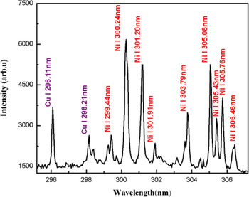
Fig. 1. Optical emission spectrum of the laser produced Cu–Ni alloy plasma covering the spectral region 295–307 nm. The spectral lines of Cu I and Ni I are assigned in the blue and red color, respectively.

Fig. 2. Optical emission spectrum of the laser produced Cu–Ni alloy plasma covering the spectral region 350–475 nm. The spectral lines of CuI, II and NiI, Ni II are assigned in blue and red color, respectively.
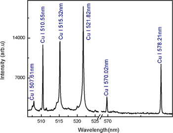
Fig. 3. Optical emission spectrum of the laser produced Cu–Ni alloy plasma covering the spectral region 506–579 nm. All the lines belong to neutral copper.
3.2. Determination of Plasma Temperature
We have determined the plasma temperature from the relative intensities of the emission lines of copper and nickel using the Boltzmann plot method (Borgia et al., Reference Borgia, Burgio, Corsi, Fantoni, Palleschi, Salvetti, Squarcialupi and Togoni2000). The observed emission spectra contain spectral lines of CuI at 296.11, 450.93, 453.96, 458.69, 510.55, 515.32, 570.02, 578.21 and 521.82 nm; and that of NiI at 490.44, 300.25, 301.20, 305.08, 339.30, 344.62, 345.85, 346.16, and 356.64 nm, which have been used to construct the Boltzmann plot to extract the plasma temperature. We have selected the optically thin lines in the Boltzmann plot that are free from self-absorption (Harilal et al., Reference Harilal, Shay and Tillah2005; De Giacomo et al., Reference De Giacomo, Dell'Aglio, De Pascale, Gaudiuso, Teghil, Santagata and Parisi2007a , Reference De Giacomo, Dell'Aglio, De Pascale, Longo and Capitelli b ; Cristoforetti et al., Reference Cristoforetti, Giacomo, Dell'Aglio, Legnaioli, Togoni, Palleschi and Omenetto2010). To validate the condition for the optically thin plasma from the observed emission spectrum, we have used the experimentally observed intensity ratio of various spectral lines of CuI and NiI and compared it with the ratio of their transition probabilities (Unnikrishnan et al., Reference Unnikrishnan, Mridul, Nayak, Alti, Kartha, Santhosh and Gupta2012). We used three pairs of lines in CuI at 515.32 and 521.82 nm, 470.45 and 529.25 nm, 510.55 and 515.32 nm; and one pair of lines of NiII at 254.66 and 251.163 nm. The experimentally observed and the theoretically calculated values agree with in 10% uncertainty, which supports the optically thin plasma assertion.
The atomic parameters of the selected lines were taken from NIST database that are listed in Table 1. The Boltzmann plots for copper and nickel are presented in Figure 4. The plasma temperatures have been extracted from the slopes of the straight lines, which yields the value for copper as 9535 ± 300 K and for nickel 9455 ± 300 K. The errors in the deduced plasma temperatures mainly come from the uncertainties in the transition probabilities and in the measurement of the line intensities. For the quantitative analysis, we have used an average value of the plasma temperature 9500 ± 300 K.

Fig. 4. Typical Boltzmann plots for estimating the plasma temperature. Emission lines from singly ionized Cu and Ni are used for obtaining temperature.
Table 1. Spectroscopic parameters of the emission lines of copper and nickel (NIST data base) to construct the Boltzmann plot.

3.3. Determination of Electron Number Density
One of the commonly used methods to calculate the electron number density is from the measured Stark broadening of neutral or singly ionized spectral lines. The electron number density (N e) is related to the full-width at half-maximum (FWHM) of a Stark broadened line as (Borgia et al., Reference Borgia, Burgio, Corsi, Fantoni, Palleschi, Salvetti, Squarcialupi and Togoni2000; Cremers & Radziemski, Reference Cremers and Radziemski2006):
 $$n_{\rm e} ({\rm cm}^{ - 3} ) = \left( {\displaystyle{{\Delta {\rm \lambda} _{{\rm FWHM}}^{\rm S}} \over {2{\rm \omega} _{\rm s} ({\rm \lambda}, T_{\rm e} )}}} \right) \times N_{\rm r}, $$
where
 $\Delta {\rm \lambda} _{{\rm FWHM}}^{\rm S}$
is the Stark contribution to the total line profile, ωs is the Stark broadening parameter, which is slightly wavelength and temperature dependent and its values are available in the literature, and N
r is the reference electron density, which is equal to 1016 (cm−3). The Stark line widths
$\Delta {\rm \lambda} _{{\rm FWHM}}^{\rm S}$
is the Stark contribution to the total line profile, ωs is the Stark broadening parameter, which is slightly wavelength and temperature dependent and its values are available in the literature, and N
r is the reference electron density, which is equal to 1016 (cm−3). The Stark line widths
 $\Delta {\rm \lambda} _{{\rm FWHM}}^{\rm S} $
of the spectral lines have been determined by deconvoluting the observed line profiles as a Voigt profile, which takes into account the instrumental width and the Doppler broadening. The line profile of the optically thin line of CuI at 510.55 nm was selected to calculate the electron number density using the impact broadening parameter ω = 0.0139 nm listed in (Konjevic & Knjević, Reference Konjevic and Konjević1986; Babina et al., Reference Babina, Ilinn, Konovalova, Salakhov and Sarandaev2003). In Figure 5, we show the experimental observed data points as dots and the full line, which passes through all the experimental points is the Voigt function fit. The instrumental width of our spectrometer is 0.06 ± 0.02 nm and the Doppler width is estimated at an elevated temperature 9500 K as 0.004 nm, which is very small and can be neglected. The electron number density is calculated as (2.2 ± 0.5) × 1016 cm−3.
$\Delta {\rm \lambda} _{{\rm FWHM}}^{\rm S} $
of the spectral lines have been determined by deconvoluting the observed line profiles as a Voigt profile, which takes into account the instrumental width and the Doppler broadening. The line profile of the optically thin line of CuI at 510.55 nm was selected to calculate the electron number density using the impact broadening parameter ω = 0.0139 nm listed in (Konjevic & Knjević, Reference Konjevic and Konjević1986; Babina et al., Reference Babina, Ilinn, Konovalova, Salakhov and Sarandaev2003). In Figure 5, we show the experimental observed data points as dots and the full line, which passes through all the experimental points is the Voigt function fit. The instrumental width of our spectrometer is 0.06 ± 0.02 nm and the Doppler width is estimated at an elevated temperature 9500 K as 0.004 nm, which is very small and can be neglected. The electron number density is calculated as (2.2 ± 0.5) × 1016 cm−3.

Fig. 5. Stark broadened line profile of copper line at 510.55 nm along with the Voigt fit.
3.4. Number Density Measurement using the Saha–Boltzmann Relation
The Saha–Boltzmann equation relates the number density of a particular element in the two consecutive charged states Z and Z + 1 (Tognoni et al., Reference Tognoni, Cristoforetti, Legnaioli, Palleschi, Salvetti, Mueller, Panne and Gornushkin2007; Unnikrishnan et al., Reference Unnikrishnan, Mridul, Nayak, Alti, Kartha, Santhosh and Gupta2012):
 $$n_{\rm e}\displaystyle{{n^{{\rm \alpha },z + 1}} \over {n^{{\rm \alpha },z}}} = 6.04 \times 10^{21}(T_{{\rm eV}})^{3/2}\displaystyle{{P_{{\rm \alpha },z + 1}} \over {P_{{\rm \alpha },z}}}\exp \left[ { - \displaystyle{{{\rm \chi }_{{\rm \alpha },z}} \over {k_{\rm B}T}}} \right],$$
where n e (cm−3) is the electron density, n α,z+1 is the density of atoms in the upper charged state z + 1 of the element α, n α,z is the density of atoms in the lower charged state z of the same element α, χ α,z (eV) is the ionization energy of the element α in the charged state z, P α,z + 1 and P α,z are the partition functions of the upper charged state z + 1 and of the lower charged state z respectively, whereas T (eV) is the plasma temperature in electron volt. This equation can also be written in terms of intensities of the atomic and the ionic lines as (Tognoni et al., Reference Tognoni, Cristoforetti, Legnaioli, Palleschi, Salvetti, Mueller, Panne and Gornushkin2007; Unnikrishnan et al., Reference Unnikrishnan, Mridul, Nayak, Alti, Kartha, Santhosh and Gupta2012)
 $$n_{\rm e} = 6.04 \times 10^{21} \times \displaystyle{{I_z} \over {I_{z + 1}}}(T_{{\rm eV}})^{3/2}\exp \left[ {\displaystyle{{ - E_{k,{\rm \alpha },z + 1} + E_{k,{\rm \alpha },z} - {\rm \chi }_{{\rm \alpha },z}} \over {k_{\rm B}\; T}}} \right], $$
where E k,α,z is the upper level energy of the element α in the charged state z, E k,α,z+1 is the upper level energy of the element α in the charged state z + 1 and I z = λ ki I ki/A ki g k . The electron density was obtained using the intensity ratio of the neutral and singly ionized spectral lines of Ni. The plasma temperature is taken as 0.82 eV and the ionization energy is 7.64 eV (De Giacomo et al., Reference De Giacomo, Dell'Aglio, De Pascale, Gaudiuso, Teghil, Santagata and Parisi2007a , Reference De Giacomo, Dell'Aglio, De Pascale, Longo and Capitelli b ; Gomba et al., Reference Gomba, Angelo and Bertuccelli2001). Substituting the numerical values in Eq. (3), we have determined the value of n e from the two NiII lines at 251.09 and 254.66 nm, whereas a number of neutral nickel lines were used. The estimated electron densities were determined in the range from 1.4 to 2.8 × 1016 cm−3. However, an average value n e = (2.0 ± 0.3) × 1016 has been used in the subsequent calculations.
The McWhirter criterion has also been validated for the CuI line at 450.93 nm and NiI line at 493.73 nm to check how close the plasma is to the LTE. For a stationary and homogeneous plasma, the collisional mechanism dominates over the radiative process, therefore, a lower limit for the electron density, which satisfy the LTE condition is (Cristoforetti et al., Reference Cristoforetti, Giacomo, Dell'Aglio, Legnaioli, Togoni, Palleschi and Omenetto2010):
 $$N_{{\rm e\;}} {}_ - ^ \gt 1.6 \times 10^{12} \times \Delta E^3 \times T^{1/2}. $$
Here ΔE is the energy difference between the upper and lower energy level and T is the plasma temperature. The electron density is calculated as 1.1 × 1014 cm−3, which is much lower than that determined from the Stark broadened spectral lines of copper. Thus our plasma is not far from LTE.
3.5. One Line CF Method for Quantitative Analysis (OLCF-LIBS)
The Boltzmann equation, which links the intensities of emission lines emitted by the same species can be written as (Andrea et al., Reference Andrea, Pagnotta, Grifoni, Legnaioli, Lorenzetti, Palleschi and Lazzerini2015; Andrzej et al., Reference Andrzej, Palleschi and Israel2006):
 $$FC^z = I_k \displaystyle{{U^z (T)} \over {A_k g_k}} e^{(E_k /k_{\rm B} T)}, $$
where the F factor is related to the ablated mass (constant for constant efficiency of the spectral system), I k is the line intensity, C z is the concentration of neutral atom, A k is the transition probability, g k is the statistical weight of the upper level, U(T) is the partition function, E k is the energy of the upper level, k is the Boltzmann constant, and T is the electron temperature in eV. The factor F can be determined by normalizing the species concentration. At an average plasma temperature 0.82 eV, the partition functions of Cu and Ni are U(I) Cu = 3.93, U(II)Cu = 1.58, and U(I)Ni = 40.08, U(II)Ni = 18.48 (NIST database). An average value of electron density is deduced as: n e = 2.0 × 1016 cm−3. The value of concentration of neutral atoms C z is calculated from the above Eq. (5) and the concentration of the ionized atoms C z+1 is calculated using the Saha–Boltzmann equation, relating the concentrations in the two consecutive charge states Z and Z + 1 of a particular element
 $$n_{\rm e} \displaystyle{{C^{,z + 1}} \over {C^z}} = \displaystyle{{(2m_{\rm e} kT)^{3/2}} \over {h^3}} \displaystyle{{2U_{z + 1}} \over {U_z}} \exp \left[ { - \displaystyle{{E_{{\rm ion}}} \over {kT}}} \right]{\rm cm}^{ - 3}. $$
Equation 6 gives the ratio the concentration of two charge states Z and Z + 1 of the same element (C z+1/C z ) (Unnikrishnan et al., Reference Unnikrishnan, Mridul, Nayak, Alti, Kartha, Santhosh and Gupta2012; Andrea et al., Reference Andrea, Pagnotta, Grifoni, Legnaioli, Lorenzetti, Palleschi and Lazzerini2015), from here we can easily calculate the value of Cz +1 by substituting the value of Cz obtained from Eq. (5).
Total concentration of Cu and Ni is presented as:
 $\; C_t^{{\rm Cu}} = C_z^{{\rm Cu}} + C_{z + 1}^{{\rm Cu}}, \; C_t^{{\rm Ni}} = C_z^{{\rm Ni}} + C_{z + 1}^{{\rm Ni}} $
.
$\; C_t^{{\rm Cu}} = C_z^{{\rm Cu}} + C_{z + 1}^{{\rm Cu}}, \; C_t^{{\rm Ni}} = C_z^{{\rm Ni}} + C_{z + 1}^{{\rm Ni}} $
.
To calculate the percentage compositions, we used the following relations:
 $$C^{{\rm Ni}} \% = \displaystyle{{\; \; n_{{\rm tot}}^{{\rm Ni}} \times 58.69} \over {\; \; n_{{\rm tot}}^{{\rm Ni}} \times 58.69 + n_{{\rm tot}}^{{\rm Cu}} \times 63.54}} \times 100,$$
 $$C^{{\rm Ni}} \% = \displaystyle{{\; \; n_{{\rm tot}}^{{\rm Cu}} \times 63.54} \over {\; \; n_{{\rm tot}}^{{\rm Ni}} \times 58.69 + n_{{\rm tot}}^{{\rm Cu}} \times 63.54}} \times 100.$$
This procedure yields the concentration of Cu as 69% and that of Ni as 31% with about 6% error.
3.6. Self-calibration Method for Quantitative Analysis (SC-LIBS)
For the quantitative analysis of the Cu–Ni alloy, the SC-LIBS method was also used (Borgia et al., Reference Borgia, Burgio, Corsi, Fantoni, Palleschi, Salvetti, Squarcialupi and Togoni2000). The Boltzmann plots were drawn for each element Cu and Ni separately. Initially the intercepts were determined from the Boltzmann plots of Ni and Cu and an average value of the electron temperature was deduced as 0.82 eV as shown in Figure 6.

Fig. 6. Time of flight mass spectrum of the Cu–Ni alloy.
The population of an excited level is related to the total density of neutral atoms or ions of an element by the Boltzmann equation as:
 $$\ln \left[ {\displaystyle{{{\rm \lambda} _{k{\rm i}} \; I} \over {hc\; A_{k{\rm i}} g_k}}} \right] = - \displaystyle{{E_k} \over {k_{\rm B} \; T}} + \ln \left[ {\displaystyle{{FC^{\rm s}} \over {Z(T)}}} \right],$$
where I is the integrated line intensity, C s is the concentration of the emitting atomic species and F is an experimental factor, which takes into account the efficiency of the collection system and volume of the plasma. This relation is a linear straight line equation of the form:
 $$y = mx + q_{\rm s}, $$
where
 $$y = \ln \left[ {\displaystyle{{{\rm \lambda} _{k{\rm i}} \; I} \over {hc\; A_{k{\rm i}} g_k}}} \right]\; ;x = E_{\rm k} \; \; ;m = - \displaystyle{1 \over {k_{\rm B} \; T}}\; ;q_{\rm s} = \ln \left[ {\displaystyle{{FC^{\rm s}} \over {Z(T)}}} \right],$$
From the above expressions it can be written as
 $$FC^{\rm s} = U(T){\rm e}^{q_{\rm s}}. $$
The Boltzmann plots were drawn for each element Cu and Ni separately. As the plasma fulfills the LTE condition, therefore all the Boltzmann plots possess nearly the same slope “m” but with different intercepts ‘q
s’. The intercepts of the Boltzmann plot is related to the logarithm of the species concentration. The neutral lines of Ni and Cu were used to estimate the
 $FC_{\rm I}^{\rm s} $
values for each species and the values of FC
NiI (or n
NiI) and FC
CuI (or n
CuI) were deduced.
$FC_{\rm I}^{\rm s} $
values for each species and the values of FC
NiI (or n
NiI) and FC
CuI (or n
CuI) were deduced.
Due to the insufficient number of observed lines of NiII and CuII, it was not possible to draw the Boltzmann plot for the singly ionized species, separately. Thus, the Saha–Boltzmann equation was used for estimating the values of FC Ni I (or n NiII) and FC CuII (or n CuII) as below.
 $$\displaystyle{{n^{{\rm \alpha },z + 1}} \over {n^{{\rm \alpha },z}}} = \displaystyle{{6.04 \times {10}^{21}{(T_{{\rm eV}})}^{3/2}(P_{{\rm \alpha },z + 1}/P_{{\rm \alpha },z})\exp [ - {\rm \chi }_{{\rm \alpha },z}/k_{\rm B}T]} \over {n_{\rm e}}}.$$
The total concentration of an element is the sum of the concentrations of the neutral and the ionize species. The concentration for each species is then determined from the relation (Borgia et al., Reference Borgia, Burgio, Corsi, Fantoni, Palleschi, Salvetti, Squarcialupi and Togoni2000; Ciucci et al., Reference Ciucci, Corsi, Palleschi, Rastelli, Salvetti and Tognoni1999).
 $$C_{{\rm total}}^{\rm s} = C_{\rm I}^{\rm s} + C_{{\rm II}}^{\rm s}. $$
The experimental factor F can be obtained by normalizing the sum of the concentration of all the species to unity as
 $\; \mathop \sum \nolimits^ C_{{\rm total}} = 1.$
Finally, by adopting the above procedure the composition of the Cu–Ni alloy has been estimated; as Cu = 72% and Ni = 28% with about 3% error. The results are listed in Table 2. The agreement between the derived and the actual concentrations is good as compared with that derived in the previous LIBS-based method.
Table 2. Quantitative calculation by self-calibration method.

3.7. Quantitative Analysis by the CF Method (CF-LIBS)
After estimating the plasma temperature and the electron number density, the density ratios of the species of the same element were calculated using Eq. (2) and the value of n e was obtained from the Saha–Boltzmann equation as presented in Eq. (13). For different elements α and β in different charge states Z and Z + 1 respectively, the density ratios have been calculated as described by Gomba et al. (Reference Gomba, Angelo and Bertuccelli2001) and Unnikrishnan et al. (Reference Unnikrishnan, Mridul, Nayak, Alti, Kartha, Santhosh and Gupta2012).
 $$\displaystyle{{n^{{\rm \alpha },z}} \over {n^{{\rm \beta },z + 1}}} = \displaystyle{{I_{z,{\rm \alpha }}} \over {I_{z + 1,{\rm \beta }}}} \times \displaystyle{{P_{{\rm \alpha },z}} \over {P_{{\rm \beta },z + 1}}}\exp \left[ {\displaystyle{{ - E_{k,{\rm \beta },z + 1} + E_{k,{\rm \alpha },z}} \over {k_{\rm B}T\; }}} \right],$$
where E
k,α,z
is the upper level energy of the element α in the charged state z, E
k,β,z+1 is the upper level energy of the element β in the charged state z + 1and I
z
is the measured intensity using
 $I_z = \displaystyle{{{\rm \lambda} _{k{\rm i}} \overline {I_{k{\rm i}}}} \over {A_{k{\rm i}} g_k}} $
. Four optically thin lines of CuI and NiII were used to calculate the n
CuI/n
NiII ratio and an average value is determined as 0.37. These results are tabulated in Table 3.
$I_z = \displaystyle{{{\rm \lambda} _{k{\rm i}} \overline {I_{k{\rm i}}}} \over {A_{k{\rm i}} g_k}} $
. Four optically thin lines of CuI and NiII were used to calculate the n
CuI/n
NiII ratio and an average value is determined as 0.37. These results are tabulated in Table 3.
Table 3. The density ratio (n cuI /n NiII) for the calibration free quantitative analysis.

Substituting the average value of n e into Eq. (2), we obtained the experimental values of n NiII/n NiI and n CuII /n CuI as 9.10 and 7.14, respectively.
To calculate the theoretical values of n e and the ratio of number densities of the same elements n NiII /n NiI and n CuII /n CuI as well as the ratio of the number densities of different elements n cuI /n NiII, we have used an algorithm (Unnikrishnan et al., Reference Unnikrishnan, Mridul, Nayak, Alti, Kartha, Santhosh and Gupta2012) MATLAB program.
In brief, we used the estimated value of the plasma temperature T(eV), and the initially supposed values of n t,Cu, n t,Ni, and n e in this algorithm. The algorithm was stopped where the theoretical value of n e converges. In the next step, we use the converged value of n e, determined in the previous step as the starting value and the algorithm yields the converged values of n t,Cu, n t,Ni. In the next step, the converged values of n e, n t,Cu, and n t,Ni were used to calculate the density ratios of n NiII /n NiI, n CuII /n CuI, and n CuI/n NiII. The algorithm will stop where the theoretical ratios match with the experimentally found ratios n NiII /n NiI, n CuII/n CuI, and n CuI/n NiII.
In Table 4, we enlist the experimental as well as the theoretical values of these ratios showing a good agreement.
Table 4. Comparison of the experimentally and theoretically values derived at 0.82 eV plasma temperature.

The optimized values of the total densities of nickel and copper are deduced as
 $n_{{\rm tot}}^{{\rm Ni}} $
= 1.0 × 10¹⁶ and
$n_{{\rm tot}}^{{\rm Ni}} $
= 1.0 × 10¹⁶ and
 $n_{{\rm tot}}^{{\rm Cu}} $
= 2.6 × 10¹⁶, respectively. Using these density values, the weighted concentrations were estimated as: CNi = 26% and CCu = 74% with 1% error.
$n_{{\rm tot}}^{{\rm Cu}} $
= 2.6 × 10¹⁶, respectively. Using these density values, the weighted concentrations were estimated as: CNi = 26% and CCu = 74% with 1% error.
3.8. Quantitative Analysis by the Laser-Ablation TOF-MS, EDX and XRF Spectroscopy
Composition of the Cu–Ni alloy was also determined by the laser ablation-TOF-MS, EDX, and by the XRF technique. The spectrum acquired with a homemade one meter linear TOF-MS is shown in Figure 6. From the observed ion signal, the elemental composition has been determined as: Cu (74 ± 1%) and Ni (26 ± 1%). Incidentally, these values are in excellent agreement with the certified compositions.
The EDX spectrum of the Cu–Ni ally is reproduced in Figure 7. The presence of the constituent major elements in the sample is evident, showing Cu (75%) and Ni (24.5%). The analysis also yields the presence of a very small amount of Mn (0.4%) and Si (0.1%) in the EDX spectrum, which might be impurities on the surface of the sample.

Fig. 7. Energy dispersive X-ray spectrum of the Cu–Ni alloy.
The elemental analysis has also been performed by the XRF spectroscopic technique. The analysis yields the major elements present in the sample with composition of Cu (73%) and Ni (24.7%).
In Table 5, we enlist a comparison of the elemental compositions of the Cu–Ni alloy, which has been used to make the Pakistani five rupee coin, determined by the LIBS-based methods; OLCF-LIBS, SC-LIBS, CF-LIBS, and by the standard analytical techniques, LA-TOFMS, EDX, and XRF. The errors in the measured elemental compositions using the CF-LIBS method are comparable with that determined by the LA-TOFMS, EDX, and XRF analytical techniques.
Table 5. Comparison of elemental compositions determined by different techniques.

To summarize all the data analyses, we present a comparison of different techniques in the form of a histogram in Figure 8.

Fig. 8. Histogram across different techniques versus composition of Cu–Ni alloy.
4. CONCLUSION
In the present work, we have performed quantitative analysis of the Cu–Ni alloy (Pakistani Five Rupee Coin of year 2004) using three LIBS-based methods and three standard analytical techniques and compared the results with its certified composition. The one line CF method yields results containing about 6% error. The SC-LIBS method, which is based on the Boltzmann plot method contains about 3% error. The CF-LIBS method contains about 2% error. The elemental analysis using the LA-TOF, EDX, and XRF techniques yields much accurate results, with 1% error. The results of the CF-LIBS-based method are comparable with that of LA-TOF, EDX, and XRF revealing the importance of LIBS for a quick quantitative elemental analysis of any material.
ACKNOWLEDGMENTS
We are grateful to the Pakistan Academy of Sciences for the financial assistance to acquire the Laser system and the Higher Education Commission of Pakistan for the indigenous Ph.D. scholarship to Mr. Nasar Ahmed.