2.1. The Potentiality of Collision

The potentiality of collision is related to traffic density and management. Therefore, the factors that describe traffic situations in sea areas should be carefully considered in the evaluation index system.

2.1.2. Ship Density and its Distribution

2.1.2.1. Average Ship Density

Average ship density refers to the number of ships in a unit area at a specific moment. It can show the density and the degree of congestion of the traffic. Therefore, when the sea area and the average ship speed are fixed, the ship traffic congestion degree, the degree of danger, and the potentiality of the risk are proportional to the ship density. According to Wu and Zhu (Reference Wu and Zhu2004), the number of ship collision accidents is related to the square of ship density. Obviously, the greater the average ship density, the higher the risk to safe navigation.

2.1.2.2. Ship Density Distribution Dispersion

Ship density distribution essentially refers to the spatial distribution of ships in a certain water area. If the distribution of the chosen water area is reasonable, even if the ship density is large, the traffic could be smooth flowing, and few accidents will occur. Therefore, ship density distribution should also be considered in addition to the density. In this study, the ship density distribution dispersion is used to express the distribution of ship density in a certain sea area. When the sea area is divided into n parts, the ship density of each part is x ₁, x ₂, …, x _n. If the average ship density of the area is $\bar{x}$, then the dispersion can be expressed as:

(1)$$s^2={1 \over N-1}\sum\limits_{i-1}^n {(x_i -\bar {x})^2}$$

2.1.3. Ship Speed and its Distribution

2.1.3.1. Average Ship Speed

Average ship speed refers to the average speed of all the ships in a sea area or waterway. The faster the ship speed, the higher the probability of collision and other accidents. According to COLREG (2003) Rule 6, “every vessel shall at all times proceed at a safe speed”. Of course, a safer speed does not necessarily mean lower risk. However, considering that most accidents are collisions, when the average ship speed is too fast, the time left for officers to react and operate will be short, and the navigation risk will be increased accordingly (Zhang, Reference Zhang2008).

2.1.3.2. Ship Speed Distribution Dispersion

Ship speed distribution can predict the frequency of overtaking situations among ships in the same traffic flow model. In general, the frequency of ships overtaking on the same course is approximately proportional to the mean square deviation of the ship speed distribution. The range of speed distribution directly affects the probability of ship encounter and overtaking. The greater the deviation of speed distribution, the higher the probability of overtaking and the greater the corresponding navigation risk (Wu and Zhu, Reference Wu and Zhu2004). In this paper, ship speed distribution dispersion is used to express the ship speed distribution. In a specific sea area, the range of all the ship speeds is divided into n groups, the median ship speed of each group is x ₁, x ₂, …, x _n, the frequency of different groups is f ₁, f ₂…f_n, the average speed of all the ships is $\bar{x}$ and the dispersion can be expressed as

(2)$$s^2={1 \over N-1}\sum\limits_{i-1}^n {f_i^\ast (x_i -\bar {x})^2}$$

2.2. Potential Risks

Ship factors and maritime traffic accidents are the major factors of potential risks. Since the information of maritime traffic accidents cannot be acquired from AIS, only ship factors, that is, ship type and ship scale are analysed in this paper.

2.2.2. Ship Scale

Ship scale characterises ship size. The Length Overall (LOA), moulded breadth, Deadweight Tonnage (DWT) and Gross Tonnage (GT) of the ship are important indices in evaluating ship scale. Ship scale is an important factor affecting ship accidents. With the increase of ship scale, the draft, tonnage and width of the ship also increase. This leads to greater inertia, smaller power assigned to unit tonnage, reduced manoeuvrability, and then higher navigation risk. As Guan (Reference Guan1997) pointed out, the relationship between the ship's GT and the collision degree is as follows:

(3)$$\hbox{Risk degree of ship collision}=0{\cdot}0014\hbox{lg(}GT)+0{\cdot}0009$$

When the ship scale becomes larger, the losses caused by accidents also increase accordingly. So this paper selects the proportion of large ships (LOA ≥ 200 metres) in all scales of ships in a certain sea area as the quantitative criterion of ship scale. The higher the proportion, the higher the potential risk to navigation.

3.1. Multi-objective and Multi-layer Fuzzy System

By analysing the factors of the evaluation index system, a comprehensive multi-objective and multi-layer fuzzy system is established by reference to Liu et al. (Reference Liu, Wu and Jia2005b). The configuration diagram of the system is shown in Figure 1.

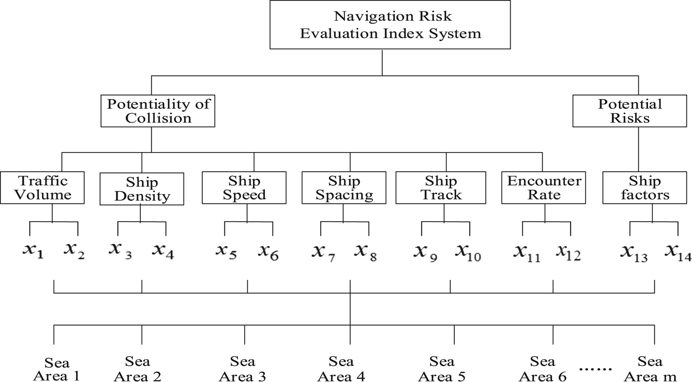
Figure 1. Configuration diagram of multi-objective and multi-layer system

In Figure 1, x ₁ is the average traffic volume; x ₂ is the peak traffic volume; x ₃ is the average ship density; x ₄ is the ship density distribution dispersion; x ₅ is the average ship speed; x ₆ is the ship speed distribution dispersion; x ₇ is the ship instantaneous spacing; x ₈ is the average ship spacing; x ₉ is the ship track overlap rate; x ₁₀ is the number of ship track intersection areas; x ₁₁ is the encounter rate based on DSPA; x ₁₂ is the encounter rate based on altering course collision avoidance; x ₁₃ is the ship type and x ₁₄ is the ship scale.

3.2. Multi-objective and Multi-layer Fuzzy Optimisation Model

In a system, there is a finite alternative (decision) set, consisting of n candidate alternatives (decisions):

(4)$$D=\lcub {d_1 ,d_2 ,\cdots ,d_n } \rcub $$

The first layer has t sets of juxtaposed unit systems, where the k-th unit system has the evaluation objective set which consists of the evaluations of m sets of objectives for the decision set D. The evaluation objective for the decision j is expressed as the vector:

(5)$${}_{1k}X_j =\lcub {{ }_{1k}x_{1j} ,{ }_{1k}x_{2j} ,\cdots {}_{1k}x_{mj}} \rcub $$

where _1kx _ij is the eigenvalue of the objective i for the j ^th decision in the first layer k-th unit system, i = 1, 2, 3, …, m, k = 1, 2, 3, …, t.

The objective eigenvalue matrix for n decisions in the first layer k-th unit system is expressed as:

(6)$${ }_{1k}X=\left[ \matrix{ \matrix{ {{ }_{1k}x_{11} } & {{ }_{1k}x_{12} } & \cdots & {{}_{1k}x_{1n} } \cr {{ }_{1k}x_{21} } & {{ }_{1k}x_{22} } & \cdots & {{ }_{1k}x_{2n} }} \cr {\cdots \cdots \cdots \cdots \cdots \cdots \cdots} \cr \matrix{ {{ }_{1k}x_{m1} } & {{ }_{1k}x_{m2} } & \cdots & {{}_{1k}x_{mn} }} } \right]={ }_{1k}(x_{ij} )$$

The objective eigenvalue matrix X is transformed to obtain the objective optimal relative membership matrix R:

(7)$${}_{1k}R=\left[ \matrix{ \matrix{ {{}_{1k}r_{11} } & {{}_{1k}r_{12} } & \cdots & {{}_{1k}r_{1n} } \cr {{}_{1k}r_{21} } & {{}_{1k}r_{22} } & \cdots & {{}_{1k}r_{2n} }} \cr {\cdots \cdots\cdots \cdots \cdots \cdots \cdots \cdots} \cr \matrix{ {{ }_{1k}r_{m1} } & {{}_{1k}r_{m2} } & \cdots & {{}_{1k}r_{mn} }}}\right]={}_{1k}(r_{ij})$$

where matrix X is transformed into matrix R by adopting the following objective optimal relative membership degree equation proposed by Chen (Reference Chen1994). Usually, there are two types of objectives, that is, profit and cost (Chen, Reference Chen, Fu, Wang and Liu2001), and their objective optimal relative membership degree can be expressed as follows:

In n alternatives (decisions), the value of objective i for a decision j is x _ij, where i = 1, 2, …, m and j = 1, 2, …, n.

In case of the profit type,

(8)$$r_{ij} ={x_{ij} -\mathop {\hbox{min}}\limits_j x_{ij} \over \mathop{\hbox{max}}\limits_j x_{ij} -\mathop {\hbox{min}}\limits_j x_{ij}}$$

(9)$$\hbox{Or}\, r_{ij} = {x_{ij} \over \mathop {\hbox{max}}\limits_j x_{ij} +\mathop{\hbox{min}}\limits_j x_{ij}}$$

In case of the cost type,

(10)$$r_{ij} ={\mathop {\hbox{max}}\limits_j x_{ij} - x_{ij} \over \mathop {\hbox{max}}\limits_j x_{ij} -\mathop {\hbox{min}}\limits_j x_{ij} }$$

(11)$$\hbox{Or}\, r_{ij} =1- {x_{ij} \over \mathop {\hbox{max}}\limits_j x_{ij} +\mathop {\hbox{min}}\limits_j x_{ij} }$$

where $\mathop {\max }\limits_{j} x_{ij}$ and $\mathop {\min }\limits_{j} x_{ij}$ are respectively the maximum and minimum eigenvalue of objective i in the decision set.

For the profit type, the larger the x _ij, the higher the objective optimal relative membership degree, the greater the risk to navigation. In Figure 1, x ₁, x ₂, x ₃, x ₄, x ₅, x ₆, x ₉, x ₁₀, x ₁₁, x ₁₂, x ₁₃ and x ₁₄ are profit objectives. For the cost type, the smaller the x _ij, the higher the objective optimal relative membership degree, the greater the risk to navigation. In Figure 1, x ₇ and x ₈ are cost objectives.

According to (Liu et al., Reference Liu, Wu and Jia2005b), when the variation range of the objective eigenvalue is large, Equations (8) and (10) are selected. When the variation range of the objective eigenvalue is small, Equations (9) and (11) are selected.

The first layer k-th unit system decision-making optimal relative membership degree model is:

(12)$${ }_{1k}u_j =1 \left/ {\left\{ {1+\left\{ {{\sum\limits_{i=1}^m {({ }_{1k}w_i (1-{ }_{1k}r_{ij} ))^p} \over \sum\limits_{i=1}^m {({ }_{1k}w_i { }_{1k}r_{ij} )^p} }} \right\}^{{2 \over p}}} \right\}}\right.$$

where p is the distance parameter: p = 1 (Hamming distance); p = 2 (Euclidean distance). The eigenvalue of m sets of objectives in the decision j have different weights, and the weight vector is:

(13)$${ }_{1k}w_j =({ }_{1k}w_{1j} ,{ }_{1k}w_{2j} ,\cdots ,{ }_{1k}w_{mj} ), \sum\limits_{i=1}^m {{ }_{1k}w_{ij} } =1$$

Assume that the optimal relative membership degree vector of the first layer k-th unit system is:

(14)$${} _{1k}u_j = ({}_{1k}u_1 ,{ }_{1k}u_{2,\ldots,} {}_{1k}u_n)$$

The optimal relative membership degree of all the unit systems in the first layer can be calculated by Equation (12), and the decision-making optimal relative membership degree matrix of the higher layer (second layer) is:

(15)$$U^{\ast }=\left[ \matrix{ \matrix{ {u_{11}^\ast } & {u_{12}^\ast } & \cdots & {u_{1n}^\ast } \cr {u_{21}^\ast } & {u_{22}^\ast } & \cdots & {u_{2n}^\ast }} \cr {\cdots \cdots \cdots \cdots \cdots \cdots } \cr \matrix{ {u_{t1}^\ast } & {u_{t2}^\ast } & \cdots & {u_{tn}^\ast } }} \right]=(u_{ij} ^\ast )$$

Let $u_{ij} ^{\ast} =r_{ij}^{\ast}$, w _ij* be the weight of the objectives in the unit systems of the higher layer, and $\sum\limits_{k=1}^{t} {w_{ij} ^{\ast}} =1$. According to the number of evaluation objectives, Equation (15) is calculated by using Equation (12) repeatedly. Therefore, from the low layer to high layer until the highest layer, the optimal relative membership degree vector can be obtained:

(16)$$u_j = (u_1 ,u_{2,\ldots ,} u_n )$$

The index weight vector is calculated as follows (Liu et al., Reference Liu, Wu and Jia2005a; Reference Liu, Wu and Jia2005b):

(17)$$w_i = {{\sum\limits_{j = 1}^n {r_{ij}} } \bigg{/} {\sum\limits_{i = 1}^m {\sum\limits_{j = 1}^n {r_{ij}} } }}$$

4.1. Target sea area and evaluation index eigenvalue

Through in-depth studies on the AIS-based data mining algorithm of real traffic, this paper has designed and developed an AIS-based statistical platform for ship traffic flow. The platform was developed in Microsoft Foundation Class Library (MFC) in Windows. It can statistically analyse the real traffic of sea areas over a specific period. In this paper, the coastal waters of Chengshantou were used as an example to illustrate the platform. According to the size of the waters, the Chengshantou waters was divided into 16 roughly similar-sized sea areas, marked as sea areas 1 to 16. The statistical platform display interface is shown in Figure 2.

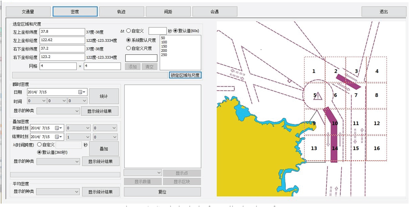
Figure 2. Statistical platform display interface.

Table 1 shows the evaluation index eigenvalue in each sea area.

Table 1. Raw traffic data based on AIS information.

4.2. Fuzzy Optimisation Decision-Making for Navigation Risk in Different Sea Areas

According to the data in Table 1, the eigenvalue matrix of target sea areas can be obtained as ${ }_{1k}X (k=1,2,3,4,5,6,7)$:

$$\eqalign{{ }_{11}X&=\left[ \matrix{ 8 & {12} & 9 & 6 & {21} & {10} & 5 & {13} & {12} & {25} & 3 & 4 & 2 & {23} & 3 & 5 \cr {12} & {15} & {13} & 8 & {27} & {14} & 8 & {17} & {16} & {30} & 6 & 8 & 4 & {28} & 5 & 8 \cr } \right]\cr { }_{12}X &=\left[ \matrix{ 7 & {11} & 8 & 5 & {19} & {11} & 4 & {10} \cr {1{\cdot}29} & {2{\cdot}21} & {2{\cdot}38} & {2{\cdot}94} & {2{\cdot}22} & {3{\cdot}15} & {2{\cdot}94} & {2{\cdot}44} \cr }\right.\cr &\left.\matrix{ &&9 & {20} & 2 & 4 & 2 & {15} & 2 & 3 \cr &&{2{\cdot}86} & {1{\cdot}84} & {2{\cdot}37} & {2{\cdot}55} & {3{\cdot}09} & {1{\cdot}77} & {2{\cdot}09} & {3{\cdot}51} \cr }\right]\cr { }_{13}X &=\left[ \matrix{ {10{\cdot}3} & {12{\cdot}5} & {12{\cdot}2} & {13{\cdot}2} & {10{\cdot}5} & {10{\cdot}8} & {11{\cdot}8} & {10{\cdot}8} \cr {2{\cdot}44} & {3{\cdot}83} & {3{\cdot}73} & {3{\cdot}46} & {2{\cdot}24} & {1{\cdot}67} & {3{\cdot}38} & {3{\cdot}74} \cr }\right.\cr &\left.\matrix{ && {9{\cdot}4} & {10{\cdot}8} & {11{\cdot}9} & {12{\cdot}1} & {8{\cdot}1} & {9{\cdot}7} & {7{\cdot}5} & {11{\cdot}3} \cr && {3{\cdot}39} & {3{\cdot}26} & {5{\cdot}61} & {4{\cdot}77} & {6{\cdot}60} & {3{\cdot}16} & {6{\cdot}32} & {2{\cdot}97} \cr }\right]\cr { }_{14}X&=\left[ \matrix{ {2{\cdot}54} & {1{\cdot}25} & {1{\cdot}17} & {1{\cdot}98} & {0{\cdot}78} & {1{\cdot}39} & {1{\cdot}52} & {2{\cdot}51} \cr {2{\cdot}24} & {1{\cdot}34} & {1{\cdot}08} & {2{\cdot}21} & {0{\cdot}89} & {1{\cdot}01} & {1{\cdot}23} & {2{\cdot}43} \cr }\right.\cr &\left.\matrix{ && {0{\cdot}92} & {1{\cdot}95} & {1{\cdot}82} & {2{\cdot}61} & {1{\cdot}28} & {0{\cdot}82} & {1{\cdot}78} & {1{\cdot}32} \cr && {1{\cdot}05} & {1{\cdot}61} & {2{\cdot}01} & {2{\cdot}09} & {2{\cdot}03} & {0{\cdot}79} & {2{\cdot}08} & {1{\cdot}98} \cr }\right]\cr { }_{15}X &=\left[ \matrix{ {29{\cdot}6} & {18{\cdot}5} & {15{\cdot}7} & {14{\cdot}3} & {32{\cdot}4} & {39{\cdot}0} & {15{\cdot}2} & {9{\cdot}1} \cr 2 & 2 & 4 & 1 & 4 & 3 & 3 & 2 \cr }\right.\cr &\left.\matrix{ && {11{\cdot}2} & {23{\cdot}0} & {18{\cdot}5} & {6{\cdot}7} & {7{\cdot}8} & {10{\cdot}0} & {8{\cdot}5} & {5{\cdot}2}\cr && 3 & 1 & 2 & 1 & 2 & 1 & 2 & 3 \cr }\right]\cr { }_{16}X &=\left[ \matrix{ 8 & 6 & {13} & 5 & {17} & {11} & {10} & 5 & {15} & 7 & 6 & 3 & 5 & 9 & 4 & 3 \cr 6 & 9 & {10} & 4 & {15} & {13} & 8 & 7 & {10} & 9 & 4 & 5 & 4 & 7 & 6 & 5 \cr } \right]\cr { }_{17}X &=\left[ \matrix{ {7{\cdot}5} & {20} & {21} & {4{\cdot}5} & {18} & {13} & 7 & 4 \cr {12{\cdot}5} & {10} & {9{\cdot}5} & 5 & {15} & {19} & {13} & 5 \cr }\right.\cr &\left.\matrix{ && {10{\cdot}5} & {11} & 5 & {4{\cdot}5} & {1{\cdot}5} & {11{\cdot}8} & {3{\cdot}7} & 4 \cr && {7{\cdot}6} & {8{\cdot}1} & 3 & {1{\cdot}8} & {3{\cdot}4} & {0{\cdot}5} & 4 & 5 \cr } \right]}$$

x ₇ and x ₈ are the cost types; others are the profit types. Since the variation of the objective eigenvalue is small, Equations (9) and (11) are selected. The optimal relative membership degree matrix of the first layer can be obtained as ${ }_{1k}u (k=1,2,3,4,5,6,7)$:

$$\eqalign{{ }_{11}u&=\left[ \matrix{ {0{\cdot}296} & {0{\cdot}444} & {0{\cdot}333} & {0{\cdot}222} & {0{\cdot}777} & {0{\cdot}370} & {0{\cdot}185} & {0{\cdot}481}\cr 0{\cdot}352 & 0{\cdot}441 & 0{\cdot}382 & 0{\cdot}235 & 0{\cdot}794 & 0{\cdot}411 & 0{\cdot}233 & 0{\cdot}500\cr } \right.\cr &\left.\matrix{ & & {0{\cdot}444} & {0{\cdot}925} & {0{\cdot}111} & {0{\cdot}148} & {0{\cdot}074} & {0{\cdot}851} & {0{\cdot}111} & {0{\cdot}185} \cr & & 0{\cdot}470 & 0{\cdot}882 & 0{\cdot}176 & 0{\cdot}235 & 0{\cdot}117 & 0{\cdot}823 & 0{\cdot}147 & 0{\cdot}235 \cr } \right]\cr { }_{12}u&=\left[ \matrix{ 0{\cdot}318 & 0{\cdot}500 & 0{\cdot}363 & 0{\cdot}227 & 0{\cdot}863 & 0{\cdot}500 & 0{\cdot}181 & 0{\cdot}454 \cr 0{\cdot}268 & 0{\cdot}460 & 0{\cdot}495 & 0{\cdot}612 & 0{\cdot}462 & 0{\cdot}656 & 0{\cdot}612 & 0{\cdot}508 \cr } \right.\cr &\left.\matrix{ && 0{\cdot}409 & 0{\cdot}909 & 0{\cdot}090 & 0{\cdot}181 & 0{\cdot}090 & 0{\cdot}681 & 0{\cdot}090 & 0{\cdot}136 \cr && 0{\cdot}595 & 0{\cdot}383 & 0{\cdot}493 & 0{\cdot}531 & 0{\cdot}643 & 0{\cdot}368 & 0{\cdot}435 & 0{\cdot}731 \cr } \right] \cr { }_{13}u&=\left[ \matrix{ 0{\cdot}497 & 0{\cdot}603 & 0{\cdot}589 & 0{\cdot}637 & 0{\cdot}507 & 0{\cdot}521 & 0{\cdot}570 & 0{\cdot}521 \cr 0{\cdot}295 & 0{\cdot}463 & 0{\cdot}451 & 0{\cdot}418 & 0{\cdot}270 & 0{\cdot}201 & 0{\cdot}408 & 0{\cdot}452 \cr } \right.\cr &\left.\matrix{ && 0{\cdot}454 & 0{\cdot}521 & 0{\cdot}574 & 0{\cdot}584 & 0{\cdot}391 & 0{\cdot}468 & 0{\cdot}362 & 0{\cdot}545 \cr && 0{\cdot}409 & 0{\cdot}394 & 0{\cdot}678 & 0{\cdot}576 & 0{\cdot}798 & 0{\cdot}382 & 0{\cdot}764 & 0{\cdot}359 \cr } \right]\cr { }_{14}u&=\left[ \matrix{ 0{\cdot}250 & 0{\cdot}631 & 0{\cdot}654 & 0{\cdot}415 & 0{\cdot}769 & 0{\cdot}590 & 0{\cdot}551 & 0{\cdot}259\cr 0{\cdot}304 & 0{\cdot}583 & 0{\cdot}664 & 0{\cdot}313 & 0{\cdot}723 & 0{\cdot}686 & 0{\cdot}618 & 0{\cdot}245 \cr } \right.\cr &\left.\matrix{ && 0{\cdot}728 & 0{\cdot}424 & 0{\cdot}463 & 0{\cdot}230 & 0{\cdot}622 & 0{\cdot}758 & 0{\cdot}474 & 0{\cdot}315 \cr && 0{\cdot}673 & 0{\cdot}500 & 0{\cdot}375 & 0{\cdot}350 & 0{\cdot}369 & 0{\cdot}754 & 0{\cdot}354 & 0{\cdot}385 \cr } \right] \cr { }_{15}u&=\left[ \matrix{ 0{\cdot}669 & 0{\cdot}418 & 0{\cdot}355 & 0{\cdot}323 & 0{\cdot}733 & 0{\cdot}882 & 0{\cdot}343 & 0{\cdot}205 \cr 0{\cdot}400 & 0{\cdot}400 & 0{\cdot}800 & 0{\cdot}200 & 0{\cdot}800 & 0{\cdot}600 & 0{\cdot}600 & 0{\cdot}400 \cr } \right.\cr &\left.\matrix{ && 0{\cdot}253 & 0{\cdot}520 & 0{\cdot}418 & 0{\cdot}151 & 0{\cdot}176 & 0{\cdot}226 & 0{\cdot}192 & 0{\cdot}117 \cr && 0{\cdot}600 & 0{\cdot}200 & 0{\cdot}400 & 0{\cdot}200 & 0{\cdot}400 & 0{\cdot}200 & 0{\cdot}400 & 0{\cdot}600 \cr } \right]\cr { }_{16}u&=\left[ \matrix{ 0{\cdot}400 & 0{\cdot}300 & 0{\cdot}650 & 0{\cdot}250 & 0{\cdot}850 & 0{\cdot}550 & 0{\cdot}500 & 0{\cdot}250 \cr 0{\cdot}315 & 0{\cdot}473 & 0{\cdot}526 & 0{\cdot}210 & 0{\cdot}789 & 0{\cdot}684 & 0{\cdot}421 & 0{\cdot}368 \cr } \right.\cr &\left.\matrix{ && 0{\cdot}750 & 0{\cdot}350 & 0{\cdot}300 & 0{\cdot}150 & 0{\cdot}250 & 0{\cdot}450 & 0{\cdot}200 & 0{\cdot}150 \cr && 0{\cdot}526 & 0{\cdot}473 & 0{\cdot}210 & 0{\cdot}263 & 0{\cdot}210 & 0{\cdot}368 & 0{\cdot}315 & 0{\cdot}263 \cr } \right]\cr { }_{17}u&=\left[ \matrix{ 0{\cdot}333 & 0{\cdot}888 & 0{\cdot}933 & 0{\cdot}200 & 0{\cdot}800 & 0{\cdot}577 & 0{\cdot}311 & 0{\cdot}177 \cr 0{\cdot}641 & 0{\cdot}512 & 0{\cdot}487 & 0{\cdot}256 & 0{\cdot}769 & 0{\cdot}974 & 0{\cdot}666 & 0{\cdot}256 \cr } \right.\cr &\left.\matrix{ && 0{\cdot}466 & 0{\cdot}488 & 0{\cdot}222 & 0{\cdot}200 & 0{\cdot}066 & 0{\cdot}524 & 0{\cdot}164 & 0{\cdot}177 \cr && 0{\cdot}389 & 0{\cdot}415 & 0{\cdot}153 & 0{\cdot}092 & 0{\cdot}174 & 0{\cdot}025 & 0{\cdot}205 & 0{\cdot}256 \cr } \right]}$$

The first layer weight vector is calculated according to Equation (17):

$$\eqalign{{ }_{11}w &= (0\cdot4807, 0\cdot5193) \quad { }_{12}w= (0\cdot4207, 0\cdot5793) \quad{ }_{13}w= (0\cdot5328, 0\cdot4672)\cr { }_{14}w &= (0\cdot5074, 0\cdot4926) \quad{ }_{15}w= (0\cdot4541, 0\cdot5459) \quad{ }_{16}w= (0\cdot4972, 0\cdot5028)\cr { }_{17}w &= (0\cdot5100, 0\cdot4900)}$$

According to Equation (12), the optimal relative membership degree matrix of the second layer can be obtained:

$$\eqalign{{ }_2u&=\left[ \matrix{ 0{\cdot}191 & 0{\cdot}386 & 0{\cdot}240 & 0{\cdot}081 & 0{\cdot}931 & 0{\cdot}295 & 0{\cdot}068 & 0{\cdot}482 \cr 0{\cdot}138 & 0{\cdot}448 & 0{\cdot}402 & 0{\cdot}463 & 0{\cdot}670 & 0{\cdot}692 & 0{\cdot}432 & 0{\cdot}479 \cr 0{\cdot}331 & 0{\cdot}581 & 0{\cdot}557 & 0{\cdot}580 & 0{\cdot}325 & 0{\cdot}297 & 0{\cdot}498 & 0{\cdot}483 \cr 0{\cdot}128 & 0{\cdot}764 & 0{\cdot}789 & 0{\cdot}252 & 0{\cdot}896 & 0{\cdot}752 & 0{\cdot}662 & 0{\cdot}102 \cr 0{\cdot}519 & 0{\cdot}321 & 0{\cdot}689 & 0{\cdot}105 & 0{\cdot}918 & 0{\cdot}841 & 0{\cdot}491 & 0{\cdot}192 \cr 0{\cdot}238 & 0{\cdot}292 & 0{\cdot}667 & 0{\cdot}082 & 0{\cdot}952 & 0{\cdot}719 & 0{\cdot}421 & 0{\cdot}171 \cr 0{\cdot}465 & 0{\cdot}817 & 0{\cdot}815 & 0{\cdot}080 & 0{\cdot}930 & 0{\cdot}871 & 0{\cdot}467 & 0{\cdot}072 \cr } \right.\cr &\left.\matrix{ && 0{\cdot}417 & 0{\cdot}987 & 0{\cdot}029 & 0{\cdot}057 & 0{\cdot}012 & 0{\cdot}963 & 0{\cdot}022 & 0{\cdot}068\cr && 0{\cdot}560 & 0{\cdot}602 & 0{\cdot}263 & 0{\cdot}343 & 0{\cdot}426 & 0{\cdot}457 & 0{\cdot}204 & 0{\cdot}539\cr && 0{\cdot}372 & 0{\cdot}434 & 0{\cdot}724 & 0{\cdot}658 & 0{\cdot}615 & 0{\cdot}365 & 0{\cdot}563 & 0{\cdot}432\cr && 0{\cdot}846 & 0{\cdot}423 & 0{\cdot}346 & 0{\cdot}145 & 0{\cdot}499 & 0{\cdot}906 & 0{\cdot}339 & 0{\cdot}225\cr && 0{\cdot}425 & 0{\cdot}221 & 0{\cdot}321 & 0{\cdot}046 & 0{\cdot}179 & 0{\cdot}066 & 0{\cdot}186 & 0{\cdot}346\cr && 0{\cdot}743 & 0{\cdot}332 & 0{\cdot}107 & 0{\cdot}068 & 0{\cdot}082 & 0{\cdot}324 & 0{\cdot}112 & 0{\cdot}068\cr && 0{\cdot}363 & 0{\cdot}408 & 0{\cdot}053 & 0{\cdot}033 & 0{\cdot}021 & 0{\cdot}200 & 0{\cdot}048 & 0{\cdot}072\cr } \right]}$$

Similarly, the second layer weight vector is obtained from Equation (17):

$${ }_2w=(0{\cdot}1159,0{\cdot}1578,0{\cdot}1731,0{\cdot}1776,0{\cdot}1299,0{\cdot}1191,0{\cdot}1226)$$

The optimal relative membership degree vector of navigation risk in multi-objective and multi-layer high-risk sea areas are obtained by Equation (12):

$$\eqalign{u_j &= ({0{\cdot}143,0{\cdot}564},{0{\cdot}680},{0{\cdot}182,0{\cdot}844},{0{\cdot}702},0{\cdot}450,0{\cdot}181,0{\cdot}588,0{\cdot}454, \cr &\quad 0{\cdot}235,0{\cdot}154, 0{\cdot}252,0{\cdot}493,0{\cdot}150,0{\cdot}174)}$$

According to the principle that the higher the optimal relative membership degree, the greater the navigation risk, the 16 sea areas can be ranked from high risk to low risk as follows: sea area 5, 6, 3, 9, 2, 14, 10, 7, 13, 11, 4, 8, 16, 12, 15, 1. Among them, the risk degree of sea areas 5, 6 and 3 is higher, and the risk degree of sea areas 12, 15 and 1 is lower.

5.1. The verification from the perspective of real traffic

Since 1 June 2015, a new Traffic Separation Scheme (TSS) has been implemented in the waters of Chengshantou. On the eastern side of the original TSS, a new Outer Traffic Separation Scheme (OTSS) was added as shown in Figure 2, including the Outer Traffic Separation Lanes (OTSL) and the outer precautionary area. The OTSL are composed of the east, north and south traffic separation lanes and the separation zone. In the 16 sea areas of Chengshantou waters, sea areas 11, 12, 15 and 16 mainly include part of south traffic separation lane of the OTSL. Sea areas 3, 4, 7 and 8 mainly include parts of east, south and north traffic separation lanes of the OTSL and part of the outer precautionary area. Sea areas 1, 2, 5 and 6 mainly include the inner precautionary area, part of the outer precautionary areas and part of the north traffic separation lane of the OTSL. Sea areas 9, 10, 13 and 14 mainly include the south traffic separation lane of the original inner traffic separation lanes.

All ships entering and exiting Bohai Bay using the OTSS need to sail through sea areas 5, 6 and part of sea area 2. They encounter at the inner and outer precautionary area, where the ship traffic volume is large, the average ship spacing is small, collision avoidance manoeuvring is frequent and the encounter rate is high. Therefore, the collision risk is higher in these sea areas. The vessels sailing through sea areas 3 and 7 using the OTSS include ships sailing northward to Dalian Port and other ports in the north, some ships entering and exiting the Bohai Bay, ships sailing eastward to Japan and South Korea and ships sailing southward. In this area, the ship traffic volume, the angle of altering course and the ship scale are large, the ship manoeuvring is difficult, and the potential risk to safety of navigation is relatively higher. Sea areas 9 and 13 are close to the coast. There are many fishing boats in this area, resulting in smaller ship spacing and higher collision risk. The ship traffic volume in sea areas 10 and 14 is very large, resulting in an increase in the ship density. The proportion of some dangerous goods ships and large ships also rises in these areas which leads to higher collision risk. Although the tonnage of ships sailing in sea areas 11 and 12 is large, ships do not need to alter their courses. Since the encounter rate is low in these areas, the collision risk is low.

Using the platform, the 72-hour ship track distribution and the 12-hour overlapped graph of ship density in Chengshantou waters are shown in Figure 3. Figure 3(a) is the display of 72-hour track distribution according to course. Figure 3(b) is the display of 72-hour track distribution according to ship scale. Figure 3(c) is the display of 72-hour track according to ship type. Figure 3(d) is the 12-hour overlapped graph of ship density. From Figure 3, it can be observed that the 72-hour ship track distribution and the 12-hour ship density situation in Chengshantou waters is consistent with the above analysis of the traffic flow in 16 sea areas. In addition, the navigation risk analysis in the 16 sea areas is consistent with the decision model calculation results. Therefore, the model can be shown to be scientific and practical.

Figure 3. Display of 72-hour ship track distribution and 12-hour ship density in Chengshanjiao waters.

5.2. The verification from the perspective of fuzzy comprehensive evaluation model results

To further verify the results of the decision model, a fuzzy comprehensive evaluation model of the safety evaluation was selected, and the weight of each index was determined based on the improved Analytic Hierarchy Process (AHP), i.e., Fuzzy Analytic Hierarchy Process (FAHP). Following the advice of experts such as Zhaolin Wu, Dexin Liu and Yuhui Fu from Dalian Maritime University, the evaluation criteria of each index were determined and the corresponding membership functions were established. Finally, the fuzzy comprehensive evaluation was applied to the 16 sea areas one by one to determine their navigation risk. Among them, the evaluation level of the evaluation set is defined as:

(18)$$V=\lcub {v_1 ,v_2 ,v_3 ,v_4 ,v_5 } \rcub $$

where v ₁ ~ v ₅ represents the rating of the evaluation: very low risk, low risk, general risk, high risk, very high risk. Their corresponding fuzzy numbers are 1, 2, 3, 4 and 5.

Through the calculation, the membership degree of each sea area and the comprehensive evaluation results based on a weighted average are shown in Table 2.

Table 2. Fuzzy comprehensive evaluation results.

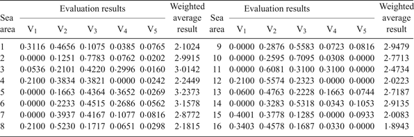
According to the principle that the larger the weighted average result, the higher the risk, the 16 sea areas can be ranked from high risk to low risk as follows: sea areas 5, 6, 3, 2, 9, 14, 7, 10, 13, 11, 4, 8, 1, 12, 15, 16. Comparing this ranking with the evaluation from the multi-objective and multi-layer fuzzy optimisation decision model (from high risk to low risk: sea area 5, 6, 3, 9, 2, 14, 10, 7, 13, 11, 4, 8, 16, 12, 15, 1), it can be found that the results of the two models are similar, although the sorting is different in some parts. This is mainly due to different weighting methods of the two model indices. The index weight of the decision model is objective, while the index weight of the fuzzy comprehensive evaluation model is subjective with preference for certain indices. However, the differences are so small that it can be accepted. Therefore, it can be concluded that the objective evaluation of the decision model is consistent with people's subjective understanding, which further validates the rationality and feasibility of the multi-objective and multi-layer fuzzy optimisation model.