1 Introduction
When a solid particle comes into contact with another particle or solid surface, it exchanges electric charge. This phenomenon is commonly referred to as triboelectric charging and is encountered in many different settings. Examples in nature include the formation of lasting geological patterns under arid conditions such as razorbacks observed on Mars (Shinbrot, LaMarche & Glasser Reference Shinbrot, LaMarche and Glasser2006). Strong electrostatic charging has also been observed during volcanic eruptions (Miura, Koyaguchi & Tanaka Reference Miura, Koyaguchi and Tanaka2002) as well as during aeolian transport of grains (Kamra Reference Kamra1972).
In an industrial context, this phenomenon is used in electrostatic separation of different kinds of insulating materials (Laurentie, Traoré & Dascalescu Reference Laurentie, Traoré and Dascalescu2013), in electrophotography (Schein Reference Schein1999) and in various other applications. Moreover, it is responsible for the electrification of powder that is often observed during pneumatic conveying processes (Matsusaka et al. Reference Matsusaka, Maruyama, Matsuyama and Ghadiri2010). Due to its far-reaching effects, both beneficial and unfavourable, the phenomenon of tribolectric charging has attracted considerable attention over the years. Experimental studies, such as those of Masuda, Komatsu & Iinoya (Reference Masuda, Komatsu and Iinoya1976), Artana, Touchard & Morin (Reference Artana, Touchard and Morin1997), Tanoue et al. (Reference Tanoue, Tanaka, Kitano and Masuda2001), Nifuku & Katoh (Reference Nifuku and Katoh2003), Nomura, Satoh & Masuda (Reference Nomura, Satoh and Masuda2003), Watano, Saito & Suzuki (Reference Watano, Saito and Suzuki2003), Watano (Reference Watano2006) and Fath et al. (Reference Fath, Blum, Glor and Walther2013), explored the influence of various parameters on the charging of powder, including conveying air velocity, powder mass loading, material properties of the powder and ambient air humidity. However, the results of the above experimental studies are not conclusive because the measurements either exhibit large scatter or they do not agree with each other, which does not allow for a full understanding of the electrification process. This inconclusiveness may be attributed to several factors that are not fully controllable in an experiment, most notably: (i) the exact physical mechanism of charge transfer, (ii) the initial and boundary conditions for the particulate phase and (iii) the emerging flow patterns.
As regards the first factor, i.e. the physical mechanism of charge transfer, it was elaborated in the review paper of Matsusaka et al. (Reference Matsusaka, Maruyama, Matsuyama and Ghadiri2010) and in the more recent one of Wong, Kwok & Chan (Reference Wong, Kwok and Chan2015) that there is still no consensus as to which species is mainly responsible for the charge transfer. While most researchers assume transfer of electrons (Harper Reference Harper1951; Murata & Kittaka Reference Murata and Kittaka1979; Shirakawa et al. Reference Shirakawa, Ii, Yoshida, Takashima, Shimosaka and Hidaka2008), others relate it to the transfer of ions (Robins, Lowell & Rose-Innes Reference Robins, Lowell and Rose-Innes1980; Diaz & Fenzel-Alexander Reference Diaz and Fenzel-Alexander1993). Further, it was claimed that, during contact, patches of bulk material in the micrometre or nanometre scale are torn off and deposited onto the other surface (Lowell & Rose-Innes Reference Lowell and Rose-Innes1980; Tanoue, Ema & Masuda Reference Tanoue, Ema and Masuda1999; Lacks Reference Lacks2012). The exact type of transferred species might even vary spatially and temporally (Baytekin et al. Reference Baytekin, Patashisnki, Branicki, Baytekin, Soh and Grzybowski2011).
The influence of the second factor, i.e. the initial and boundary conditions, was elucidated by the experimental investigations of Masui & Murata (Reference Masui and Murata1983) and Yamamoto & Scarlett (Reference Yamamoto and Scarlett1986) who shot single particles at a target and measured their charge before and after the impact. They reported that the charge exchange depends strongly on the initial charges that are carried by the particles. In a similar experimental set-up, Matsuyama et al. (Reference Matsuyama, Ogu, Yamamoto, Marijnissen and Scarlett2003) demonstrated that the charge exchange depends not only on the value of the initial charge but also on its local distribution on the particles surface. This finding was subsequently taken into account in the theoretical considerations of Grosshans & Papalexandris (Reference Grosshans and Papalexandris2016c ) who proposed a model for contact charging that takes into account the non-uniformities of charge distribution on a particle surface. It is also worth mentioning that when a powder is brought into an experimental facility, the handling of the powder results in an electric charging that is very difficult to estimate and that, more often than not, is not taken into account. This partially explains the large scatter observed in experimental measurements.
Further, the dynamics of particles in a pipe flow depends on the inlet boundary conditions and the manner with which particles are introduced to the test section. For example, Tsuji, Morikawa & Shiomi (Reference Tsuji, Morikawa and Shiomi1984) investigated the flow patters of non-charging solid–fluid mixtures in pipes and reported that the particles were sliding, due to centrifugal forces, on the outer wall of a bend shortly before entering the test section. In these experiments, a 5110 mm long pipe was used so as to ensure that the particle motion has reached steady state. The charging of the particles up to this point is affected by the inlet boundary conditions which further contributes to the scatter of experimental results.
With respect to the third factor, i.e. the emerging flow patterns, the strong coupling between fluid dynamics, particle dynamics and electrostatics was evidenced by Schmid & Vogel (Reference Schmid and Vogel2003). Finally, deviations of the particle shape from sphericity can lead to significant changes in its charging behaviour, as pointed out by Ireland (Reference Ireland2012).
The uncertainties involved in the prescription of initial and boundary conditions during experiments provided motivation for numerical studies of triboelectric charging. Most of them concerned full-scale simulations of flows in circular pipes. The drawback of full-scale studies is that, due to the large size of the flow domain, they are computationally very expensive. Consequently, quite often the dynamics of the flow had to be represented in a rather simplified manner. For example, in their numerical studies, Watano et al. (Reference Watano, Saito and Suzuki2003) assumed a pre-defined velocity profile for the carrier fluid. A more realistic approach was followed by Kolniak & Kuczynski (Reference Kolniak and Kuczynski1989) and Tanoue et al. (Reference Tanoue, Ema and Masuda1999, Reference Tanoue, Tanaka, Kitano and Masuda2001) who performed simulations of triboelectric charging based on the Reynolds-averaged Navier–Stokes (RANS) approach. Whereas the predictions of RANS simulations can be sensitive to the choice of turbulence model, large eddy simulations (LES) such as those performed, for example, by Lim, Yao & Zhao (Reference Lim, Yao and Zhao2012), Korevaar et al. (Reference Korevaar, Padding, Van der Hoef and Kuipers2014), Grosshans & Papalexandris (Reference Grosshans and Papalexandris2016a ,Reference Grosshans and Papalexandris b ) and Grosshans, Szasz & Papalexandris (Reference Grosshans, Szasz and Papalexandris2017) provided more accurate estimations of the charging of powders. These numerical studies confirmed the strong dependence of powder charging on the Reynolds number of the flow, mass flow rate of the powder and on the pipe diameter. However, LES are not free of uncertainties and potential sources of errors either, especially as regards the prediction of charge exchange in the near-wall regions.
These uncertainties and errors can be mitigated in direct numerical simulations (DNS). However, and to the best of our knowledge, DNS of tribolectric charging are currently not available in the literature. Nonetheless, over the years DNS has become a computationally affordable and, therefore, increasingly popular approach for the study of particle-laden flows. For example, McLaughlin (Reference McLaughlin1989) performed DNS of a vertical channel flow in which rigid spherical particles were released. In that study, the author reported that particles tend to accumulate in the viscous sublayer, i.e. within the first five wall units. This was explained by inward turbulent motions in the buffer region, the so-called sweeps. The phenomenon is known as turbophoresis and had been observed previously in various different settings (Caporaloni et al. Reference Caporaloni, Tampieri, Trombetti and Vittori1975; Reeks Reference Reeks1983). It is typically described as a process of two phases that have different time scales. In the first phase, particles are driven away from the centreplane of the channel toward the wall by energetic turbulent convection. In the second phase, they are transported slowly by small-scale turbulent structures.
Marchioli & Soldati (Reference Marchioli and Soldati2002) also performed DNS of particle-laden channel flows and investigated the coherent structures that give rise to non-uniform particle distribution profiles. They were able to identify the characteristic patterns which are responsible for particle trapping close to the wall. More recent DNS studies on this field include the one by Wang (Reference Wang2010) who investigated the preferential location and turbulence modulation by particles of different inertia and volumetric concentrations. Further, Milici et al. (Reference Milici, De Marchis, Sardina and Napoli2014) and De Marchis et al. (Reference De Marchis, Milici, Sardina and Napoli2016) elucidated the influence of the wall roughness on the particle dynamics and flow characteristics.
In this paper we report on DNS of triboelectric charging in particle-laden channel flows at moderate turbulent intensities. The motivation of our study is to gain a better understanding of the build-up of particle charge in turbulent flows and to provide a deeper insight on the underlying physical mechanisms. Of particular interest is the elucidation of the effect of turbophoresis, particularly since particle electrification takes place during wall collisions, i.e. close to the region where particles agglomerate due to turbophoretic drift. In fact, the interplay between these two mechanisms has not been studied before. The effects of certain important parameters, such as the Stokes number, are also investigated and described herein.
Our paper is structured as follows. In § 2 we present an outline of the hydrodynamics and electrostatics model. In § 3 we describe the numerical set-up for our simulations. Section 4 contains the presentation and discussion of our numerical results and parametric studies. Finally, § 5 concludes.
2 Mathematical modelling
2.1 Hydrodynamics model
Let us consider a mixture consisting of a simple Newtonian carrier fluid and
 $N$
particles. The flow of the carrier fluid is assumed to be incompressible and is described in an Eulerian framework by the Navier–Stokes equations with constant diffusivity. The flow is considered to be dilute, i.e. the volume occupied by the particulate phase is very small compared to the volume occupied by the fluid. Further, four-way coupling is taken into account by introducing appropriate source terms to the evolution equations for both phases (Elgobashi Reference Elgobashi1994). The suitability of this approach to treat dilute solid–fluid mixtures was discussed in detail by Toschi & Bodenschatz (Reference Toschi and Bodenschatz2009) and Balachandar & Eaton (Reference Balachandar and Eaton2010). Accordingly, the mass and momentum balance laws for the fluid phase read
$N$
particles. The flow of the carrier fluid is assumed to be incompressible and is described in an Eulerian framework by the Navier–Stokes equations with constant diffusivity. The flow is considered to be dilute, i.e. the volume occupied by the particulate phase is very small compared to the volume occupied by the fluid. Further, four-way coupling is taken into account by introducing appropriate source terms to the evolution equations for both phases (Elgobashi Reference Elgobashi1994). The suitability of this approach to treat dilute solid–fluid mixtures was discussed in detail by Toschi & Bodenschatz (Reference Toschi and Bodenschatz2009) and Balachandar & Eaton (Reference Balachandar and Eaton2010). Accordingly, the mass and momentum balance laws for the fluid phase read
 $$\begin{eqnarray}\displaystyle & \unicode[STIX]{x1D735}\boldsymbol{\cdot }\boldsymbol{u}=0, & \displaystyle\end{eqnarray}$$
 $$\begin{eqnarray}\displaystyle & \displaystyle \frac{\unicode[STIX]{x2202}\boldsymbol{u}}{\unicode[STIX]{x2202}t}+(\boldsymbol{u}\boldsymbol{\cdot }\unicode[STIX]{x1D735})\boldsymbol{u}=-\frac{1}{\unicode[STIX]{x1D70C}}\unicode[STIX]{x1D735}p+\unicode[STIX]{x1D708}\unicode[STIX]{x1D6FB}^{2}\boldsymbol{u}+\boldsymbol{F}_{s}. & \displaystyle\end{eqnarray}$$
In the above equations
 $\boldsymbol{u}=(u,v,w)$
stands for the fluid velocity vector, and
$\boldsymbol{u}=(u,v,w)$
stands for the fluid velocity vector, and
 $p$
,
$p$
,
 $\unicode[STIX]{x1D70C}$
and
$\unicode[STIX]{x1D70C}$
and
 $\unicode[STIX]{x1D708}$
represent the fluid pressure, density and kinematic viscosity, respectively. The source term
$\unicode[STIX]{x1D708}$
represent the fluid pressure, density and kinematic viscosity, respectively. The source term
 $\boldsymbol{F}_{s}$
accounts for the momentum transfer between the particles and the carrier fluid. More specifically, its integral over a control volume is equal to the opposite of the sum of the aerodynamic drag forces that act on the particles that are located inside the control volume.
$\boldsymbol{F}_{s}$
accounts for the momentum transfer between the particles and the carrier fluid. More specifically, its integral over a control volume is equal to the opposite of the sum of the aerodynamic drag forces that act on the particles that are located inside the control volume.
The convective terms are approximated via a weighted essentially non-oscillatory upwind scheme that is up to fifth-order accurate (Jang & Shu Reference Jang and Shu1996), whereas the diffusive and pressure terms are approximated via fourth-order central differences. Finally, time integration is performed by an implicit second-order backward scheme. The reader is referred to Gullbrand, Bai & Fuchs (Reference Gullbrand, Bai and Fuchs2001) for further details concerning the numerical implementation.
As regards the particulate phase, we assume that it is the ensemble of
 $N$
spherical and rigid particles. Let
$N$
spherical and rigid particles. Let
 $\unicode[STIX]{x1D70C}_{p}$
,
$\unicode[STIX]{x1D70C}_{p}$
,
 $r_{p}$
and
$r_{p}$
and
 $m_{p}=(4/3)\unicode[STIX]{x03C0}\unicode[STIX]{x1D70C}_{p}r_{p}^{3}$
be the material density, radius and mass of a single particle, respectively. The particles are assumed to be made of the same material and, therefore, their material densities are equal. For computational purpose, each particle is treated individually as a point mass whose motion is computed in a Lagrangian framework. Then, the acceleration of a single particle is given by
$m_{p}=(4/3)\unicode[STIX]{x03C0}\unicode[STIX]{x1D70C}_{p}r_{p}^{3}$
be the material density, radius and mass of a single particle, respectively. The particles are assumed to be made of the same material and, therefore, their material densities are equal. For computational purpose, each particle is treated individually as a point mass whose motion is computed in a Lagrangian framework. Then, the acceleration of a single particle is given by
 $$\begin{eqnarray}\frac{\text{d}\boldsymbol{u}_{p}}{\text{d}t}=\boldsymbol{f}_{ad}+\boldsymbol{f}_{el}+\boldsymbol{f}_{coll}+\boldsymbol{f}_{g},\end{eqnarray}$$
where
 $\boldsymbol{u}_{p}$
is the velocity of the given particle and
$\boldsymbol{u}_{p}$
is the velocity of the given particle and
 $\boldsymbol{f}_{ad}$
,
$\boldsymbol{f}_{ad}$
,
 $\boldsymbol{f}_{el}$
,
$\boldsymbol{f}_{el}$
,
 $\boldsymbol{f}_{coll}$
and
$\boldsymbol{f}_{coll}$
and
 $\boldsymbol{f}_{g}$
denote, respectively, the acceleration due to the aerodynamic drag, electric field, collisional and gravitational forces acting on the particle.
$\boldsymbol{f}_{g}$
denote, respectively, the acceleration due to the aerodynamic drag, electric field, collisional and gravitational forces acting on the particle.
The acceleration due to the net effect of gravity on the particle reads
 $$\begin{eqnarray}\boldsymbol{f}_{g}=\left(1-{\displaystyle \frac{\unicode[STIX]{x1D70C}}{\unicode[STIX]{x1D70C}_{p}}}\right)\boldsymbol{g},\end{eqnarray}$$
where
 $\boldsymbol{g}$
is the gravitational acceleration.
$\boldsymbol{g}$
is the gravitational acceleration.
The collisional acceleration term
 $\boldsymbol{f}_{coll}$
accounts for both inter-particle and particle–wall collisions. In the present work we consider fully elastic and binary particle–particle collisions. In order to fix ideas, let us consider the collision between two particles labelled as particle 1 and particle 2. The radii of the two particles are denoted by
$\boldsymbol{f}_{coll}$
accounts for both inter-particle and particle–wall collisions. In the present work we consider fully elastic and binary particle–particle collisions. In order to fix ideas, let us consider the collision between two particles labelled as particle 1 and particle 2. The radii of the two particles are denoted by
 $r_{p,1}$
and
$r_{p,1}$
and
 $r_{p,2}$
, respectively. Also, the particle velocities right before the collision are denoted by
$r_{p,2}$
, respectively. Also, the particle velocities right before the collision are denoted by
 $\boldsymbol{u}_{p,1}$
and
$\boldsymbol{u}_{p,1}$
and
 $\boldsymbol{u}_{p,2}$
. Then, the post-collision velocity of particle 1,
$\boldsymbol{u}_{p,2}$
. Then, the post-collision velocity of particle 1,
 $\boldsymbol{u}_{p,1}^{\prime }$
, is given by
$\boldsymbol{u}_{p,1}^{\prime }$
, is given by
 $$\begin{eqnarray}\boldsymbol{u}_{p,1}^{\prime }={\displaystyle \frac{r_{p,1}^{3}\boldsymbol{u}_{p,1}+r_{p,2}^{3}\boldsymbol{u}_{p,2}+r_{p,2}^{3}(\boldsymbol{u}_{p,2}-\boldsymbol{u}_{p,1})}{r_{p,1}^{3}+r_{p,2}^{3}}}.\end{eqnarray}$$
The post-collision velocity of particle 2 is also given by the above relation after permutation of the indices 1 and 2. In our study we considered a monodisperse distribution of particles, so that
 $r_{p,1}=r_{p,2}$
for all particle–particle collisions. However, there are quite a few applications that involve polydisperse particle distributions. For example, if a powder is produced via spray drying, the liquid atomization and subsequent drying processes can lead to strongly polydisperse particle distributions (Grosshans et al.
Reference Grosshans, Griesing, Hellwig, Pauer, Moritz and Gutheil2016a
,Reference Grosshans, Griesing, Mönckedieck, Hellwig, Walther, Gopireddy, Sedelmayer, Pauer, Moritz and Urbanetz
b
,Reference Grosshans, Movaghar, Cao, Oevermann, Szász and Fuchs
c
). Accordingly, for completion purposes, equation (2.5) is written in a form that is applicable to both monodisperse and polydisperse particle distributions.
$r_{p,1}=r_{p,2}$
for all particle–particle collisions. However, there are quite a few applications that involve polydisperse particle distributions. For example, if a powder is produced via spray drying, the liquid atomization and subsequent drying processes can lead to strongly polydisperse particle distributions (Grosshans et al.
Reference Grosshans, Griesing, Hellwig, Pauer, Moritz and Gutheil2016a
,Reference Grosshans, Griesing, Mönckedieck, Hellwig, Walther, Gopireddy, Sedelmayer, Pauer, Moritz and Urbanetz
b
,Reference Grosshans, Movaghar, Cao, Oevermann, Szász and Fuchs
c
). Accordingly, for completion purposes, equation (2.5) is written in a form that is applicable to both monodisperse and polydisperse particle distributions.
As regards particle–wall collisions, let us first denote by
 $\boldsymbol{n}_{n}$
and
$\boldsymbol{n}_{n}$
and
 $\boldsymbol{n}_{t}$
, respectively, the unit vectors that are normal and tangential to a wall. Also, let
$\boldsymbol{n}_{t}$
, respectively, the unit vectors that are normal and tangential to a wall. Also, let
 $\boldsymbol{u}_{p}^{\prime \prime }$
stand for the post-collision velocity of a particle. Upon impact with the wall, the tangential velocity component of the particle remains constant. On the contrary, the wall-normal velocity component changes sign and its amplitude is reduced due to the presumed restitution. In other words,
$\boldsymbol{u}_{p}^{\prime \prime }$
stand for the post-collision velocity of a particle. Upon impact with the wall, the tangential velocity component of the particle remains constant. On the contrary, the wall-normal velocity component changes sign and its amplitude is reduced due to the presumed restitution. In other words,
 $$\begin{eqnarray}\displaystyle & \boldsymbol{u}_{p}^{\prime \prime }\boldsymbol{\cdot }\boldsymbol{n}_{t}=\boldsymbol{u}_{p}\boldsymbol{\cdot }\boldsymbol{n}_{t}, & \displaystyle\end{eqnarray}$$
 $$\begin{eqnarray}\displaystyle & \boldsymbol{u}_{p}^{\prime \prime }\boldsymbol{\cdot }\boldsymbol{n}_{n}=-k_{e}\boldsymbol{u}_{p}\boldsymbol{\cdot }\boldsymbol{n}_{n}, & \displaystyle\end{eqnarray}$$
where
 $k_{e}$
is the coefficient of restitution and is considered to be a property of the material that the solid particles are made of Grote & Jörg (Reference Grote and Jörg2007).
$k_{e}$
is the coefficient of restitution and is considered to be a property of the material that the solid particles are made of Grote & Jörg (Reference Grote and Jörg2007).
Finally, the aerodynamic drag acting on a particle is computed by the following expression (Crowe et al. Reference Crowe, Schwarzkopf, Sommerfeld and Tsuji2012),
 $$\begin{eqnarray}\boldsymbol{f}_{ad}=-\frac{3\unicode[STIX]{x1D70C}}{8\unicode[STIX]{x1D70C}_{p}r_{p}}C_{d}|\boldsymbol{u}_{rel}|\boldsymbol{u}_{rel},\end{eqnarray}$$
where
 $C_{d}$
is the particle drag coefficient and
$C_{d}$
is the particle drag coefficient and
 $\boldsymbol{u}_{rel}$
the particle velocity relative to the fluid,
$\boldsymbol{u}_{rel}$
the particle velocity relative to the fluid,
 $\boldsymbol{u}_{rel}=\boldsymbol{u}_{p}-\boldsymbol{u}$
. The particle drag coefficient,
$\boldsymbol{u}_{rel}=\boldsymbol{u}_{p}-\boldsymbol{u}$
. The particle drag coefficient,
 $C_{d}$
, is computed as a function of the particle Reynolds number,
$C_{d}$
, is computed as a function of the particle Reynolds number,
 $Re_{p}=2|\boldsymbol{u}_{rel}|r_{p}/\unicode[STIX]{x1D708}$
, according to the relation provided by Schiller & Naumann (Reference Schiller and Naumann1933),
$Re_{p}=2|\boldsymbol{u}_{rel}|r_{p}/\unicode[STIX]{x1D708}$
, according to the relation provided by Schiller & Naumann (Reference Schiller and Naumann1933),
 $$\begin{eqnarray}C_{d}=\left\{\begin{array}{@{}ll@{}}{\displaystyle \frac{4}{Re_{p}}}(6+Re_{p}^{2/3})\quad & \text{for}~Re_{p}\leqslant 1000,\\ 0.424\quad & \text{for}~Re_{p}>1000.\end{array}\right.\end{eqnarray}$$
2.2 Electrostatics model
The acceleration of a particle due to the electric field is given by
 $$\begin{eqnarray}\boldsymbol{f}_{el}={\displaystyle \frac{Q\boldsymbol{E}}{m_{p}}},\end{eqnarray}$$
where
 $Q$
is the electric charge of the particle. The electric field strength
$Q$
is the electric charge of the particle. The electric field strength
 $\boldsymbol{E}$
is the gradient of the electric potential
$\boldsymbol{E}$
is the gradient of the electric potential
 $\unicode[STIX]{x1D719}$
,
$\unicode[STIX]{x1D719}$
,
 $$\begin{eqnarray}\boldsymbol{E}=-\unicode[STIX]{x1D735}\unicode[STIX]{x1D719}.\end{eqnarray}$$
The permittivity of the fluid phase is assumed to be equal to the permittivity of the vacuum
 $\unicode[STIX]{x1D700}_{0}$
. Accordingly, the electric potential satisfies the following Poisson equation,
$\unicode[STIX]{x1D700}_{0}$
. Accordingly, the electric potential satisfies the following Poisson equation,
 $$\begin{eqnarray}\unicode[STIX]{x1D6FB}^{2}\unicode[STIX]{x1D719}=-{\displaystyle \frac{\unicode[STIX]{x1D70C}_{el}}{\unicode[STIX]{x1D700}_{0}}},\end{eqnarray}$$
where
 $\unicode[STIX]{x1D70C}_{el}$
stands for the electric charge density. For a control volume
$\unicode[STIX]{x1D70C}_{el}$
stands for the electric charge density. For a control volume
 ${\mathcal{V}}$
that contains
${\mathcal{V}}$
that contains
 $n$
particles, the integral of
$n$
particles, the integral of
 $\unicode[STIX]{x1D70C}_{el}$
over
$\unicode[STIX]{x1D70C}_{el}$
over
 ${\mathcal{V}}$
is equal to the sum of the charges of the
${\mathcal{V}}$
is equal to the sum of the charges of the
 $n$
particles,
$n$
particles,
 $$\begin{eqnarray}\int _{{\mathcal{V}}}\unicode[STIX]{x1D70C}_{el}\,\text{d}{\mathcal{V}}=\mathop{\sum }_{i=1}^{n}Q_{i}.\end{eqnarray}$$
Equations (2.11) and (2.12) are discretized and solved numerically via a second-order central difference scheme.
Exchange of electric charge occurs when the particles collide either with the walls of the channel or with each other. More specifically, the particles accumulate charge upon impact with the walls for as long as the combination of the materials of the particles and the wall exhibits a non-zero contact potential. In other words, collisions with the wall increase the overall charge of the particulate phase. On the other hand, inter-particle collisions result in charge exchange between particles. As such, these collisions are responsible for the redistribution of charge among particles; however, the overall charge of the particulate phase remains constant.
In the present study we consider particles of a homogeneous material, i.e. of identical work functions and resistivities. Therefore, no charge exchange occurs during collisions between equally charged particles. However, if two colliding particles carry different charges before collision, then they exchange charge when they collide. In order to fix ideas, let us once again consider the collision between two particles labelled as particle 1 and particle 2. Their electric charges are denoted by
 $Q_{1}$
and
$Q_{1}$
and
 $Q_{2}$
, respectively. The computation of the charge exchange during impact is based on an analogy to the charging of a capacitor, (Soo Reference Soo1971). Accordingly, the charge exchanges,
$Q_{2}$
, respectively. The computation of the charge exchange during impact is based on an analogy to the charging of a capacitor, (Soo Reference Soo1971). Accordingly, the charge exchanges,
 $\unicode[STIX]{x0394}Q_{1}$
and
$\unicode[STIX]{x0394}Q_{1}$
and
 $\unicode[STIX]{x0394}Q_{2}$
, during particle–particle collisions are calculated by
$\unicode[STIX]{x0394}Q_{2}$
, during particle–particle collisions are calculated by
 $$\begin{eqnarray}\unicode[STIX]{x0394}Q_{1}=-\unicode[STIX]{x0394}Q_{2}={\displaystyle \frac{C_{1}C_{2}}{C_{1}+C_{2}}}\left({\displaystyle \frac{Q_{2}}{C_{2}}}-{\displaystyle \frac{Q_{1}}{C_{1}}}\right)(1-\text{e}^{-\unicode[STIX]{x0394}t_{12}/T_{12}}).\end{eqnarray}$$
In the above equation,
 $\unicode[STIX]{x0394}t_{12}$
is the contact time during the particle–particle collision,
$\unicode[STIX]{x0394}t_{12}$
is the contact time during the particle–particle collision,
 $C_{1}$
and
$C_{1}$
and
 $C_{2}$
are the electric capacities of the two colliding particles and
$C_{2}$
are the electric capacities of the two colliding particles and
 $T_{12}$
is the charge relaxation time.
$T_{12}$
is the charge relaxation time.
The electric capacity of particle 1 is given by
 $$\begin{eqnarray}C_{1}=4\unicode[STIX]{x03C0}\unicode[STIX]{x1D700}_{0}r_{p,1},\end{eqnarray}$$
and a similar relation holds for
 $C_{2}$
. Further, the charge relaxation time
$C_{2}$
. Further, the charge relaxation time
 $T_{12}$
is calculated as follows,
$T_{12}$
is calculated as follows,
 $$\begin{eqnarray}T_{12}={\displaystyle \frac{C_{1}C_{2}}{C_{1}+C_{2}}}{\displaystyle \frac{r_{p,1}+r_{p,2}}{A_{12}}}\unicode[STIX]{x1D711}_{p},\end{eqnarray}$$
where
 $\unicode[STIX]{x1D711}_{p}$
denotes the resistivity of the particle. The contact surface
$\unicode[STIX]{x1D711}_{p}$
denotes the resistivity of the particle. The contact surface
 $A_{12}$
is calculated according to the elastic theory of Hertz as
$A_{12}$
is calculated according to the elastic theory of Hertz as
 $$\begin{eqnarray}A_{12}={\displaystyle \frac{\unicode[STIX]{x03C0}r_{p,1}r_{p,2}}{r_{p,1}+r_{p,2}}}\unicode[STIX]{x1D6FC}_{1},\end{eqnarray}$$
with
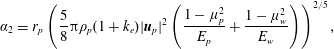
 $$\begin{eqnarray}\unicode[STIX]{x1D6FC}_{1}=r_{p,1}r_{p,2}\left({\displaystyle \frac{5}{8}}\unicode[STIX]{x03C0}\unicode[STIX]{x1D70C}_{p}(1+k_{e})|\boldsymbol{u}_{p,12}|^{2}{\displaystyle \frac{\sqrt{r_{p,1}+r_{p,2}}}{r_{p,1}^{3}+r_{p,2}^{3}}}{\displaystyle \frac{1-\unicode[STIX]{x1D707}_{p}^{2}}{E_{p}}}\right)^{2/5}.\end{eqnarray}$$
In the last expression,
 $\boldsymbol{u}_{p,12}$
is the difference between the velocities of the two colliding particles,
$\boldsymbol{u}_{p,12}$
is the difference between the velocities of the two colliding particles,
 $\boldsymbol{u}_{p,12}=\boldsymbol{u}_{p,2}-\boldsymbol{u}_{p,1}$
and
$\boldsymbol{u}_{p,12}=\boldsymbol{u}_{p,2}-\boldsymbol{u}_{p,1}$
and
 $\unicode[STIX]{x1D707}_{p}$
and
$\unicode[STIX]{x1D707}_{p}$
and
 $E_{p}$
are the Poisson ratio and the Young modulus, respectively of the material that the particulate phase is made of. Finally, the contact time
$E_{p}$
are the Poisson ratio and the Young modulus, respectively of the material that the particulate phase is made of. Finally, the contact time
 $\unicode[STIX]{x0394}t_{12}$
is also calculated by the theory of Hertz as follows,
$\unicode[STIX]{x0394}t_{12}$
is also calculated by the theory of Hertz as follows,
 $$\begin{eqnarray}\unicode[STIX]{x0394}t_{12}={\displaystyle \frac{2.94}{|\boldsymbol{u}_{p,12}|}}\unicode[STIX]{x1D6FC}_{1}.\end{eqnarray}$$
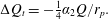
The calculation of the charge exchange during particle–wall collisions is based on the model of John, Reischl & Devor (Reference John, Reischl and Devor1980). This is derived from the model for particle–particle charge exchange of Soo (Reference Soo1971) by letting the radius of one particle go to infinity. The total charge exchange
 $\unicode[STIX]{x0394}Q$
is the sum of two contributions, namely,
$\unicode[STIX]{x0394}Q$
is the sum of two contributions, namely,
 $$\begin{eqnarray}\unicode[STIX]{x0394}Q=\unicode[STIX]{x0394}Q_{c}+\unicode[STIX]{x0394}Q_{t},\end{eqnarray}$$
where
 $\unicode[STIX]{x0394}Q_{c}$
is the dynamic charge transfer that is caused by the contact potential and
$\unicode[STIX]{x0394}Q_{c}$
is the dynamic charge transfer that is caused by the contact potential and
 $\unicode[STIX]{x0394}Q_{t}$
is the transfer of the particle pre-charge.
$\unicode[STIX]{x0394}Q_{t}$
is the transfer of the particle pre-charge.
The contact area between particle and channel wall is assumed to be much smaller than the radius of the colliding particle. Therefore, the dynamic charge transfer is modelled in a manner analogous to a charging parallel-plate capacitor. Accordingly, the particle–wall charge exchange,
 $\unicode[STIX]{x0394}Q_{c}$
, is given by
$\unicode[STIX]{x0394}Q_{c}$
, is given by
 $$\begin{eqnarray}\unicode[STIX]{x0394}Q_{c}=-CU_{c}(1-\text{e}^{-\unicode[STIX]{x0394}t_{w}/T_{w}}).\end{eqnarray}$$
In the above equation
 $C$
is the electric capacity,
$C$
is the electric capacity,
 $U_{c}$
is the particle–wall contact potential,
$U_{c}$
is the particle–wall contact potential,
 $\unicode[STIX]{x0394}t_{w}$
is the duration of the particle–wall collision and
$\unicode[STIX]{x0394}t_{w}$
is the duration of the particle–wall collision and
 $T_{w}$
is the charge relaxation time. The electric capacity of a parallel-plate capacitor is given by
$T_{w}$
is the charge relaxation time. The electric capacity of a parallel-plate capacitor is given by
 $$\begin{eqnarray}C={\displaystyle \frac{\unicode[STIX]{x1D700}_{0}A_{pw}}{h}},\end{eqnarray}$$
where
 $h$
is the distance between the plates and
$h$
is the distance between the plates and
 $A_{pw}$
is the area of the plates of the capacitor. In this sense,
$A_{pw}$
is the area of the plates of the capacitor. In this sense,
 $h$
is equal to the effective particle–wall separation during impact and
$h$
is equal to the effective particle–wall separation during impact and
 $A_{pw}$
is equal to the area of the contact surface between the particle and the wall. It is estimated according to the elastic theory of Hertz, cf. John et al. (Reference John, Reischl and Devor1980),
$A_{pw}$
is equal to the area of the contact surface between the particle and the wall. It is estimated according to the elastic theory of Hertz, cf. John et al. (Reference John, Reischl and Devor1980),
 $$\begin{eqnarray}A_{pw}=\unicode[STIX]{x03C0}r_{p}\unicode[STIX]{x1D6FC}_{2},\end{eqnarray}$$
with
 $$\begin{eqnarray}\unicode[STIX]{x1D6FC}_{2}=r_{p}\left({\displaystyle \frac{5}{8}}\unicode[STIX]{x03C0}\unicode[STIX]{x1D70C}_{p}(1+k_{e})|\boldsymbol{u}_{p}|^{2}\left({\displaystyle \frac{1-\unicode[STIX]{x1D707}_{p}^{2}}{E_{p}}}+{\displaystyle \frac{1-\unicode[STIX]{x1D707}_{w}^{2}}{E_{w}}}\right)\right)^{2/5},\end{eqnarray}$$
where
 $\unicode[STIX]{x1D707}_{w}$
and
$\unicode[STIX]{x1D707}_{w}$
and
 $E_{w}$
are the Poisson ratio and Young’s modulus, respectively, of the material of the wall. Following the arguments put forward by John et al. (Reference John, Reischl and Devor1980), the plate separation distance
$E_{w}$
are the Poisson ratio and Young’s modulus, respectively, of the material of the wall. Following the arguments put forward by John et al. (Reference John, Reischl and Devor1980), the plate separation distance
 $h$
in (2.22) is assumed to be of the order of the range of repulsive molecular forces due to surface irregularities. Herein, the theory of Hertz is also employed for the estimation of the contact time
$h$
in (2.22) is assumed to be of the order of the range of repulsive molecular forces due to surface irregularities. Herein, the theory of Hertz is also employed for the estimation of the contact time
 $\unicode[STIX]{x0394}t_{w}$
that appears in (2.21). According to this theory,
$\unicode[STIX]{x0394}t_{w}$
that appears in (2.21). According to this theory,
 $\unicode[STIX]{x0394}t_{w}$
is given by
$\unicode[STIX]{x0394}t_{w}$
is given by
 $$\begin{eqnarray}\unicode[STIX]{x0394}t_{w}={\displaystyle \frac{2.94}{|\boldsymbol{u}_{p}|}}\unicode[STIX]{x1D6FC}_{2}.\end{eqnarray}$$
Further, the charge relaxation time
 $T_{w}$
that also enters (2.21) is determined by
$T_{w}$
that also enters (2.21) is determined by
 $$\begin{eqnarray}T_{w}=\unicode[STIX]{x1D700}\unicode[STIX]{x1D700}_{0}\unicode[STIX]{x1D711}_{p},\end{eqnarray}$$
where
 $\unicode[STIX]{x1D700}$
is the relative permittivity of the system and
$\unicode[STIX]{x1D700}$
is the relative permittivity of the system and
 $\unicode[STIX]{x1D711}_{p}$
is the resistivity of the particle.
$\unicode[STIX]{x1D711}_{p}$
is the resistivity of the particle.
The pre-charge of the particle,
 $Q$
, is the charge before the collision of the particle with the wall. Herein, it is assumed to be uniformly located on its surface. Thus, the pre-charge transfer across the contact surface,
$Q$
, is the charge before the collision of the particle with the wall. Herein, it is assumed to be uniformly located on its surface. Thus, the pre-charge transfer across the contact surface,
 $\unicode[STIX]{x0394}Q_{t}$
, is given by
$\unicode[STIX]{x0394}Q_{t}$
, is given by
 $$\begin{eqnarray}\unicode[STIX]{x0394}Q_{t}=-{\textstyle \frac{1}{4}}\unicode[STIX]{x1D6FC}_{2}Q/r_{p}.\end{eqnarray}$$
It should be noted that the assumption of a uniformly distributed pre-charge is generally not valid if the particle surface is non-conducting. The effect of non-uniform charge distributions has been addressed by Grosshans & Papalexandris (Reference Grosshans and Papalexandris2016c
). However, for the cases considered herein, the charge that each particle accumulates is much smaller than its equilibrium value. Consequently, the contribution of
 $\unicode[STIX]{x0394}Q_{t}$
to the total charge transfer is small compared to
$\unicode[STIX]{x0394}Q_{t}$
to the total charge transfer is small compared to
 $\unicode[STIX]{x0394}Q_{c}$
. Therefore, the use of (2.27) is deemed appropriate for the purposes of our study.
$\unicode[STIX]{x0394}Q_{c}$
. Therefore, the use of (2.27) is deemed appropriate for the purposes of our study.
3 Numerical set-up
We consider a turbulent particle-laden flow in a channel confined by two parallel planar walls where the flow is sustained by a constant external pressure gradient. Let
 $\unicode[STIX]{x1D6FF}$
denote half the distance between the two walls and
$\unicode[STIX]{x1D6FF}$
denote half the distance between the two walls and
 $u_{c}$
the mean centreline velocity. The Reynolds number based on these quantities is
$u_{c}$
the mean centreline velocity. The Reynolds number based on these quantities is
 $Re=u_{c}\unicode[STIX]{x1D6FF}/\unicode[STIX]{x1D708}=3300$
. According to our coordinate convention, the
$Re=u_{c}\unicode[STIX]{x1D6FF}/\unicode[STIX]{x1D708}=3300$
. According to our coordinate convention, the
 $x$
-axis points to the streamwise direction, the
$x$
-axis points to the streamwise direction, the
 $y$
-axis points to the wall-normal direction and the
$y$
-axis points to the wall-normal direction and the
 $z$
-axis points to the spanwise direction.
$z$
-axis points to the spanwise direction.
As regards the fluid phase, periodic boundary conditions are applied at the streamwise and spanwise directions and the no-slip condition is applied at the two parallel walls. The initial condition consists of a fully developed turbulent flow at the aforementioned Reynolds number and randomly distributed particles whose velocities are equal to the fluid velocity at the particle locations. Following standard notation, quantities that are non-dimensionalized by the wall variables are indicated with the superscript ‘
 $+$
’. Then, the non-dimensional streamwise velocity is defined as
$+$
’. Then, the non-dimensional streamwise velocity is defined as
 $u^{+}=u/u_{\unicode[STIX]{x1D70F}}$
, where
$u^{+}=u/u_{\unicode[STIX]{x1D70F}}$
, where
 $u_{\unicode[STIX]{x1D70F}}$
is the wall friction velocity and is given in terms of the wall shear stress
$u_{\unicode[STIX]{x1D70F}}$
is the wall friction velocity and is given in terms of the wall shear stress
 $\unicode[STIX]{x1D70F}_{w}$
as
$\unicode[STIX]{x1D70F}_{w}$
as
 $u_{\unicode[STIX]{x1D70F}}=\sqrt{\unicode[STIX]{x1D70F}_{w}/\unicode[STIX]{x1D70C}}$
. Also, the distance from the wall is given by
$u_{\unicode[STIX]{x1D70F}}=\sqrt{\unicode[STIX]{x1D70F}_{w}/\unicode[STIX]{x1D70C}}$
. Also, the distance from the wall is given by
 $y^{+}=y/\unicode[STIX]{x1D6FF}_{v}$
with
$y^{+}=y/\unicode[STIX]{x1D6FF}_{v}$
with
 $\unicode[STIX]{x1D6FF}_{v}$
being the viscous length scale, i.e.
$\unicode[STIX]{x1D6FF}_{v}$
being the viscous length scale, i.e.
 $\unicode[STIX]{x1D6FF}_{v}=\unicode[STIX]{x1D708}/\sqrt{\unicode[STIX]{x1D70F}_{w}/\unicode[STIX]{x1D70C}}$
. Further, the physical time
$\unicode[STIX]{x1D6FF}_{v}=\unicode[STIX]{x1D708}/\sqrt{\unicode[STIX]{x1D70F}_{w}/\unicode[STIX]{x1D70C}}$
. Further, the physical time
 $t$
is non-dimensionalized as
$t$
is non-dimensionalized as
 $\unicode[STIX]{x1D70F}=tu_{\unicode[STIX]{x1D70F}}/\unicode[STIX]{x1D6FF}$
. Finally, the Reynolds number based on the wall friction velocity is defined as
$\unicode[STIX]{x1D70F}=tu_{\unicode[STIX]{x1D70F}}/\unicode[STIX]{x1D6FF}$
. Finally, the Reynolds number based on the wall friction velocity is defined as
 $Re_{\unicode[STIX]{x1D70F}}=u_{\unicode[STIX]{x1D70F}}\unicode[STIX]{x1D6FF}/\unicode[STIX]{x1D708}$
. On the basis of the value of
$Re_{\unicode[STIX]{x1D70F}}=u_{\unicode[STIX]{x1D70F}}\unicode[STIX]{x1D6FF}/\unicode[STIX]{x1D708}$
. On the basis of the value of
 $Re$
mentioned above, the friction Reynolds number in our simulations is
$Re$
mentioned above, the friction Reynolds number in our simulations is
 $Re_{\unicode[STIX]{x1D70F}}=180$
.
$Re_{\unicode[STIX]{x1D70F}}=180$
.
The dimensions of the computational domain in the (periodic) streamwise and spanwise directions are
 $4\unicode[STIX]{x03C0}\unicode[STIX]{x1D6FF}$
and
$4\unicode[STIX]{x03C0}\unicode[STIX]{x1D6FF}$
and
 $4/3\unicode[STIX]{x03C0}\unicode[STIX]{x1D6FF}$
, respectively; these dimensions are the same as in the studies of Wang (Reference Wang2010), Milici et al. (Reference Milici, De Marchis, Sardina and Napoli2014). In the classical paper of Kim, Moin & Moser (Reference Kim, Moin and Moser1987) the authors demonstrated that, for DNS with the given Reynolds number and a slightly larger domain in the spanwise direction, the two-point correlations of the velocity components drop to zero for sufficiently large separations in both directions. More specifically, the turbulence fluctuations were found to be uncorrelated at a separation distance of one half-period in the homogeneous directions. This is an indication that the aforementioned size of the computational domain is large enough to allow for fully developed turbulent flow with the appropriate statistical properties.
$4/3\unicode[STIX]{x03C0}\unicode[STIX]{x1D6FF}$
, respectively; these dimensions are the same as in the studies of Wang (Reference Wang2010), Milici et al. (Reference Milici, De Marchis, Sardina and Napoli2014). In the classical paper of Kim, Moin & Moser (Reference Kim, Moin and Moser1987) the authors demonstrated that, for DNS with the given Reynolds number and a slightly larger domain in the spanwise direction, the two-point correlations of the velocity components drop to zero for sufficiently large separations in both directions. More specifically, the turbulence fluctuations were found to be uncorrelated at a separation distance of one half-period in the homogeneous directions. This is an indication that the aforementioned size of the computational domain is large enough to allow for fully developed turbulent flow with the appropriate statistical properties.

Figure 1. Distribution of grid points over the half-channel width used in the present simulation compared to the set-up of Kim et al. (Reference Kim, Moin and Moser1987).
Moreover, Kim et al. (Reference Kim, Moin and Moser1987) showed that their grid resolution was sufficient for the resolution of all turbulent scales of the flow. Similarly, in our simulations we employed a non-uniform mesh in the wall-normal direction so as to adequately resolve all relevant flow structures. The minimum grid spacing is at the cells adjacent to the walls and its value is
 $\unicode[STIX]{x0394}y^{+}=0.25$
. Also, the maximum spacing is at the cells adjacent to the centreplane of the channel and its value is
$\unicode[STIX]{x0394}y^{+}=0.25$
. Also, the maximum spacing is at the cells adjacent to the centreplane of the channel and its value is
 $\unicode[STIX]{x0394}y^{+}=1.0$
. Our grid resolution in the wall-normal direction is plotted in figure 1 together with the one of Kim et al. (Reference Kim, Moin and Moser1987). From this figure, we can infer that our grid spacing is considerably finer near the centreplane, albeit a little coarser in the first 4 rows of cells. Overall, our computational grid consists of approximately eight million grid points. To reduce computing times, the code was parallelized using message passing interface and the simulations were performed in a parallel cluster.
$\unicode[STIX]{x0394}y^{+}=1.0$
. Our grid resolution in the wall-normal direction is plotted in figure 1 together with the one of Kim et al. (Reference Kim, Moin and Moser1987). From this figure, we can infer that our grid spacing is considerably finer near the centreplane, albeit a little coarser in the first 4 rows of cells. Overall, our computational grid consists of approximately eight million grid points. To reduce computing times, the code was parallelized using message passing interface and the simulations were performed in a parallel cluster.
Point-particle approaches require that the particle volume is very small compared to the volume of the smallest computational cell. In our study we have considered monodisperse particles of radius
 $r_{p}^{+}=0.1$
so that this requirement is satisfied. More specifically, one particle occupies less than 0.2 % of the volume of the smallest cell. The relevant properties of the particles and the solid walls are included in table 1. These values correspond to typical settings encountered in pneumatic powder transport in the process industries, cf. Grosshans & Papalexandris (Reference Grosshans and Papalexandris2016a
,Reference Grosshans and Papalexandris
b
).
$r_{p}^{+}=0.1$
so that this requirement is satisfied. More specifically, one particle occupies less than 0.2 % of the volume of the smallest cell. The relevant properties of the particles and the solid walls are included in table 1. These values correspond to typical settings encountered in pneumatic powder transport in the process industries, cf. Grosshans & Papalexandris (Reference Grosshans and Papalexandris2016a
,Reference Grosshans and Papalexandris
b
).
Table 1. Material properties of the particles (index
 $p$
) and channel walls (index
$p$
) and channel walls (index
 $w$
).
$w$
).

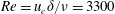
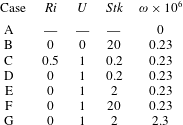
Evidently, the number of physical parameters involved in the flows under consideration is quite large. In our study we focused on the influence of three important non-dimensional parameters, namely, the particle Stokes number
 $Stk$
, the Richardson number
$Stk$
, the Richardson number
 $Ri$
and the volume fraction of the particulate phase
$Ri$
and the volume fraction of the particulate phase
 $\unicode[STIX]{x1D714}$
. Their values for all cases considered in our study are listed in table 2. It should be mentioned that case A corresponds to a single-phase flow (in the absence of particles), whereas case B corresponds to a particle-laden flow without electrostatic charging. Both of these cases have been introduced for comparison purposes.
$\unicode[STIX]{x1D714}$
. Their values for all cases considered in our study are listed in table 2. It should be mentioned that case A corresponds to a single-phase flow (in the absence of particles), whereas case B corresponds to a particle-laden flow without electrostatic charging. Both of these cases have been introduced for comparison purposes.
Table 2. Summary of the non-dimensional parameters for the cases considered in our study.
In our simulations with gravity we consider that the gravity vector points in the opposite direction to the
 $y$
-axis, i.e.
$y$
-axis, i.e.
 $\boldsymbol{g}=(0,-g,0)$
. The Richardson number is defined as
$\boldsymbol{g}=(0,-g,0)$
. The Richardson number is defined as
 $Ri=g\unicode[STIX]{x1D6FF}/u_{c}^{2}$
. By performing DNS of particle-laden turbulent flow in a vertical channel at
$Ri=g\unicode[STIX]{x1D6FF}/u_{c}^{2}$
. By performing DNS of particle-laden turbulent flow in a vertical channel at
 $Re_{\unicode[STIX]{x1D70F}}=150$
, Marchioli, Picciotto & Soldati (Reference Marchioli, Picciotto and Soldati2007) analysed the effects of gravity on particle dispersion and deposition. They reported that for particles smaller than
$Re_{\unicode[STIX]{x1D70F}}=150$
, Marchioli, Picciotto & Soldati (Reference Marchioli, Picciotto and Soldati2007) analysed the effects of gravity on particle dispersion and deposition. They reported that for particles smaller than
 $r_{p}^{+}=0.3$
, the particle statistics with and without gravity were nearly identical. On the basis of these results, and in order to focus on particle–fluid interactions, the cases considered in our study assume
$r_{p}^{+}=0.3$
, the particle statistics with and without gravity were nearly identical. On the basis of these results, and in order to focus on particle–fluid interactions, the cases considered in our study assume
 $Ri=0$
, with the exception of case C for which the Richardson number was set to
$Ri=0$
, with the exception of case C for which the Richardson number was set to
 $Ri=0.5$
. Case C was introduced in order to explore the effect of the gravitational acceleration
$Ri=0.5$
. Case C was introduced in order to explore the effect of the gravitational acceleration
 $\boldsymbol{f}_{g}$
on triboelectric charging in a horizontal channel.
$\boldsymbol{f}_{g}$
on triboelectric charging in a horizontal channel.
Also, as regards the contact potential
 $U_{c}$
, it is non-dimensionalized by a reference potential
$U_{c}$
, it is non-dimensionalized by a reference potential
 $U_{0}$
that is set equal to 1 V. In all cases with particle electrification considered herein, the value of the non-dimensional contact potential
$U_{0}$
that is set equal to 1 V. In all cases with particle electrification considered herein, the value of the non-dimensional contact potential
 $U$
is set equal to unity, i.e.
$U$
is set equal to unity, i.e.
 $U=U_{c}/U_{0}=1$
.
$U=U_{c}/U_{0}=1$
.
The particle Stokes number
 $Stk$
is defined as the ratio between the particle response time
$Stk$
is defined as the ratio between the particle response time
 $T_{r}$
and the characteristic time scale of the fluid flow,
$T_{r}$
and the characteristic time scale of the fluid flow,
 $T_{f}$
, i.e.
$T_{f}$
, i.e.
 $Stk=T_{r}/T_{f}$
. In the literature, several different approaches for the estimation of
$Stk=T_{r}/T_{f}$
. In the literature, several different approaches for the estimation of
 $T_{r}$
and
$T_{r}$
and
 $T_{f}$
are available; see for example, Israel & Rosner (Reference Israel and Rosner1982). Herein,
$T_{f}$
are available; see for example, Israel & Rosner (Reference Israel and Rosner1982). Herein,
 $T_{f}$
is defined in terms of the channel half-width
$T_{f}$
is defined in terms of the channel half-width
 $\unicode[STIX]{x1D6FF}$
and the centreline velocity,
$\unicode[STIX]{x1D6FF}$
and the centreline velocity,
 $T_{f}=\unicode[STIX]{x1D6FF}/u_{c}$
. As regards
$T_{f}=\unicode[STIX]{x1D6FF}/u_{c}$
. As regards
 $T_{r}$
, we employ the common assumption of low particle Reynolds number (Stiesch Reference Stiesch2003; Crowe et al.
Reference Crowe, Schwarzkopf, Sommerfeld and Tsuji2012). Consequently, the Stokes’ law of drag is valid and the particle response time can be estimated by
$T_{r}$
, we employ the common assumption of low particle Reynolds number (Stiesch Reference Stiesch2003; Crowe et al.
Reference Crowe, Schwarzkopf, Sommerfeld and Tsuji2012). Consequently, the Stokes’ law of drag is valid and the particle response time can be estimated by
 $$\begin{eqnarray}T_{r}=\frac{2}{9}\frac{\unicode[STIX]{x1D70C}_{p}}{\unicode[STIX]{x1D70C}}\frac{r_{p}^{2}}{\unicode[STIX]{x1D708}}.\end{eqnarray}$$
When the Stokes number is much larger than unity, the particle trajectories are hardly disturbed by the fluid flow. On the contrary, if it is much smaller than unity, then the particle trajectories follow closely the flow streamlines. In order to investigate the influence of the particle dynamics on the charge build-up, we considered cases with three different Stokes numbers, namely
 $Stk=0.2$
, 2 and 20.
$Stk=0.2$
, 2 and 20.
Finally, with respect to the flow domain, the volume fraction of the particulate phase
 $\unicode[STIX]{x1D714}$
is given by
$\unicode[STIX]{x1D714}$
is given by
 $$\begin{eqnarray}\unicode[STIX]{x1D714}=\frac{V_{p}}{V}=\frac{N}{8\unicode[STIX]{x03C0}}\frac{r_{p}^{3}}{\unicode[STIX]{x1D6FF}^{3}},\end{eqnarray}$$
where
 $V_{p}$
is the total volume occupied by the particles,
$V_{p}$
is the total volume occupied by the particles,
 $V$
is the volume of the flow domain and
$V$
is the volume of the flow domain and
 $N$
stands for the total number of particles in the domain. In all cases, except for case G, we considered
$N$
stands for the total number of particles in the domain. In all cases, except for case G, we considered
 $\unicode[STIX]{x1D714}=0.23\times 10^{-6}$
which corresponds to
$\unicode[STIX]{x1D714}=0.23\times 10^{-6}$
which corresponds to
 $N=40\,000$
. In case G the total number of particles was increased by a factor of 10, i.e.
$N=40\,000$
. In case G the total number of particles was increased by a factor of 10, i.e.
 $N=400\,000$
. Finally, as mentioned above, in case A there were no particles at all.
$N=400\,000$
. Finally, as mentioned above, in case A there were no particles at all.
4 Presentation and discussion of the numerical results
In this section we first provide the results of the simulations and tests that we performed in order to validate our solver. Subsequently, we present and discuss in detail the results of our simulations of triboelectric charging.
4.1 Validation of the solver
The implementation of the Eulerian solver for the fluid phase has been validated by comparing our results for case A (cf. table 2) with the DNS data of the classical paper of Kim et al. (Reference Kim, Moin and Moser1987) and with the experimental studies of Eckelmann (Reference Eckelmann1974) and Kreplin & Eckelmann (Reference Kreplin and Eckelmann1979). The profiles of the mean streamwise velocity component
 $\langle u^{+}\rangle$
, i.e. averaged in time and in the homogeneous directions, are depicted in figure 2. According to this figure, our numerical results compare very well with the earlier DNS and experimental data. Actually, the experiments of Eckelmann (Reference Eckelmann1974) were conducted at a slightly different Reynolds number,
$\langle u^{+}\rangle$
, i.e. averaged in time and in the homogeneous directions, are depicted in figure 2. According to this figure, our numerical results compare very well with the earlier DNS and experimental data. Actually, the experiments of Eckelmann (Reference Eckelmann1974) were conducted at a slightly different Reynolds number,
 $Re=2800$
which corresponds to
$Re=2800$
which corresponds to
 $Re_{\unicode[STIX]{x1D70F}}=142$
. For this reason, in their paper, Kim et al. (Reference Kim, Moin and Moser1987) rescaled the mean streamwise velocity profile of Eckelmann (Reference Eckelmann1974) in such a way that they agree with the results of Wallace, Eckelmann & Brodkey (Reference Wallace, Eckelmann and Brodkey1972) at
$Re_{\unicode[STIX]{x1D70F}}=142$
. For this reason, in their paper, Kim et al. (Reference Kim, Moin and Moser1987) rescaled the mean streamwise velocity profile of Eckelmann (Reference Eckelmann1974) in such a way that they agree with the results of Wallace, Eckelmann & Brodkey (Reference Wallace, Eckelmann and Brodkey1972) at
 $y^{+}=100$
. The curves given in figure 2 correspond to the rescaled data. The profiles of the root-mean-square (r.m.s.) fluctuations of the three velocity components are plotted in figure 3. Again, we can verify that our numerical results agree very well with the earlier DNS and experimental data that were cited above.
$y^{+}=100$
. The curves given in figure 2 correspond to the rescaled data. The profiles of the root-mean-square (r.m.s.) fluctuations of the three velocity components are plotted in figure 3. Again, we can verify that our numerical results agree very well with the earlier DNS and experimental data that were cited above.

Figure 2. Profiles of the mean streamwise velocity
 $\langle u^{+}\rangle$
for case A (single-phase flow), expressed in wall units. Comparison of our numerical results with the numerical results of Kim et al. (Reference Kim, Moin and Moser1987) and the experimental data of Eckelmann (Reference Eckelmann1974). The experimental data have been rescaled according to Kim et al. (Reference Kim, Moin and Moser1987).
$\langle u^{+}\rangle$
for case A (single-phase flow), expressed in wall units. Comparison of our numerical results with the numerical results of Kim et al. (Reference Kim, Moin and Moser1987) and the experimental data of Eckelmann (Reference Eckelmann1974). The experimental data have been rescaled according to Kim et al. (Reference Kim, Moin and Moser1987).
The one-dimensional energy spectra of each velocity component obtained by our simulations are compared with those from the DNS results of Kim et al. (Reference Kim, Moin and Moser1987) in figure 4. We can clearly see that, once again, a very good agreement is observed for the spectra of all velocity components.
The electrostatics model has been validated via comparisons with the experimental data of Matsuyama & Yamamoto (Reference Matsuyama and Yamamoto1995) who measured the charge exchange during collisions of particles with a solid target. According to our comparisons, which are described in Grosshans & Papalexandris (Reference Grosshans and Papalexandris2016c ), the model can accurately predict both the amount of the exchanged charge and its dependency to the particle charge prior to impact.

Figure 3. Profiles of r.m.s. velocity fluctuations for case A (single-phase flow). Comparison of our numerical results with the numerical results of Kim et al. (Reference Kim, Moin and Moser1987) and the experimental data of Eckelmann (Reference Eckelmann1974). The empty symbols are used for the r.m.s. fluctuations of the streamwise velocity component
 $u_{rms}^{+}$
, the black symbols for the r.m.s. fluctuations of the wall-normal component
$u_{rms}^{+}$
, the black symbols for the r.m.s. fluctuations of the wall-normal component
 $v_{rms}^{+}$
, and the grey symbols for the r.m.s. fluctuations of the spanwise velocity component
$v_{rms}^{+}$
, and the grey symbols for the r.m.s. fluctuations of the spanwise velocity component
 $w_{rms}^{+}$
.
$w_{rms}^{+}$
.

Figure 4. One-dimensional energy spectra for case A (single-phase flow). Comparison of our numerical results with those of Kim et al. (Reference Kim, Moin and Moser1987). (a)
 $E_{uu}$
, (b)
$E_{uu}$
, (b)
 $E_{vv}$
and (c)
$E_{vv}$
and (c)
 $E_{ww}$
. The spectra are evaluated at
$E_{ww}$
. The spectra are evaluated at
 $y/\unicode[STIX]{x1D6FF}=0.829$
, which corresponds to
$y/\unicode[STIX]{x1D6FF}=0.829$
, which corresponds to
 $y^{+}=149.23$
.
$y^{+}=149.23$
.
4.2 Simulations of triboelectric charging
Once the hydrodynamics and electrostatics solver was validated, we performed direct numerical simulations of triboelectric charging in a turbulent channel flow. Our initial condition consists of a fully developed turbulent field (taken from the simulation of case A) and a random distribution of particles. The duration of each simulation was 12 non-dimensional time units.

Figure 5. Instantaneous visualizations of the flow patterns of case F (
 $Ri=0$
,
$Ri=0$
,
 $U=1$
,
$U=1$
,
 $Stk=20$
,
$Stk=20$
,
 $\unicode[STIX]{x1D714}=0.23\times 10^{-6}$
). The black contours represent the isolines of the magnitude of the fluid velocity. For visualization purposes, the particles are enlarged and only every other particle is shown. The
$\unicode[STIX]{x1D714}=0.23\times 10^{-6}$
). The black contours represent the isolines of the magnitude of the fluid velocity. For visualization purposes, the particles are enlarged and only every other particle is shown. The
 $x$
-axis points in the streamwise direction and the
$x$
-axis points in the streamwise direction and the
 $y$
-axis in the wall-normal direction.
$y$
-axis in the wall-normal direction.
An instantaneous fluid flow field for case F (which corresponds to a high Stokes number) is depicted in figure 5. The charge and location of the particles are also provided in this figure. For visualization purposes, the particles are enlarged and only every other particle is shown. Further, in figure 5 and throughout this paper, the particle charge is expressed in terms of the absolute non-dimensional specific charge
 $\unicode[STIX]{x1D70E}$
which is defined as
$\unicode[STIX]{x1D70E}$
which is defined as
 $$\begin{eqnarray}\unicode[STIX]{x1D70E}={\displaystyle \frac{|Q|U_{0}}{m_{p}u_{c}^{2}}}.\end{eqnarray}$$
In the above definition, we have used the absolute value of the particle charge
 $|Q|$
due to the uncertainty on the polarity of the surface potential. It can be inferred that, for both time instances shown in figure 5, the particles near the walls carry, on average, a higher charge than the particles located in the bulk of the channel. However, the number of highly charged particles located far from the walls increases between
$|Q|$
due to the uncertainty on the polarity of the surface potential. It can be inferred that, for both time instances shown in figure 5, the particles near the walls carry, on average, a higher charge than the particles located in the bulk of the channel. However, the number of highly charged particles located far from the walls increases between
 $\unicode[STIX]{x1D70F}=5$
and
$\unicode[STIX]{x1D70F}=5$
and
 $\unicode[STIX]{x1D70F}=10$
. This implies that, upon collision with the walls, the particles accumulate charge and subsequently migrate towards the bulk of the channel while carrying with them the accumulated electric charge. Herein we refer to this phenomenon as particle-bound charge transport.
$\unicode[STIX]{x1D70F}=10$
. This implies that, upon collision with the walls, the particles accumulate charge and subsequently migrate towards the bulk of the channel while carrying with them the accumulated electric charge. Herein we refer to this phenomenon as particle-bound charge transport.
Also, from figure 5 it can be inferred that the overall number of particles in the vicinity of the centreplane decreases with time. Further, the particles adopt a preferential location close to the walls. This is the phenomenon of turbophoretic drift that has been discussed in the introduction of this paper. It becomes clear that particle-bound charge transport and turbophoretic drift are counter-acting mechanisms, as regards the charging patterns and distribution of electric charge across the channel. The interplay between these two mechanisms and its role to the electrification of the particulate phase are elaborated below.
4.3 Influence of the Stokes number
In figure 6 we provide plots of the average particle charge, defined as
 $$\begin{eqnarray}\bar{\unicode[STIX]{x1D70E}}=\frac{1}{N}\mathop{\sum }_{i=1}^{N}\unicode[STIX]{x1D70E}_{i},\end{eqnarray}$$
for cases with different Stokes numbers. An increase of the Stokes number implies that the particles are affected less by the flow structures, resulting in a higher frequency of particle–wall collisions. This, in turn, leads to a significant increase of the charging rate of the particulate phase.

Figure 6. Average particle charge
 $\bar{\unicode[STIX]{x1D70E}}$
for cases D, E and F (
$\bar{\unicode[STIX]{x1D70E}}$
for cases D, E and F (
 $Ri=0$
,
$Ri=0$
,
 $U=1$
and
$U=1$
and
 $\unicode[STIX]{x1D714}=0.23\times 10^{-6}$
). An increase of the Stokes number results in an increase of the charging rate of the particulate phase.
$\unicode[STIX]{x1D714}=0.23\times 10^{-6}$
). An increase of the Stokes number results in an increase of the charging rate of the particulate phase.

Figure 7. Evolution of the profiles of the linear particle number density
 $\unicode[STIX]{x1D6FD}$
for case D (
$\unicode[STIX]{x1D6FD}$
for case D (
 $Ri=0$
,
$Ri=0$
,
 $U=1$
,
$U=1$
,
 $Stk=0.2$
and
$Stk=0.2$
and
 $\unicode[STIX]{x1D714}=0.23\times 10^{-6}$
). The preferential particle concentrations between
$\unicode[STIX]{x1D714}=0.23\times 10^{-6}$
). The preferential particle concentrations between
 $y^{+}=1$
and
$y^{+}=1$
and
 $y^{+}=5$
provide evidence of the phenomenon of turbophoresis.
$y^{+}=5$
provide evidence of the phenomenon of turbophoresis.
More specifically, in the case of low Stokes number, case D with
 $Stk=0.2$
, the amount of electric charge accumulated by the particles is negligible, as can be directly confirmed from figure 6. The profiles of the linear particle number density
$Stk=0.2$
, the amount of electric charge accumulated by the particles is negligible, as can be directly confirmed from figure 6. The profiles of the linear particle number density
 $\unicode[STIX]{x1D6FD}$
, defined as number of particles per viscous length scale
$\unicode[STIX]{x1D6FD}$
, defined as number of particles per viscous length scale
 $\unicode[STIX]{x1D6FF}_{v}$
in the wall-normal direction, for this case and at times
$\unicode[STIX]{x1D6FF}_{v}$
in the wall-normal direction, for this case and at times
 $\unicode[STIX]{x1D70F}=0.75$
, 6.75 and 12.0 are depicted in figure 7. Since for all cases without gravity the flow is statistically symmetric with respect to the channel centreplane, figure 7 shows only the profiles of
$\unicode[STIX]{x1D70F}=0.75$
, 6.75 and 12.0 are depicted in figure 7. Since for all cases without gravity the flow is statistically symmetric with respect to the channel centreplane, figure 7 shows only the profiles of
 $\unicode[STIX]{x1D6FD}$
across half of the channel. These plots confirm that there are very few particles in the region
$\unicode[STIX]{x1D6FD}$
across half of the channel. These plots confirm that there are very few particles in the region
 $0<y^{+}<0.1$
, which excludes the possibility of particle–wall collisions and, consequently, particle charging. This is a direct consequence of the fact that, at low Stokes numbers, the particles follow closely the flow streamlines. Furthermore, very close to the wall, the flow streamlines are almost parallel to it and so are the particle trajectories. Therefore, particle–wall collisions become exceedingly improbable below a certain Stokes number. Similar predictions were made earlier by Cleaver & Yates (Reference Cleaver and Yates1975).
$0<y^{+}<0.1$
, which excludes the possibility of particle–wall collisions and, consequently, particle charging. This is a direct consequence of the fact that, at low Stokes numbers, the particles follow closely the flow streamlines. Furthermore, very close to the wall, the flow streamlines are almost parallel to it and so are the particle trajectories. Therefore, particle–wall collisions become exceedingly improbable below a certain Stokes number. Similar predictions were made earlier by Cleaver & Yates (Reference Cleaver and Yates1975).
Moreover, according to figure 7, the profiles of the linear particle number density have peaks located between
 $y^{+}=1$
and
$y^{+}=1$
and
 $y^{+}=5$
. We also note that as time goes by, the peak value grows and the peak location is shifted slowly closer to the wall. On the other hand, far from the wall,
$y^{+}=5$
. We also note that as time goes by, the peak value grows and the peak location is shifted slowly closer to the wall. On the other hand, far from the wall,
 $y^{+}>10$
, the profile of
$y^{+}>10$
, the profile of
 $\unicode[STIX]{x1D6FD}$
remains almost constant and its value is less than half of the maximum. This is a manifestation of the aforementioned phenomenon of turbophoresis.
$\unicode[STIX]{x1D6FD}$
remains almost constant and its value is less than half of the maximum. This is a manifestation of the aforementioned phenomenon of turbophoresis.
Next, we examine the charging curve for case E, i.e. when the Stokes number was increased to 2 while keeping the other parameters constant. As can be ascertained from figure 6, the charging of particles in this case is noteworthy. In fact, as mentioned by Eaton (Reference Eaton2009), at moderate Stokes numbers the coupling between the carrier fluid and the particulate phase via momentum exchange is substantial and the particles no longer follow closely the fluid streamlines. Accordingly, the frequency of particle–wall collisions is sufficiently high to cause significant particle electrification. Evidently, the charge increases monotonically with time; nonetheless, the charging rate exhibits some small fluctuations, as can be inferred upon inspection of the plot in figure 6. These are due to variations of the particle–wall collision frequency and may be attributed to the effect of the turbulent structures of the flow to the particle trajectories.

Figure 8. Evolution of the profiles of the linear particle number density
 $\unicode[STIX]{x1D6FD}$
for case E (
$\unicode[STIX]{x1D6FD}$
for case E (
 $Ri=0$
,
$Ri=0$
,
 $U=1$
,
$U=1$
,
 $Stk=2$
and
$Stk=2$
and
 $\unicode[STIX]{x1D714}=0.23\times 10^{-6}$
). It can be inferred that, compared to case D of lower
$\unicode[STIX]{x1D714}=0.23\times 10^{-6}$
). It can be inferred that, compared to case D of lower
 $Stk$
, the location of the peak value of
$Stk$
, the location of the peak value of
 $\unicode[STIX]{x1D6FD}$
is shifted towards the wall.
$\unicode[STIX]{x1D6FD}$
is shifted towards the wall.
The profiles of the linear particle number density
 $\unicode[STIX]{x1D6FD}$
for case E are shown in figure 8. As in the previous case, the effect of turbophoresis, i.e. particle agglomeration in the viscous sublayer, can readily be observed. Further, similar to case D, the peak value of the particle number density increases with time whereas far from the walls
$\unicode[STIX]{x1D6FD}$
for case E are shown in figure 8. As in the previous case, the effect of turbophoresis, i.e. particle agglomeration in the viscous sublayer, can readily be observed. Further, similar to case D, the peak value of the particle number density increases with time whereas far from the walls
 $\unicode[STIX]{x1D6FD}$
remains approximately constant.
$\unicode[STIX]{x1D6FD}$
remains approximately constant.
Nonetheless, there are several significant differences between cases D and E. First, according to the profiles presented in figure 8, the ratio between the peak value of
 $\unicode[STIX]{x1D6FD}$
and the value close to the centreplane of the channel is much higher in case E than in case D. In fact, the ratio between the particle concentrations at the location of the peaks and at the centreplane is several orders of magnitude higher for
$\unicode[STIX]{x1D6FD}$
and the value close to the centreplane of the channel is much higher in case E than in case D. In fact, the ratio between the particle concentrations at the location of the peaks and at the centreplane is several orders of magnitude higher for
 $Stk=2$
. In other words, as we pass from low to moderate Stokes numbers, the phenomenon of turbophoresis becomes more pronounced. Conversely, as
$Stk=2$
. In other words, as we pass from low to moderate Stokes numbers, the phenomenon of turbophoresis becomes more pronounced. Conversely, as
 $Stk$
approaches zero, we anticipate a uniform particle distribution across the channel and disappearance of turbophoresis. This is explained by the fact that, at vanishing Stokes number, the solid particles behave as passive scalars that are convected by the flow; see also the discussion of Brooke et al. (Reference Brooke, Kontomaris, Hanratty and McLaughlin1992).
$Stk$
approaches zero, we anticipate a uniform particle distribution across the channel and disappearance of turbophoresis. This is explained by the fact that, at vanishing Stokes number, the solid particles behave as passive scalars that are convected by the flow; see also the discussion of Brooke et al. (Reference Brooke, Kontomaris, Hanratty and McLaughlin1992).
Another noticeable difference is that for higher
 $Stk$
(case E) the location of the peak value of
$Stk$
(case E) the location of the peak value of
 $\unicode[STIX]{x1D6FD}$
is significantly shifted towards the wall. More specifically, in case E the peak is located between
$\unicode[STIX]{x1D6FD}$
is significantly shifted towards the wall. More specifically, in case E the peak is located between
 $y^{+}=0.3$
and
$y^{+}=0.3$
and
 $y^{+}=0.4$
, whereas in case D it is located beyond
$y^{+}=0.4$
, whereas in case D it is located beyond
 $y^{+}=1$
. More important, according to figure 8, the number of particles very close to the wall is much higher in case E than in case D and increases even further with time. This results in a significant increase of the frequency of particle–wall collisions which translates directly to higher charging rates, cf. figure 6.
$y^{+}=1$
. More important, according to figure 8, the number of particles very close to the wall is much higher in case E than in case D and increases even further with time. This results in a significant increase of the frequency of particle–wall collisions which translates directly to higher charging rates, cf. figure 6.

Figure 9. Evolution of the profiles of the linear charge density
 $\unicode[STIX]{x1D6FE}$
for case E (
$\unicode[STIX]{x1D6FE}$
for case E (
 $Ri=0$
,
$Ri=0$
,
 $U=1$
,
$U=1$
,
 $Stk=2$
and
$Stk=2$
and
 $\unicode[STIX]{x1D714}=0.23\times 10^{-6}$
). The charged particles, hence the electrostatic charge, migrate away from the wall. However, this process is so slow that the electric charge remains practically confined within a thin layer very close to the wall.
$\unicode[STIX]{x1D714}=0.23\times 10^{-6}$
). The charged particles, hence the electrostatic charge, migrate away from the wall. However, this process is so slow that the electric charge remains practically confined within a thin layer very close to the wall.
Also for case E, the resulting profiles of the linear charge density
 $\unicode[STIX]{x1D6FE}$
, defined as charge per viscous length scale
$\unicode[STIX]{x1D6FE}$
, defined as charge per viscous length scale
 $\unicode[STIX]{x1D6FF}_{v}$
in the wall-normal direction, are plotted in figure 9. From these plots we can infer that the charge next to the wall increases with time. In general, upon collision with the wall, the charged particles, hence the electrostatic charge, migrate towards the bulk of the channel. Nonetheless, this process is very slow so that the electric charge remains practically confined within a thin layer very close to the wall. More specifically, throughout the duration of the simulation, the region defined by
$\unicode[STIX]{x1D6FF}_{v}$
in the wall-normal direction, are plotted in figure 9. From these plots we can infer that the charge next to the wall increases with time. In general, upon collision with the wall, the charged particles, hence the electrostatic charge, migrate towards the bulk of the channel. Nonetheless, this process is very slow so that the electric charge remains practically confined within a thin layer very close to the wall. More specifically, throughout the duration of the simulation, the region defined by
 $y^{+}>1$
remained uncharged so that one may assume that even at later times most of the electric charge is still located in the viscous sublayer. This means that the particle electrification is dominated by particle–wall collisions. On the contrary, the transport of charge towards the bulk of the channel via particle-bound charge transport or via inter-particle collisions is much weaker.
$y^{+}>1$
remained uncharged so that one may assume that even at later times most of the electric charge is still located in the viscous sublayer. This means that the particle electrification is dominated by particle–wall collisions. On the contrary, the transport of charge towards the bulk of the channel via particle-bound charge transport or via inter-particle collisions is much weaker.
Next, we discuss our numerical predictions for case F which corresponds to a high Stokes number,
 $Stk=20$
. As can be seen in figure 6, this case is characterized by a significant increase in the charging rate of particles. Moreover, whereas for
$Stk=20$
. As can be seen in figure 6, this case is characterized by a significant increase in the charging rate of particles. Moreover, whereas for
 $Stk=2$
the charging rate exhibits some fluctuations, for
$Stk=2$
the charging rate exhibits some fluctuations, for
 $Stk=20$
it is almost constant. In other words, the particle charge increases linearly with time. In fact, at high
$Stk=20$
it is almost constant. In other words, the particle charge increases linearly with time. In fact, at high
 $Stk$
, particle dynamics is dominated by the inertia of the particles and their trajectories are slightly perturbed by the flow turbulence. This implies that the frequency of particle–wall collisions remains (almost) constant, which explains the predicted constancy of the charging rate of the particulate phase.
$Stk$
, particle dynamics is dominated by the inertia of the particles and their trajectories are slightly perturbed by the flow turbulence. This implies that the frequency of particle–wall collisions remains (almost) constant, which explains the predicted constancy of the charging rate of the particulate phase.
Upon comparison of the linear particle number density profiles in figure 10 with those in figures 7 and 8, we infer that the process of particle agglomeration in a thin region close to the walls advances more slowly, in the sense that the gradients of
 $\unicode[STIX]{x1D6FD}$
are not as steep as in the previous cases. This can be explained as follows. First we remark that the characteristic turbulence time scale decreases progressively in the normal direction as we approach the wall. However, high-density particles have a longer response time scale. Consequently, the trajectories of these particles are not perturbed significantly by the smaller turbulent structures. Therefore, upon impact with the walls, the momentum of these particles in the wall-normal direction is sufficient for some of them to cross the viscous sublayer without getting trapped by the near-wall structures of the flow. This is also in accordance with the numerical predictions of Marchioli & Soldati (Reference Marchioli and Soldati2002) for uncharged gravity-driven flows who proposed an explanation for this phenomenon on the basis of the increase of the local Stokes number for particles of a higher inertia.
$\unicode[STIX]{x1D6FD}$
are not as steep as in the previous cases. This can be explained as follows. First we remark that the characteristic turbulence time scale decreases progressively in the normal direction as we approach the wall. However, high-density particles have a longer response time scale. Consequently, the trajectories of these particles are not perturbed significantly by the smaller turbulent structures. Therefore, upon impact with the walls, the momentum of these particles in the wall-normal direction is sufficient for some of them to cross the viscous sublayer without getting trapped by the near-wall structures of the flow. This is also in accordance with the numerical predictions of Marchioli & Soldati (Reference Marchioli and Soldati2002) for uncharged gravity-driven flows who proposed an explanation for this phenomenon on the basis of the increase of the local Stokes number for particles of a higher inertia.

Figure 10. Evolution of the profiles of the linear particle number density
 $\unicode[STIX]{x1D6FD}$
for case F (
$\unicode[STIX]{x1D6FD}$
for case F (
 $Ri=0$
,
$Ri=0$
,
 $U=1$
,
$U=1$
,
 $Stk=20$
and
$Stk=20$
and
 $\unicode[STIX]{x1D714}=0.23\times 10^{-6}$
). The process of particle agglomeration in a thin region close to the walls advances more slowly. Further, the number of particles that lie between the wall and the location of maximum number density is higher.
$\unicode[STIX]{x1D714}=0.23\times 10^{-6}$
). The process of particle agglomeration in a thin region close to the walls advances more slowly. Further, the number of particles that lie between the wall and the location of maximum number density is higher.
The peaks of the linear particle number density profiles shown in figure 10 are located in the region
 $0.1<y^{+}<0.3$
, i.e. closer to the wall than in the previous cases. Also, the number of particles that lie between the wall and the location of maximum number density is higher as the Stokes number increases, which is consistent with the above analysis of particle transport in the wall-normal direction. This causes a significantly different charge distribution for
$0.1<y^{+}<0.3$
, i.e. closer to the wall than in the previous cases. Also, the number of particles that lie between the wall and the location of maximum number density is higher as the Stokes number increases, which is consistent with the above analysis of particle transport in the wall-normal direction. This causes a significantly different charge distribution for
 $Stk=20$
when compared to the other cases, as can be seen in figure 11. In particular, we observe that at
$Stk=20$
when compared to the other cases, as can be seen in figure 11. In particular, we observe that at
 $\unicode[STIX]{x1D70F}=12$
the linear charge density
$\unicode[STIX]{x1D70F}=12$
the linear charge density
 $\unicode[STIX]{x1D6FE}$
has a peak at the location of the preferential particle concentration, i.e.
$\unicode[STIX]{x1D6FE}$
has a peak at the location of the preferential particle concentration, i.e.
 $0.2<y^{+}<0.3$
, whereas in the previous cases the peak of
$0.2<y^{+}<0.3$
, whereas in the previous cases the peak of
 $\unicode[STIX]{x1D6FE}$
is adjacent to the wall, cf. figure 9. Moreover, a significant amount of charge is transported towards the bulk of the channel via particle-bound transport.
$\unicode[STIX]{x1D6FE}$
is adjacent to the wall, cf. figure 9. Moreover, a significant amount of charge is transported towards the bulk of the channel via particle-bound transport.

Figure 11. Evolution of the profiles of the linear charge density
 $\unicode[STIX]{x1D6FE}$
for case F (
$\unicode[STIX]{x1D6FE}$
for case F (
 $Ri=0$
,
$Ri=0$
,
 $U=1$
,
$U=1$
,
 $Stk=20$
and
$Stk=20$
and
 $\unicode[STIX]{x1D714}=0.23\times 10^{-6}$
). At high Stokes numbers, a significant amount of electric charge migrates towards the centreplane of the channel via particle-bound charge transport.
$\unicode[STIX]{x1D714}=0.23\times 10^{-6}$
). At high Stokes numbers, a significant amount of electric charge migrates towards the centreplane of the channel via particle-bound charge transport.

Figure 12. Profiles of the r.m.s. fluctuations of the particle velocity components. (a) Streamwise component, (b) wall-normal component, (c) spanwise component. While the fluctuations of the streamwise component are very similar for all cases, the fluctuations of the wall-normal and spanwise components increase as the Stokes number is decreased.

Figure 13. Profiles of the fluctuations of the wall-normal particle velocities close to the wall.
These observations can be corroborated further upon examination of the statistics of the particle velocities. To this end, in figure 12 we present the r.m.s. fluctuations of the particle velocity components,
 $u_{p,rms}$
,
$u_{p,rms}$
,
 $v_{p,rms}$
and
$v_{p,rms}$
and
 $w_{p,rms}$
, at
$w_{p,rms}$
, at
 $\unicode[STIX]{x1D70F}=12$
for all cases without gravity that were considered in our study. The first remark is that the electric force is too weak to influence the particle dynamics, as can be evidenced by comparing the curves for case B with
$\unicode[STIX]{x1D70F}=12$
for all cases without gravity that were considered in our study. The first remark is that the electric force is too weak to influence the particle dynamics, as can be evidenced by comparing the curves for case B with
 $U=0$
and for the equivalent case F with
$U=0$
and for the equivalent case F with
 $U=1$
. This is related to the fact that our study focuses on the transient phase (build-up) of triboelectric charging and during this phase the accumulated charge is still small. Consequently, the strength of the electrical field remains low.
$U=1$
. This is related to the fact that our study focuses on the transient phase (build-up) of triboelectric charging and during this phase the accumulated charge is still small. Consequently, the strength of the electrical field remains low.
We also observe that the particle velocity fluctuations have globally the same trends as the ones of the fluid velocity, cf. figure 3. Also, due to particle inertia, the r.m.s. fluctuations of the particle velocities are generally lower than those of the fluid, except for locations adjacent to the wall since the particles are not subject to the zero slip condition.
However, we remark that, even though the fluctuations of the streamwise velocity component are very similar for all cases, the fluctuations of the wall-normal and spanwise components increase as the Stokes number decreases. This is attributed to the fact that at lower
 $Stk$
, the particles adapt faster to the fluid velocity and are, therefore, more sensitive to the turbulent structures of the flow. On the other hand, at high Stokes number the trajectories of the particles become more ballistic and, therefore, insensitive to turbulent fluctuations.
$Stk$
, the particles adapt faster to the fluid velocity and are, therefore, more sensitive to the turbulent structures of the flow. On the other hand, at high Stokes number the trajectories of the particles become more ballistic and, therefore, insensitive to turbulent fluctuations.
However, the dependence of the
 $v_{p,rms}$
fluctuations with the Stokes number close to the wall exhibits the opposite trend, in accordance with the mechanism of particle-bound charge transport that was elaborated above. To verify this, we zoomed on the profiles of
$v_{p,rms}$
fluctuations with the Stokes number close to the wall exhibits the opposite trend, in accordance with the mechanism of particle-bound charge transport that was elaborated above. To verify this, we zoomed on the profiles of
 $v_{p,rms}$
in the region
$v_{p,rms}$
in the region
 $y^{+}<2$
, as shown in figure 13. In this figure we see that as the Stokes number decreases, the
$y^{+}<2$
, as shown in figure 13. In this figure we see that as the Stokes number decreases, the
 $v_{p,rms}$
fluctuations in the vicinity of the wall become smaller. This occurs because, since the particles adapt fast to the fluid velocities at low
$v_{p,rms}$
fluctuations in the vicinity of the wall become smaller. This occurs because, since the particles adapt fast to the fluid velocities at low
 $Stk$
, their normal velocity component vanishes as their distance from the wall approaches zero. This, in turn, reduces to zero both the particle–wall collision frequency and the fluctuations of the normal particle velocity. The opposite is true at high Stokes numbers where the values of
$Stk$
, their normal velocity component vanishes as their distance from the wall approaches zero. This, in turn, reduces to zero both the particle–wall collision frequency and the fluctuations of the normal particle velocity. The opposite is true at high Stokes numbers where the values of
 $v_{p,rms}$
are significant due to particle–wall collisions. In turn, the increase of
$v_{p,rms}$
are significant due to particle–wall collisions. In turn, the increase of
 $v_{p,rms}$
with the Stokes number close to the wall implies that a significant number of particles move away from the wall once they collide with it and get electrified by it. Subsequently, as was elaborated earlier, the charged particles migrate in the bulk of the channel due to their inertia, thereby leading to the phenomenon of particle-bound charge transport.
$v_{p,rms}$
with the Stokes number close to the wall implies that a significant number of particles move away from the wall once they collide with it and get electrified by it. Subsequently, as was elaborated earlier, the charged particles migrate in the bulk of the channel due to their inertia, thereby leading to the phenomenon of particle-bound charge transport.
4.4 Influence of the particle volume fraction
The influence of the particle volume fraction
 $\unicode[STIX]{x1D714}$
is analysed by comparing the predictions of our simulations for cases E and G. In case E the volume fraction is
$\unicode[STIX]{x1D714}$
is analysed by comparing the predictions of our simulations for cases E and G. In case E the volume fraction is
 $\unicode[STIX]{x1D714}=0.23\times 10^{-6}$
, which corresponds to
$\unicode[STIX]{x1D714}=0.23\times 10^{-6}$
, which corresponds to
 $N=40\,000$
particles, whereas in case G we have
$N=40\,000$
particles, whereas in case G we have
 $\unicode[STIX]{x1D714}=0.23\times 10^{-6}$
and
$\unicode[STIX]{x1D714}=0.23\times 10^{-6}$
and
 $N=400\,000$
particles. The charging curves for these two cases are presented in figure 14. We observe that these curves coincide up to
$N=400\,000$
particles. The charging curves for these two cases are presented in figure 14. We observe that these curves coincide up to
 $\unicode[STIX]{x1D70F}\approx 4$
. However, at later times, the charging rate in case G is higher than in case E. This can be explained as follows. An increase in the number of particles results in higher inter-particle collision frequencies. In fact, for case E the collision frequency at
$\unicode[STIX]{x1D70F}\approx 4$
. However, at later times, the charging rate in case G is higher than in case E. This can be explained as follows. An increase in the number of particles results in higher inter-particle collision frequencies. In fact, for case E the collision frequency at
 $\unicode[STIX]{x1D70F}=12$
is computed at 0.2 collisions per particle per time unit. For case G, and at
$\unicode[STIX]{x1D70F}=12$
is computed at 0.2 collisions per particle per time unit. For case G, and at
 $\unicode[STIX]{x1D70F}=12$
, this frequency increases to 4.4. This implies that a particle that reflects off the wall is subject to more inter-particle collisions. Thus, this particle is more likely to reverse its path after some time and be re-directed towards the wall. This means that the likelihood of a single particle colliding more than once with the wall is increased, which results in higher charging rates. Still, this effect is mediated by fluid–particle interaction. Indeed, the Stokes number for case G is moderate (
$\unicode[STIX]{x1D70F}=12$
, this frequency increases to 4.4. This implies that a particle that reflects off the wall is subject to more inter-particle collisions. Thus, this particle is more likely to reverse its path after some time and be re-directed towards the wall. This means that the likelihood of a single particle colliding more than once with the wall is increased, which results in higher charging rates. Still, this effect is mediated by fluid–particle interaction. Indeed, the Stokes number for case G is moderate (
 $Stk=2$
) and, therefore, the flow structures have a considerable effect upon the particle trajectories.
$Stk=2$
) and, therefore, the flow structures have a considerable effect upon the particle trajectories.

Figure 14. Average charge of the particles
 $\bar{\unicode[STIX]{x1D70E}}$
for case E (
$\bar{\unicode[STIX]{x1D70E}}$
for case E (
 $\unicode[STIX]{x1D714}=0.23\times 10^{-6}$
) and case G (
$\unicode[STIX]{x1D714}=0.23\times 10^{-6}$
) and case G (
 $\unicode[STIX]{x1D714}=2.3\times 10^{-6}$
). The other parameters for both cases are:
$\unicode[STIX]{x1D714}=2.3\times 10^{-6}$
). The other parameters for both cases are:
 $Ri=0$
,
$Ri=0$
,
 $U=1$
and
$U=1$
and
 $Stk=2$
. The charging curves coincide up to
$Stk=2$
. The charging curves coincide up to
 $\unicode[STIX]{x1D70F}\approx 4$
. However, at later times, the charging rate in case G is higher than in case E.
$\unicode[STIX]{x1D70F}\approx 4$
. However, at later times, the charging rate in case G is higher than in case E.
The profiles of the linear particle number density
 $\unicode[STIX]{x1D6FD}$
for case G are presented in figure 15. We observe that these profiles are similar to the ones for case E (lower particle volume fraction) shown in figure 7. In particular, in both cases we observe a region of particle agglomeration close to the wall due to turbophoresis. The extent of this region is the same in both cases, as is the location where the maxima of
$\unicode[STIX]{x1D6FD}$
for case G are presented in figure 15. We observe that these profiles are similar to the ones for case E (lower particle volume fraction) shown in figure 7. In particular, in both cases we observe a region of particle agglomeration close to the wall due to turbophoresis. The extent of this region is the same in both cases, as is the location where the maxima of
 $\unicode[STIX]{x1D6FD}$
occur. It is also interesting to remark that, for these two cases and at
$\unicode[STIX]{x1D6FD}$
occur. It is also interesting to remark that, for these two cases and at
 $\unicode[STIX]{x1D70F}=6.75$
, the values of
$\unicode[STIX]{x1D70F}=6.75$
, the values of
 $\unicode[STIX]{x1D6FD}$
normalized by the number of particles are very similar. Nonetheless, comparison of the profiles at
$\unicode[STIX]{x1D6FD}$
normalized by the number of particles are very similar. Nonetheless, comparison of the profiles at
 $\unicode[STIX]{x1D70F}=6.75$
shows that the peak linear density grows at a slower rate in the case of higher number of particles. This is an indication that the turbophoretic drift velocity is reduced. It is also attributed to the increased collision frequency which inhibits the fast migration of particles to their preferential location.
$\unicode[STIX]{x1D70F}=6.75$
shows that the peak linear density grows at a slower rate in the case of higher number of particles. This is an indication that the turbophoretic drift velocity is reduced. It is also attributed to the increased collision frequency which inhibits the fast migration of particles to their preferential location.

Figure 15. Evolution of the profiles of the linear particle number density
 $\unicode[STIX]{x1D6FD}$
for case G (
$\unicode[STIX]{x1D6FD}$
for case G (
 $Ri=0$
,
$Ri=0$
,
 $U=1$
,
$U=1$
,
 $Stk=2$
and
$Stk=2$
and
 $\unicode[STIX]{x1D714}=2.3\times 10^{-6}$
). The peak concentration due to turbophoretic drift grows at a slower rate than in corresponding case with fewer particles. This is due to the increased number of inter-particle collisions which inhibit the fast migration of particles to their preferential location.
$\unicode[STIX]{x1D714}=2.3\times 10^{-6}$
). The peak concentration due to turbophoretic drift grows at a slower rate than in corresponding case with fewer particles. This is due to the increased number of inter-particle collisions which inhibit the fast migration of particles to their preferential location.

Figure 16. Evolution of the profiles of the linear charge density
 $\unicode[STIX]{x1D6FE}$
for case G (
$\unicode[STIX]{x1D6FE}$
for case G (
 $Ri=0$
,
$Ri=0$
,
 $U=1$
,
$U=1$
,
 $Stk=2$
and
$Stk=2$
and
 $\unicode[STIX]{x1D714}=2.3\times 10^{-6}$
). Due to the large number of particles and inter-particle collisions, the dominant mechanism of charge transport is inter-particle charge diffusion.
$\unicode[STIX]{x1D714}=2.3\times 10^{-6}$
). Due to the large number of particles and inter-particle collisions, the dominant mechanism of charge transport is inter-particle charge diffusion.
This has important consequences on the patterns of charge distribution across the channel. More specifically, the increased collision frequency implies that charge exchange via inter-particle collisions increases and becomes a significant mechanism of charge migration away from the channel walls. This mechanism is herein referred to as inter-particle charge diffusion. On the other hand, as the collision frequency increases, the particle mean free path becomes shorter. This means that the mechanism of particle-bound charge transport attenuates.
The two mechanisms of charge migration, namely, inter-particle charge diffusion and particle-bound charge transport, result in different charging patterns. This can be evidenced by the profiles of the linear charge density
 $\unicode[STIX]{x1D6FE}$
for case G that are presented in figure 16. According to these profiles, the charge density in the region of particle agglomeration is more or less uniform at a later time,
$\unicode[STIX]{x1D6FE}$
for case G that are presented in figure 16. According to these profiles, the charge density in the region of particle agglomeration is more or less uniform at a later time,
 $\unicode[STIX]{x1D70F}=12$
, as a result of inter-particle charge diffusion. By contrast, the corresponding profiles for the case with fewer particles, cf. figure 9, show a monotonic decrease of the charge density away from the wall. In both cases, however, most of the accumulated charge remains confined in the area
$\unicode[STIX]{x1D70F}=12$
, as a result of inter-particle charge diffusion. By contrast, the corresponding profiles for the case with fewer particles, cf. figure 9, show a monotonic decrease of the charge density away from the wall. In both cases, however, most of the accumulated charge remains confined in the area
 $y^{+}<1$
.
$y^{+}<1$
.
4.5 Influence of the Richardson number
In this subsection we address the effect of gravity on the triboelectric charging of particle-laden turbulent flow in a horizontal channel. To this end, we compare the predictions of our simulations for case C (with gravity and
 $Ri=0.5$
) and for case D (without gravity,
$Ri=0.5$
) and for case D (without gravity,
 $Ri=0$
). In both cases the Stokes number is low,
$Ri=0$
). In both cases the Stokes number is low,
 $Stk=0.2$
. The evolution of the average charge
$Stk=0.2$
. The evolution of the average charge
 $\bar{\unicode[STIX]{x1D70E}}$
for these two cases is shown in figure 17. As elaborated above, at low
$\bar{\unicode[STIX]{x1D70E}}$
for these two cases is shown in figure 17. As elaborated above, at low
 $Stk$
, the particulate phase does not accumulate any charge if gravity is not accounted for.
$Stk$
, the particulate phase does not accumulate any charge if gravity is not accounted for.

Figure 17. Effect of the gravitational force on the average charge of the particles
 $\bar{\unicode[STIX]{x1D70E}}$
in a horizontal channel for case C (with gravity,
$\bar{\unicode[STIX]{x1D70E}}$
in a horizontal channel for case C (with gravity,
 $Ri=0.5$
) and for case D (no gravity,
$Ri=0.5$
) and for case D (no gravity,
 $Ri=0$
). The other parameters for both cases are:
$Ri=0$
). The other parameters for both cases are:
 $U=1$
,
$U=1$
,
 $Stk=0.2$
and
$Stk=0.2$
and
 $\unicode[STIX]{x1D714}=0.23\times 10^{-6}$
. We observe that in absence of gravity the particles do not accumulate any charge. By contrast, under the influence of gravity, the electric charge of the particulate phase grows very rapidly.
$\unicode[STIX]{x1D714}=0.23\times 10^{-6}$
. We observe that in absence of gravity the particles do not accumulate any charge. By contrast, under the influence of gravity, the electric charge of the particulate phase grows very rapidly.
By contrast, under the influence of gravity, the electrostatic charge of the particulate phase grows very rapidly. More specifically, due to the presumed inelastic nature of particle–wall collisions, cf. (2.7), the particles lose a considerable amount of momentum in the normal direction upon impact with the bottom wall. Thus, the gravitational force does not allow them to migrate towards the interior of the channel. Instead, the particles agglomerate in a very thin layer adjacent to the bottom wall.

Figure 18. Evolution of the profiles of the linear particle number density
 $\unicode[STIX]{x1D6FD}$
for case C (
$\unicode[STIX]{x1D6FD}$
for case C (
 $Ri=0.5$
,
$Ri=0.5$
,
 $U=1$
,
$U=1$
,
 $Stk=0.2$
and
$Stk=0.2$
and
 $\unicode[STIX]{x1D714}=0.23\times 10^{-6}$
). Gravity results in a large accumulation of particles at the bottom wall.
$\unicode[STIX]{x1D714}=0.23\times 10^{-6}$
). Gravity results in a large accumulation of particles at the bottom wall.
For case C, i.e. with gravity, the resulting profiles of the linear particle number density at times
 $\unicode[STIX]{x1D70F}=0.75$
, 6.75 and 12.0 are plotted in figure 18. As expected, under the action of the gravitational force, most of the charge remains confined in the very thin layer adjacent to the bottom wall where the particles agglomerate. Furthermore, the accumulation of particles in this thin layer leads to even higher particle–wall collision frequencies. In turn, this results directly in the exponential growth of the average charge shown in figure 17 for
$\unicode[STIX]{x1D70F}=0.75$
, 6.75 and 12.0 are plotted in figure 18. As expected, under the action of the gravitational force, most of the charge remains confined in the very thin layer adjacent to the bottom wall where the particles agglomerate. Furthermore, the accumulation of particles in this thin layer leads to even higher particle–wall collision frequencies. In turn, this results directly in the exponential growth of the average charge shown in figure 17 for
 $Ri=0.5$
.
$Ri=0.5$
.
During this process, a particle may collide with the bottom wall multiple times. However, since a given particle already carries an amount of charge after its first collision with the wall, the amount of charge
 $\unicode[STIX]{x0394}Q$
that it receives upon subsequent impacts becomes smaller and smaller. Therefore, the electric charge of the particles will eventually reach a certain limit and the slope of the charging curve shown in figure 17 will become zero. This corresponds to the so-called ‘equilibrium charge state’ of the particulate phase. In general, this state occurs much later than the final time of our simulations since our study focuses on the transient phase (build-up) of triboelectric charging and not on its equilibrium state. Nonetheless, it is worth mentioning that in an earlier study (Grosshans & Papalexandris Reference Grosshans and Papalexandris2016c
) we demonstrated that the charging model described in § 2.2 is capable of predicting the charging curve until the equilibrium charging state is reached.
$\unicode[STIX]{x0394}Q$
that it receives upon subsequent impacts becomes smaller and smaller. Therefore, the electric charge of the particles will eventually reach a certain limit and the slope of the charging curve shown in figure 17 will become zero. This corresponds to the so-called ‘equilibrium charge state’ of the particulate phase. In general, this state occurs much later than the final time of our simulations since our study focuses on the transient phase (build-up) of triboelectric charging and not on its equilibrium state. Nonetheless, it is worth mentioning that in an earlier study (Grosshans & Papalexandris Reference Grosshans and Papalexandris2016c
) we demonstrated that the charging model described in § 2.2 is capable of predicting the charging curve until the equilibrium charging state is reached.
5 Conclusions
In this paper we addressed the process of triboelectric charging in turbulent particle-laden channel flows. The particles and channel walls were assumed to be made of different materials, which results in the electrification of particles upon collision with the walls. Charge exchange also occurs during inter-particle collisions. Our study was based on direct numerical simulations so as to account for the effects of relevant turbulent scales on the charging process. According to our numerical predictions, the characteristics of particle charging and charge distribution are mainly controlled by the interplay of three different mechanisms, namely, turbopheresis, particle-bound charge transport and inter-particle charge diffusion. At low Stokes numbers,
 $Stk=0.2$
, the turbopheretic drift inhibits particle–wall collisions and particle charging. At moderate Stokes numbers,
$Stk=0.2$
, the turbopheretic drift inhibits particle–wall collisions and particle charging. At moderate Stokes numbers,
 $Stk=2$
, the frequency of particle–wall collisions is sufficiently high for the build-up of electric charge. For the case of the lower volume fraction, the dominant mechanism is particle-bound charge transport. However, the charged particles migrate slowly towards the centreplane of the channel and, as a result, most of the electric charge remains confined in the viscous sublayer. On the other hand, for the case of higher volume fractions and due to the increased inter-particle collision frequency, the dominant mechanism becomes the inter-particle charge diffusion. At high Stokes numbers,
$Stk=2$
, the frequency of particle–wall collisions is sufficiently high for the build-up of electric charge. For the case of the lower volume fraction, the dominant mechanism is particle-bound charge transport. However, the charged particles migrate slowly towards the centreplane of the channel and, as a result, most of the electric charge remains confined in the viscous sublayer. On the other hand, for the case of higher volume fractions and due to the increased inter-particle collision frequency, the dominant mechanism becomes the inter-particle charge diffusion. At high Stokes numbers,
 $Stk=20$
, our simulations predict increased particle charging at the walls due to particle–wall collisions and electrification throughout the entire channel via particle-bound charge transport, even at very low volume fractions. Further, we investigated the role of gravity to the charging process in a horizontal channel; our simulations predicted accumulation of particles at the bottom wall and very strong build-up of charge. Nonetheless, the charge remained confined in the vicinity of the wall because the gravitational force inhibits the migration of particles. These physical insights gained by our study may facilitate the prevention of electrostatic charge build-up in various technological applications or the mitigation of its effects.
$Stk=20$
, our simulations predict increased particle charging at the walls due to particle–wall collisions and electrification throughout the entire channel via particle-bound charge transport, even at very low volume fractions. Further, we investigated the role of gravity to the charging process in a horizontal channel; our simulations predicted accumulation of particles at the bottom wall and very strong build-up of charge. Nonetheless, the charge remained confined in the vicinity of the wall because the gravitational force inhibits the migration of particles. These physical insights gained by our study may facilitate the prevention of electrostatic charge build-up in various technological applications or the mitigation of its effects.
Acknowledgement
The first author gratefully acknowledges the financial support of the National Research Fund of Belgium (FNRS) under the GRANMIX Projet de Recherche grant.