


1. Introduction
A high-frequency electric field imposed on a dielectric fluid with a temperature gradient produces a dielectrophoretic (DEP) force (Landau & Lifshitz Reference Landau and Lifshitz1984), which can generate thermoelectric convective flows (Roberts Reference Roberts1969; Turnbull Reference Turnbull1969; Chandra & Smylie Reference Chandra and Smylie1972; Yoshikawa, Crumeyrolle & Mutabazi Reference Yoshikawa, Crumeyrolle and Mutabazi2013; Travnikov, Crumeyrolle & Mutabazi Reference Travnikov, Crumeyrolle and Mutabazi2015, Reference Travnikov, Crumeyrolle and Mutabazi2016; Mutabazi et al. Reference Mutabazi, Yoshikawa, Tadie Fogaing, Travnikov, Crumeyrolle, Futterer and Egbers2016). The existence of thermoelectric convective flows induced by DEP force has been evidenced in experiments performed in the microgravity environment of Spacelab 3 aboard the space shuttle Challenger (Hart, Glatzmaier & Toomre Reference Hart, Glatzmaier and Toomre1986), in the GeoFlow experiments performed on the International Space Station (Futterer et al. Reference Futterer, Gellert, Von Larcher and Egbers2008, Reference Futterer, Kerbs, Plesa, Zaussinger, Hollerbach, Breuer and Egbers2013) and in parabolic flight experiments (Dahley et al. Reference Dahley, Futterer, Egbers, Crumeyrolle and Mutabazi2011; Meyer et al. Reference Meyer, Jongmanns, Meier, Egbers and Mutabazi2017, Reference Meyer, Crumeyrolle, Mutabazi, Meier, Yongmanns, Renoult, Seelig and Egbers2018, Reference Meyer, Meier, Jongmanns, Seelig, Egbers and Mutabazi2019; Meier et al. Reference Meier, Jongmanns, Meyer, Seelig, Egbers and Mutabazi2018). Besides the interest for microgravity environments, the existence of thermoelectric convection offers a new strategy of control of thermal convection in dielectric liquids and heat evacuation in systems using electric tension in plane or cylindrical heat exchangers, especially for microfluidic systems (Wadsworth & Mudawar Reference Wadsworth and Mudawar1990; McCluskey, Atten & Perez Reference McCluskey, Atten and Perez1991; Barbic et al. Reference Barbic, Mock, Gray and Schultz2001; Lin Reference Lin2009).
In a recent work (Kang & Mutabazi Reference Kang and Mutabazi2019), the heat transfer coefficient (Nusselt number) of thermoelectric convection in a cylindrical annular cavity has been evaluated for a fixed temperature difference and an increasing electric potential difference. It was shown that in this configuration the thermoelectric convection manifests itself in the form of columnar vortices which are stationary at the threshold and become oscillatory and then chaotic as the electric potential difference increases. The critical value of the control parameter for the occurrence of the columnar vortices was comparable with the experimental value, but the nature of vertical structure observed in the experiments was not accurately determined by visualization techniques (Meyer et al. Reference Meyer, Jongmanns, Meier, Egbers and Mutabazi2017). The present study is an extension of this previous work and aims to characterize in more detail the hydrodynamic fields (velocity and vorticity, kinetic energy and enstrophy) and the temperature field for different values of the electric potential difference. The goal of this investigation is to get a better insight in recent results from experiments on thermoelectric convection performed during parabolic flight campaigns (Dahley et al. Reference Dahley, Futterer, Egbers, Crumeyrolle and Mutabazi2011; Meyer et al. Reference Meyer, Jongmanns, Meier, Egbers and Mutabazi2017, Reference Meyer, Crumeyrolle, Mutabazi, Meier, Yongmanns, Renoult, Seelig and Egbers2018, Reference Meyer, Meier, Jongmanns, Seelig, Egbers and Mutabazi2019; Meier et al. Reference Meier, Jongmanns, Meyer, Seelig, Egbers and Mutabazi2018). These experiments used flow visualization techniques which provide only qualitative results on thermo-convective flows, and particle image velocimetry (PIV) measurements have furnished few quantitative data. On the other hand, direct numerical simulations (DNS) with realistic boundary conditions can yield the lacking data and provide more quantitative characterization of these flows. Moreover, DNS data can contribute to the design of new experiments on thermoelectric convection in microgravity environments (parabolic flight, sounding rocket, ISS) but also in microfluidic systems.
We perform DNS of the thermoelectric convection in a dielectric fluid confined in a finite-length cylindrical annulus under a radial temperature gradient and a high-frequency electric field. The temperature difference ΔT between the cylinders was fixed and chosen in such a way that, in the absence of the electric field, the flow consists of a laminar thermo-convective cell ascending near the hot cylindrical surface and descending near the cold one. We investigate the effect of the high-frequency electric field  $\boldsymbol{E}$ on the dynamics of this thermo-convective cell. Particular attention is focused on the effects of the electric field on the time- and volume-averaged values of the kinetic energy, of the enstrophy and of the temperature field.
The paper is organized as follows. Section 2 describes the equations governing the flow dynamics, together with the dimensionless control parameters and the numerical scheme used to solve these equations. Results are presented in § 3 and discussed in § 4, before the conclusion in § 5.
2. Formulation of the problem
A Newtonian dielectric fluid is confined in the annular gap between two concentric cylinders of radii R 1 and R 2 (= R 1 + d) maintained at different constant temperatures T 1 and T 2 (= T 1 + ΔT), respectively (figure 1). The annular gap has a width d and a length H. The top and bottom endplates are thermally isolated. The resulting temperature gradient varies with the radius due to the flow curvature and with the axial position due to the finite length of the annulus (Lopez, Marques & Avila Reference Lopez, Marques and Avila2015). The dielectric fluid has a density ρ, a kinematic viscosity ν, a thermal expansion coefficient α, a thermal diffusivity κ and a permittivity  ${\epsilon}$. In the presence of an electric field
  $\boldsymbol{E}$, fluid particles pertain a pondermotive force given by (Melcher Reference Melcher1981)
 \begin{equation}\boldsymbol{f} = {\rho _e}\boldsymbol{E} + (\boldsymbol{P}\boldsymbol{\cdot}\boldsymbol{\nabla})\boldsymbol{E}.\end{equation}
The first term represents the Coulomb force density (here,  ${\rho _e}$ is the free electric charge density) and the second term is the Kelvin force induced by the inhomogeneous electric field in the polarized medium with the polarization vector
  $\boldsymbol{P}$. In the Korteweg–Helmholtz formulation, the pondermotive force (2.1) can be written as follows (Landau & Lifshitz Reference Landau and Lifshitz1984):
 \begin{equation}\boldsymbol{f} = {\rho _e}\boldsymbol{E} - \frac{1}{2}{E^2}{\bf \nabla }{\epsilon} + {\bf \nabla }\left[ {\frac{1}{2}\rho {{\left( {\frac{{\partial {\epsilon}}}{{\partial \rho }}} \right)}_T}{E^2}} \right].\end{equation}
The second and third terms in (2.2) represent the densities of the DEP force and of the electrostriction force, respectively. The Coulomb force density is dominant only in the static or low-frequency electric field. Flows induced by the Coulomb force density have been thoroughly investigated in literature (Atten & Elouadie Reference Atten and Elouadie1995; Zhakin Reference Zhakin2012). When a high-frequency alternating electric tension  $\; V(t) = \sqrt 2 {V_0}\sin (2{\rm \pi} ft)$ is imposed on the cylindrical capacitor, the fluid cannot respond to the rapid variations of the electric field and the Coulomb force has no influence on the fluid motion. This condition is satisfied if the frequency
  $f \gg (\tau _\nu ^{ - 1},\; \tau _\kappa ^{ - 1},\; \tau _e^{ - 1})$ where
  ${\tau _\nu }$,
  ${\tau _\kappa }$ and
  ${\tau _e}$ represent characteristic times of viscous dissipation, thermal diffusion and electric relaxation, respectively. The electrostriction force density can be combined with the pressure force for incompressible flows (except for flows with an interface). In this high-frequency approximation, only the time-independent component of the DEP force density will drive the fluid motion (Landau & Lifshitz Reference Landau and Lifshitz2000; Zhakin Reference Zhakin2012). According to (2.2), the DEP force requires the inhomogeneity of the permittivity, which can be induced either by the temperature or composition variation in the fluid. The present study is concerned with dielectric fluids with inhomogeneity of permittivity induced by temperature gradients.

Figure 1. Flow configuration: a cylindrical annulus of inner and outer radii R 1 and R 2 maintained at two different temperatures T 1 and T 2, respectively. The annulus has a length H and gap width d = R 2 − R 1. A high-frequency electric tension with effective value V 0 is applied to the inner cylinder while the outer electrode is grounded.
2.1. Governing equations
We introduce the electro-hydrodynamic Oberbeck–Boussinesq approximation (Roberts Reference Roberts1969; Yoshikawa et al. Reference Yoshikawa, Crumeyrolle and Mutabazi2013), in which fluid properties are assumed to be independent of temperature (T), except for density  $(\rho )$ and permittivity
  $({\epsilon})$, which are assumed to vary linearly with the temperature i.e.
  $\rho (\theta ) = {\rho _{ref}}(1 - \alpha \theta )$ and
  ${\epsilon}(\theta ) = {{\epsilon}_{ref}}(1 - e\theta )$. Here
  ${\rho _{ref}}$ and
  ${{\epsilon}_{ref}}$ are the density and the electric permittivity at a reference temperature
  $({T_{ref}})$, respectively. The quantity θ denotes the temperature deviation from the reference temperature
  $(\theta = T - {T_{ref}})$, and
  $e = - {(\partial \epsilon/\partial T)_p}/{{\epsilon}_{ref}}$ is the thermal coefficient of the permittivity. The Korteweg–Helmholtz body force is split into a non-conservative force, which is a source of fluid motion, and a conservative part, which derives from a scalar potential
  ${\varPsi _e}$ as follows (Chandra & Smylie Reference Chandra and Smylie1972; Malik et al. Reference Malik, Yoshikawa, Crumeyrolle and Mutabazi2012; Yoshikawa et al. Reference Yoshikawa, Crumeyrolle and Mutabazi2013, Reference Yoshikawa, Meyer, Crumeyrolle and Mutabazi2015):
 \begin{equation}\boldsymbol{f} ={-} \rho \alpha \theta {\boldsymbol{g}_e} + {\bf \nabla }{\varPsi _e},\end{equation}
where  ${g_e} ={-} {\bf \nabla }{\varPhi _e}$ and the potentials
  ${\varPhi _e}$ and
  ${\varPsi _e}$ are given by
 \begin{equation}{\varPhi _e} ={-} \frac{{e{{\epsilon}_{ref}}{E^2}}}{{2\alpha \rho }},\quad {\varPsi _e} = \left[ {\rho {{\left( {\frac{{\partial {\epsilon}}}{{\partial \rho }}} \right)}_T} + e{{\epsilon}_{ref}}\theta } \right]\frac{{{E^2}}}{2}.\end{equation}
The quantity  ${\varPhi _e}$ which is proportional to the electric potential energy in the capacitor is the analogue of the geopotential (Hart et al. Reference Hart, Glatzmaier and Toomre1986).
The flow dynamics is governed by the equations of conservation of mass, momentum, energy and electric charge (Malik et al. Reference Malik, Yoshikawa, Crumeyrolle and Mutabazi2012; Yoshikawa et al. Reference Yoshikawa, Crumeyrolle and Mutabazi2013, Reference Yoshikawa, Meyer, Crumeyrolle and Mutabazi2015; Kang et al. Reference Kang, Meyer, Yoshikawa and Mutabazi2017; Kang & Mutabazi Reference Kang and Mutabazi2019):
 \begin{gather}{\bf \nabla \, \cdot\, }\boldsymbol{u} = 0,\end{gather}
 \begin{gather}\frac{{\partial \boldsymbol{u}}}{{\partial t}} + (\boldsymbol{u}{\bf \,\cdot\, \nabla })\boldsymbol{u} ={-} {\bf \nabla }{\rm \pi} + \nu {\nabla ^2}\boldsymbol{u} - \alpha \theta \boldsymbol{G},\end{gather}
 \begin{gather}\frac{{\partial \theta }}{{\partial t}} + (\boldsymbol{u}{\bf \,\cdot\, \nabla })\theta = \kappa {\nabla ^2}\theta ,\end{gather}
 \begin{gather}{\bf \nabla \,\cdot\, }({\epsilon}\boldsymbol{E}) = 0\quad \textrm{with}\;\boldsymbol{E} ={-} {\bf \nabla }\phi ,\end{gather}
where u represents the velocity vector ( ${u_r}$,
  ${u_\varphi }$,
  ${u_z}$) in the cylindrical coordinate system
  $(r,\varphi, z)$. In (2.5d),
  $\phi $ is the potential of the effective electric field E acting on the fluid (Yoshikawa et al. Reference Yoshikawa, Meyer, Crumeyrolle and Mutabazi2015; Kang et al. Reference Kang, Meyer, Yoshikawa and Mutabazi2017; Kang & Mutabazi Reference Kang and Mutabazi2019). Indeed, the frequency of the alternating electric field is high enough compared to the inverses of all flow characteristic times, so that the flow is described by the average values over the period of the electric oscillations (Landau & Lifshitz Reference Landau and Lifshitz2000; Yavorskaya, Fomina & Belyaev Reference Yavorskaya, Fomina and Belyaev1984).
For simplicity, the temperature of the outer cylinder is used as the reference temperature i.e.  ${T_{ref}} = {T_2}$, so that we can set
  ${{\epsilon}_{ref\; }} = {\epsilon}({T_2}) = {\epsilon_2}$. The last term in (2.5b) represents the buoyancy force per mass unit which is the source of the thermal convective flow. The acceleration G in the momentum equation (2.5b) is composed of the gravity acceleration
  $\boldsymbol{g}\ ( ={-} g{\boldsymbol{e}_z})$ and the electric gravity
  ${\boldsymbol{g}_e}$ (i.e.
  $\boldsymbol{G} = \boldsymbol{g} + {\boldsymbol{g}_e}$). The total gravity is a gradient of the general potential
  $\varPhi $ i.e.
  $\boldsymbol{G} ={-} {\bf \nabla }\varPhi $ with
  $\varPhi = gz + {\varPhi _e}$. Thus, the buoyancy consists of two parts: an Archimedean buoyancy term
  $( - \alpha \theta \boldsymbol{g})$ and a DEP buoyancy term
  $( - \alpha \theta {\boldsymbol{g}_e})$. The temperature is coupled with the electric potential through (2.5d). The electric field introduces a contribution
  ${p_{elec}} ={-} {\varPsi _e}$ to the pressure; this contribution comes from the conservative part of the DEP force and from the electrostriction force (Yoshikawa et al. Reference Yoshikawa, Crumeyrolle and Mutabazi2013). Thus, the Bernoulli function reads
 \begin{equation}\; \rho {\rm \pi} = p + \rho gz - \frac{1}{2}\left[ {e{\epsilon_2}\theta + \rho {{\left( {\frac{{\partial \epsilon}}{{\partial \rho }}} \right)}_T}} \right]{\boldsymbol{E}^2}.\end{equation}
 In a vertical annulus, the gravitational acceleration  $\boldsymbol{g}$ is perpendicular to the temperature gradient
  ${\bf \nabla }\theta $ and its corresponding buoyancy
  $( - \alpha \theta \boldsymbol{g})$ generates a baroclinic flow composed of ascending flow near the hot surface and descending flow near the cold surface (Bahloul, Mutabazi & Ambari Reference Bahloul, Mutabazi and Ambari2000). The electric gravity
  ${\boldsymbol{g}_e}$, in the base state, is parallel to the temperature gradient and so it does not induce any flow in the fluid (Yoshikawa et al. Reference Yoshikawa, Crumeyrolle and Mutabazi2013). In the perturbed flow, due to the temperature variation, the electric gravity acquires a perturbative contribution
  ${\boldsymbol{g}_{pe}} = (\epsilon_2 e/(2\alpha \rho)){\boldsymbol{\nabla} }(2{\boldsymbol{E}_b}\boldsymbol{\cdot}{\boldsymbol{E}_p} + \boldsymbol{E}_p^2)$ where
  ${\boldsymbol{E}_b} = {E_b}{\boldsymbol{e}_r}$ is the electric field in the base state and
  ${\boldsymbol{E}_p}$ is the perturbation of the electric field (Yoshikawa et al. Reference Yoshikawa, Crumeyrolle and Mutabazi2013). Thus, the perturbative electric gravity
  ${\boldsymbol{g}_{pe}}$ has three components which can contribute to the delay of the instability (Yoshikawa et al. Reference Yoshikawa, Crumeyrolle and Mutabazi2013; Travnikov, Crumeyrolle & Mutabazi Reference Travnikov, Crumeyrolle and Mutabazi2016).
The flow vorticity  $\boldsymbol{\omega } = {\bf \nabla } \times \boldsymbol{u}$ satisfies the following equation:
 \begin{equation}\frac{{\partial \boldsymbol{\omega }}}{{\partial t}} + (\boldsymbol{u}{\bf \,\cdot\, \nabla })\boldsymbol{\omega } = (\boldsymbol{\omega }{\bf \,\cdot\, \nabla })\boldsymbol{u} + \nu {\nabla ^2}\boldsymbol{\omega } - \alpha {\bf \nabla }\theta \times \boldsymbol{G}.\end{equation}
Equation (2.7) shows that even in the microgravity  $(\boldsymbol{g} \cong 0)$, the DEP buoyancy is a source of vorticity. In cylindrical coordinates, this source term of vorticity reads
 \begin{align}
\alpha {\bf \nabla }\theta \times \boldsymbol{G} & =
\alpha \left\{ { - \left[ {\dfrac{1}{r}\dfrac{{\partial
\theta }}{{\partial \varphi }}(g - {g_{e,z}}) +
\dfrac{{\partial \theta }}{{\partial z}}{g_{e,\varphi }}}
\right]{\boldsymbol{e}_r} + \left[ {\dfrac{{\partial \theta
}}{{\partial r}}(g - {g_{e,z}}) + \dfrac{{\partial \theta
}}{{\partial z}}{g_{e,r}}} \right]{\boldsymbol{e}_\varphi
}} \right.\notag\\ &\quad +\left. \left[ {\dfrac{{\partial
\theta }}{{\partial r}}{g_{e,\varphi }} -
\dfrac{1}{r}\dfrac{{\partial \theta }}{{\partial \varphi
}}{g_{e,r}}} \right]{\boldsymbol{e}_z} \right\}.
\end{align}
\begin{align}
\alpha {\bf \nabla }\theta \times \boldsymbol{G} & =
\alpha \left\{ { - \left[ {\dfrac{1}{r}\dfrac{{\partial
\theta }}{{\partial \varphi }}(g - {g_{e,z}}) +
\dfrac{{\partial \theta }}{{\partial z}}{g_{e,\varphi }}}
\right]{\boldsymbol{e}_r} + \left[ {\dfrac{{\partial \theta
}}{{\partial r}}(g - {g_{e,z}}) + \dfrac{{\partial \theta
}}{{\partial z}}{g_{e,r}}} \right]{\boldsymbol{e}_\varphi
}} \right.\notag\\ &\quad +\left. \left[ {\dfrac{{\partial
\theta }}{{\partial r}}{g_{e,\varphi }} -
\dfrac{1}{r}\dfrac{{\partial \theta }}{{\partial \varphi
}}{g_{e,r}}} \right]{\boldsymbol{e}_z} \right\}.
\end{align}
Here  ${g_{e,\varphi }},\; {g_{e,z}}$ represent the azimuthal and axial components of the perturbative electric gravity induced by
  ${\boldsymbol{E}_p}$,
  ${g_{e,r}}$ is the radial component of the electric gravity created by
  ${\boldsymbol{E}_b} + {\boldsymbol{E}_p}$. The Bernoulli function
  ${\rm \pi} $ satisfies the following equation
 \begin{equation}{\nabla ^2}{\rm \pi} = 2\bar{Q} - \alpha ({\bf \nabla }\theta \cdot\boldsymbol{G} + \theta {\bf \nabla \,\cdot\, }{\boldsymbol{g}_e}),\end{equation}
with  $\bar{Q} = ({\omega ^2} - {\sigma ^2})/2$,
  ${\omega ^2} = \boldsymbol{\omega }\boldsymbol{\cdot}\boldsymbol{\omega }$,
  ${\sigma ^2} = \boldsymbol{u}\cdot({\bf \nabla } \times \boldsymbol{\omega })$. The temperature gradient and the spatial variation of the electric gravity represent supplementary sources of pressure beside the term
  $\bar{Q}$ (Jeong & Hussain Reference Jeong and Hussain1995).
From the flow equations (2.5), one can show that the variation of the kinetic energy per unit mass  ${E_k} = {\boldsymbol{u}^2}/2$ averaged on the flow volume reads:
 \begin{equation}\frac{{\textrm{d}{{\langle {E_k}\rangle }_V}}}{{\textrm{d}t}} = {\langle \alpha \theta g{u_z}\rangle _V} - {\langle \alpha \theta {\boldsymbol{g}_e}\boldsymbol{\cdot}\boldsymbol{u}\rangle _V} - {\langle D\rangle _V},\end{equation}
where  ${\langle X\rangle _V} = (1/V)\int\!\!\!\int\!\!\!\int {X\,\textrm{d}V} $ and D represents the viscous dissipation of the kinetic energy. In cylindrical coordinates (r, φ, z), the viscous dissipation D in an incompressible flow reads (Bird, Stewart & Lightfoot Reference Bird, Stewart and Lightfoot1960)
 \begin{align}D & = 2\nu \left[ {{{\left( {\dfrac{{\partial {u_r}}}{{\partial r}}} \right)}^2} + {{\left( {\dfrac{1}{r}\dfrac{{\partial {u_\varphi }}}{{\partial \varphi }} + \dfrac{{{u_r}}}{r}} \right)}^2} + {{\left( {\dfrac{{\partial {u_z}}}{{\partial z}}} \right)}^2}} \right] + \nu {\left[ {r\dfrac{\partial }{{\partial r}}\left( {\dfrac{{{u_\varphi }}}{r}} \right) + \dfrac{1}{r}\dfrac{{\partial {u_r}}}{{\partial \varphi }}} \right]^2}\nonumber\\ & \quad + \nu {\left[ {\dfrac{1}{r}\dfrac{{\partial {u_z}}}{{\partial \varphi }} + \dfrac{{\partial {u_\varphi }}}{{\partial z}}} \right]^2} + \nu {\left[ {\dfrac{{\partial {u_r}}}{{\partial z}} + \dfrac{{\partial {u_z}}}{{\partial r}}} \right]^2}. \end{align}
 According to (2.10), in the flow system, there are two sources of the production of the kinetic energy: the Archimedean buoyancy  $(\rho \alpha \theta g{u_z})$ and the DEP buoyancy
  $(\rho \alpha \theta {\boldsymbol{g}_e}\boldsymbol{\cdot}\boldsymbol{u})$. The density of the averaged electric energy stored in the dielectric is given by
  $w = {\textstyle{1 \over 2}}{{\epsilon}_2}{\langle (1 - {\gamma _e}\theta ){\boldsymbol{E}^2}\rangle _V}$ (Landau & Lifshitz Reference Landau and Lifshitz1984), and the amount of the energy density associated with the DEP force in the capacitor is given by
 \begin{equation}\Delta w ={-}{\textstyle{1 \over 2}}{{\epsilon}_2}{\gamma _e}{\langle \theta {\boldsymbol{E}^2}\rangle _V}\quad \mbox{where}\ \gamma_e=e (\Delta T_1-T_2).\end{equation}
 The enstrophy  ${\omega ^2}$ (Pope Reference Pope2000; Davidson Reference Davidson2013) satisfies the equation
 \begin{align}\frac{{\textrm{d}{{\langle {\omega ^2}/2\rangle }_V}}}{{\textrm{d}t}} = {\langle {\omega _i}{\omega _j}{S_{ij}}\rangle _V} - \nu {\langle {({\bf \nabla } \times \boldsymbol{\omega })^2}\rangle _V} + \nu {\langle {\bf \nabla \,\cdot\, } [\boldsymbol{\omega } \times ({\bf \nabla } \times \boldsymbol{\omega })]\rangle _V} - \langle \boldsymbol{\omega }\cdot(\alpha {\bf \nabla }\theta \!\times\! \boldsymbol{G})]{\rangle _V},\end{align}
where Sij represents the components of the strain rate tensor. This equation is an extension of the enstrophy equation for isothermal flows (Davidson Reference Davidson2013) to non-isothermal flows. The enstrophy balance is ensured by the stretching and compression of vorticity tubes, the production by buoyancy forces, and the viscous dissipation. In cylindrical coordinates, the first term of (2.13) reads
 \begin{equation}{\omega _i}{\omega _j}{S_{ij}} = \omega _r^2{S_{rr}} + \omega _\varphi ^2{S_{\varphi \varphi }} + \omega _z^2{S_{zz}} + 2({\omega _r}{\omega _\varphi }{S_{r\varphi }} + {\omega _r}{\omega _z}{S_{rz}} + {\omega _\varphi }{\omega _z}{S_{\varphi z}}),\end{equation}
where the components of the strain tensor are given by
 \begin{gather}\left.\begin{array}{c@{}c}{S_{rr}} = \dfrac{{\partial {u_r}}}{{\partial r}},\quad {S_{\varphi \varphi }} = \dfrac{1}{r}\dfrac{{\partial {u_\varphi }}}{{\partial \varphi }} + \dfrac{{{u_r}}}{r},\quad {S_{zz}} = \dfrac{{\partial {u_z}}}{{\partial z}},\notag\\ {S_{r\varphi }} = \dfrac{1}{2}\left[ {r\dfrac{\partial }{{\partial r}}\left( {\dfrac{{{u_\varphi }}}{r}} \right) + \dfrac{1}{r}\dfrac{{\partial {u_r}}}{{\partial \varphi }}} \right],\quad{S_{rz}} = \dfrac{1}{2}\left({\dfrac{{\partial {u_r}}}{{\partial z}} + \dfrac{{\partial {u_z}}}{{\partial r}}} \right),\notag\\ {S_{\varphi z}} = \dfrac{1}{2}\left( {\dfrac{1}{r}\dfrac{{\partial {u_z}}}{{\partial \varphi }} + \dfrac{{\partial {u_\varphi }}}{{\partial z}}} \right).\end{array}\right\}\end{gather}
2.2. Dimensionless flow equations
The flow equations (2.5) contain many parameters that can be gathered by appropriate choice into relevant dimensionless parameters for flow description. We chose the gap width d as the scale for lengths, the ratio ν/d as the scale for velocity, the viscous diffusion time d 2/ν as the scale for time, the temperature difference between the cylindrical surfaces  $\Delta T = {T_1} - {T_2}$ for temperature and
  ${V_0}/d$ as the scale for the electric field. So, the dimensionless variables are
 \begin{equation}\left. {\begin{array}{* {20}{c@{}}} {\hat{\boldsymbol{r}} = \boldsymbol{r}/d,\quad \hat{\boldsymbol{u}} = \boldsymbol{u}d/\nu ,\quad \hat{{\rm \pi} } = {\rm \pi}{{(d/\nu )}^2},\quad \hat{\theta } = \theta /\Delta T,}\\ {\hat{\boldsymbol{E}} = \boldsymbol{E}d/{V_0},\quad \hat{\phi } = \phi /{V_0},\quad \hat{\boldsymbol{\omega }} = \boldsymbol{\omega }({d^{2}}/\nu ).} \end{array}} \right\}\end{equation}
The resulting control parameters can be grouped into two categories. The geometrical control parameters: the radius ratio  $\eta = {R_1}/{R_2}$ and the axial aspect ratio
  $\varGamma = H/d$. The radius ratio can be replaced by the azimuthal aspect ratio
  ${\varGamma _\varphi } = 2{\rm \pi} \bar{R}/d = {\rm \pi}(1 + \eta )/(1 - \eta )$ where
  $\bar{R} = ({R_1} + {R_2})/2$. We shall introduce the reduced radial coordinate
  $x = (r - {R_1})/d \in [0,\; 1]$. The physical control parameters are the Prandtl number
  $Pr = \nu /\kappa $ which is the ratio of diffusive time scales of the fluid; the Rayleigh number
  $Ra = {W_{th}}d/\kappa = \alpha \Delta Tg{d^{3}}/\nu \kappa = Pr\,Gr$ (where
  $Gr = {W_{th}}d/\nu $ is the Grashof number) and the dimensionless electric tension
  ${V_E} = {V_0}/{V_c}$ where
  ${V_c} = \sqrt {\rho \nu \kappa /{\epsilon_2}} $ represents an electric tension characteristic of each fluid. Values of
  ${V_c}$ are given in table 1 for a few dielectric liquids. The quantity
  ${W_{th}} = \alpha \Delta Tg{d^{2}}/\nu $ represents the characteristic velocity of thermal flows. The control parameter VE is related to the electric Rayleigh number
  $L = \alpha \Delta T{g_e}{d^{3}}/\nu \kappa $ as follows:
  $L = CV_E^{2}$ where the conversion constant C depends on the flow geometry and the thermoelectric coupling coefficient. For a cylindrical annular cavity, it is given by table 2 (Yoshikawa et al. Reference Yoshikawa, Crumeyrolle and Mutabazi2013).
Table 1. Characteristic electric tension Vc for a few dielectric liquids  $({\epsilon_0} = 8.854 \times {10^{ - 12}}(\textrm{kg} \,\textrm{m}/{(\textrm{V} \, \textrm{s})^2}))$.

Table 2. Values of the conversion coefficient C for  ${\gamma _e} = {10^{ - 2}}$ in a cylindrical annular cavity for different values of the radius ratio η.
The resulting dimensionless equations read (after dropping the tilde on dimensionless variables)
 \begin{gather}{\bf \nabla \,\cdot\, }\boldsymbol{u} = 0,\end{gather}
 \begin{gather}\frac{{\partial \boldsymbol{u}}}{{\partial t}} + (\boldsymbol{u}{\bf \,\cdot\, \nabla })\boldsymbol{u} ={-} {\bf \nabla }{\rm \pi} + {\nabla ^2}\boldsymbol{u} + P{r^{ - 1}}(Ra\,{\boldsymbol{e}_z} + {\gamma_e}V_E^{2}{\boldsymbol{g}_e})\theta ,\end{gather}
 \begin{gather}\frac{{\partial \theta }}{{\partial t}} + (\boldsymbol{u}{\bf \,\cdot\, \nabla })\theta = P{r^{ - 1}}{\nabla ^2}\theta ,\end{gather}
 \begin{gather}{\bf \nabla \,\cdot\, } [(1 - {\gamma_e}\theta ){\bf \nabla }\phi ] = 0.\end{gather}
In time-averaged description, the velocity, the temperature and the electric potential satisfy the following boundary conditions:
 \begin{equation}\left. {\begin{array}{* {20}{c@{}}} {\boldsymbol{u} = 0,\quad \theta = \Delta \theta ,\quad \phi = {V_0}\;\textrm{at}\;r = {R_1},}\\ {\boldsymbol{u} = 0,\quad \theta = 0,\quad \phi = 0\;\textrm{at}\;r = {R_2},}\\ {\boldsymbol{u} = 0,\quad \partial \theta /\partial z = 0,\quad \partial \phi /\partial z = 0\;\textrm{at}\;z = 0\;\textrm{and}\;z = \varGamma .} \end{array}} \right\}\end{equation}
The no-slip condition was employed on all surfaces of the cylindrical annulus, including the endplates. The lateral cylindrical surfaces were maintained at constant temperatures and electric potentials, while the Neumann conditions for the temperature and the electric potential were applied on the top and bottom endplates.
2.3. Numerical methods
The governing equations (2.17) were discretized on a cylindrical coordinated system using a finite volume method. For the flow field, a second-order-accurate central differencing was utilized for the spatial discretization. For the temperature field, a central difference scheme was used for diffusion terms, and the QUICK (quadratic upstream interpolation for convective kinematics) scheme was employed for convective terms. A hybrid scheme was used for the time advancement; nonlinear terms and cross-diffusion terms are explicitly advanced by a third-order Runge–Kutta scheme, and the other terms except for the pressure gradient terms are implicitly advanced by the Crank–Nicolson scheme (Kang, Yang & Mutabazi Reference Kang, Yang and Mutabazi2015; Kang & Mutabazi Reference Kang and Mutabazi2019). A fractional step method was employed to decouple the continuity and momentum equations (Kim & Moin Reference Kim and Moin1985). The Poisson equation resulting from the second stage of the fractional step method was solved by a multigrid method (Kang et al. Reference Kang, Yang and Mutabazi2015; Kang & Mutabazi Reference Kang and Mutabazi2019). The Laplace equation for the electric potential in (2.17d) was solved by the preconditioned bi-conjugate gradient (PBCG) method (Press et al. Reference Press, Teukolsky, Vetterling and Flannery1992; Kang & Mutabazi Reference Kang and Mutabazi2019).
The number of grid points determined by grid refinement study is  $64 \times 128 \times 256$ in the radial (r), azimuthal (φ) and axial (z) directions. This number of points, chosen for optimal computer time, gives results for mean values of velocity and temperature which are 1 % less than those obtained with doubled grid points in each direction. More resolution is allocated near the cylinder walls and endplates with
  $\Delta {r_{min}} = 0.004$ and
  $\Delta {z_{min}} = 0.01$, while the grid cells in the azimuthal direction are uniform. The code was tested by comparison with results from experimental values (Kang & Mutabazi Reference Kang and Mutabazi2019).
3. Results
The present study aims to complement the linear stability analysis performed by Meyer et al. (Reference Meyer, Jongmanns, Meier, Egbers and Mutabazi2017) and the DNS results (Kang & Mutabazi Reference Kang and Mutabazi2019) by providing more detailed information on velocity and temperature fields that can help to interpret the experimental results from the parabolic flight campaign (Dahley et al. Reference Dahley, Futterer, Egbers, Crumeyrolle and Mutabazi2011; Meyer et al. Reference Meyer, Jongmanns, Meier, Egbers and Mutabazi2017, Reference Meyer, Crumeyrolle, Mutabazi, Meier, Yongmanns, Renoult, Seelig and Egbers2018, Reference Meyer, Meier, Jongmanns, Seelig, Egbers and Mutabazi2019; Meier et al. Reference Meier, Jongmanns, Meyer, Seelig, Egbers and Mutabazi2018). These experiments were performed with silicone oil AK5 for which Pr = 65 in an annular cylindrical cavity of inner radius  ${R_1} = 0.5\;\textrm{cm}$ with the radius ratio η = 0.5 and the axial aspect ratio
  $\varGamma$ = 20.
The DNS have been performed for fixed temperature difference, i.e. for fixed value of Rayleigh number Ra = 34 450 below the onset of instability of the baroclinic flow Rac = 50 375 (Bahloul et al. Reference Bahloul, Mutabazi and Ambari2000; Meyer et al. Reference Meyer, Jongmanns, Meier, Egbers and Mutabazi2017). Three-dimensional vortical structures are visualized by either the iso-surfaces of  ${\omega _z}$ or by the iso-surfaces of
  $Q( = \lambda _1^2 + \lambda _2^{2} + \lambda _3^{2})$ where
  ${\lambda _i}$ are the eigenvalues of the tensor
  ${\boldsymbol{S}^2} + {\boldsymbol{\varOmega }^2}$, where S and
  ${\boldsymbol{\varOmega }}$ are the symmetric and antisymmetric parts of the velocity gradient tensor (Jeong & Hussain Reference Jeong and Hussain1995).
3.1. Base flow as a convective regime
The base state is stationary and independent on the azimuthal coordinate φ. The flow in the base state has two velocity components  ${\boldsymbol{u}_b}(r,\; z) = (U,\; 0,\; W)$. It is a superposition of flows induced by the temperature difference and by the recirculation flow from endplates. It is described by the following set of equations:
 \begin{gather}\frac{1}{r}\frac{{\partial (rU)}}{{\partial r}} + \frac{{\partial W}}{{\partial z}} = 0,\end{gather}
 \begin{gather}U\frac{{\partial U}}{{\partial r}} + W\frac{{\partial U}}{{\partial z}} - \left( {{\nabla^2} - \frac{1}{{{r^2}}}} \right)U ={-} \frac{{\partial {\rm \pi}}}{{\partial r}} + \frac{{{\gamma _E}V_E^{2}{g_E}\theta }}{{Pr}},\end{gather}
 \begin{gather}U\frac{{\partial W}}{{\partial r}} + W\frac{{\partial W}}{{\partial z}} - {\nabla ^2}W ={-} \frac{{\partial {\rm \pi}}}{{\partial z}} - \frac{{Ra}}{{Pr}}\theta ,\end{gather}
 \begin{gather}U\frac{{\partial \theta }}{{\partial r}} + W\frac{{\partial \theta }}{{\partial z}} = \frac{1}{{Pr}}{\nabla ^2}\theta ,\end{gather}
 \begin{gather}(1 - {\gamma _E}\theta ){\nabla ^2}\phi - {\gamma _E}{\bf \nabla }\theta {\bf \,\cdot\, \nabla }\phi = 0,\end{gather}
where
 \begin{equation}{\nabla ^2} \equiv \frac{1}{r}\frac{\partial }{{\partial r}}\left( {r\frac{\partial }{{\partial r}}} \right) + \frac{{{\partial ^2}}}{{\partial {z^2}}},\end{equation}
is the Laplacian operator acting on an axisymmetric field.
The base flow is characterized by the azimuthal vorticity  $\boldsymbol{\omega } = {\omega _\varphi }{\boldsymbol{e}_\varphi }$ which satisfies the following equation:
 \begin{align}{u_r}\frac{{\partial {\omega _\varphi }}}{{\partial r}} + {u_z}\frac{{\partial {\omega _\varphi }}}{{\partial z}} = \frac{{{u_r}{\omega _\varphi }}}{r} + \left[ {\frac{\partial }{{\partial r}}\left\{ {\frac{1}{r}\frac{{\partial (r{\omega_\varphi })}}{{\partial r}}} \right\} + \frac{{{\partial^2}{\omega_\varphi }}}{{\partial {z^2}}}} \right] - \frac{1}{{Pr}}\left( {Ra\frac{{\partial \theta }}{{\partial r}} + {\gamma_E}V_E^{2}{g_E}\frac{{\partial \theta }}{{\partial z}}} \right).\end{align}
The base flow is composed of a stationary large convective cell (figure 2) which represents a baroclinic flow generated by the temperature difference imposed on a viscous fluid in a vertical cylindrical annulus. This convective cell consists of ascending flow near the hot surface and descending near the cold surface (figure 2a–c). This large cell is expressed by an azimuthal vorticity  $({\omega _\varphi })$ as shown in figure 2(d,e). The radial velocity component appears in the neighbourhood of endplates (z ∈ [0, 2[U]18.5, 20]) and the axial component is stronger in the central part z ∈ ]2, 18.5[. Figure 2(f) shows the existence of vortex structures induced by the endplates.

Figure 2. Base state flow and temperature fields for VE = 1000; contours of temperature with velocity vectors plotted every two points in each direction (a) near the bottom plate, (b) in the middle and (c) near the top plate. (d) Contour of azimuthal vorticity  $({\omega _\varphi })$, (e) iso-surface of
  ${\omega _\varphi } = 6$ and (f) iso-surface of
  $Q = 0.5$ (Jeong & Hussain Reference Jeong and Hussain1995).
The azimuthal vorticity of the base flow has two origins: the baroclinic origin due to the radial temperature gradient coupled to the gravity acceleration g, and the DEP contribution due to the coupling of the axial temperature gradient and the electric gravity ge (figure 3). Indeed, the temperature profiles (figure 3) show the existence of the temperature gradients in the radial and axial directions. According to (3.3), these gradients are coupled to gravity components to generate the azimuthal vorticity.

Figure 3. Profiles of the temperature with (a) radial and (b) axial directions in the base state for VE = 1000.
The convective flow toward the inner cylinder near the bottom endplate and toward the outer cylinder near the top endplate lead to strong variations of the temperature field (figure 2a,c). We computed the temperature gradient at three different radial positions for VE = 1000 (figure 4). The axial temperature gradient is almost constant  $(S = \partial \theta /\partial z = 0.10)$ in the central part of the flow (7 < z < 13) and significantly changes in the neighbourhood of the endplates in order to match the Neumann boundary conditions imposed on the temperature. Such a vertical temperature gradient corresponds to a stratification coefficient
  $\gamma = {(Ra\,S/4)^{1/4}} = 5.417$ used in modelling of convection in cylindrical annuli (Le Quéré & Abcha Reference Le Quéré and Abcha1990; Ali & McFadden Reference Ali and McFadden2005). For each radial position, the temperature gradient is dissymmetric. Moreover, for x = 0.2 and x = 0.8, the temperature gradient changes its sign near the bottom and the top endplate, respectively, enforcing the flow dissymmetry with respect to the central plane (z = 10).

Figure 4. Profiles of vertical temperature gradient in the base flow for VE = 1000.
The presence of the vertical temperature gradient in the annular cavity with finite aspect ratio is intrinsically related to the temperature regime of the flow. Its presence modifies the stability of the flow in the annular cavities. Different studies on laminar convection in cylindrical annular cavities without an electric field have highlighted the existence of three temperature regimes (Thomas & de Vahl Davis Reference Thomas and de Vahl Davis1970): the conduction, the transition and the boundary-layer regimes. Recently, the two last regimes have been coined as convective regimes by Lopez et al. (Reference Lopez, Marques and Avila2015) who determined the Rayleigh number Ra* which defines the boundary between the conduction and the convective regimes as a function of the aspect ratio and radius ratio:  $R{a^\ast } = a(\eta )\varGamma + b(\eta )$. They showed that the slope a(η) can be approximated by a cubic polynomial
  $a(\eta ) ={-} 307.2{\eta ^3} + 750.1{\eta ^2} - 318.7\eta + 339.6$; while the offset constant b ∈ [−300, −100] can be neglected. For η = 0.5 and
  $\varGamma$ = 20, their relation yields
  $R{a^\ast } = 6552$. This value is far below our working value of Ra = 34 450 and, therefore, the base state in our annular cavity is a convective regime illustrated in figure 2(a–c) where the temperature and velocity fields are superimposed for VE = 1000.
The convective regime of the base state can be characterized by the density of the vertical heat flux due to the vertical temperature gradient and to the vertical velocity component (Kang et al. Reference Kang, Yang and Mutabazi2015):
 \begin{equation}{J_z} = {\left\langle {Pe\,{u_z}\theta - \frac{{\partial \theta }}{{\partial z}}} \right\rangle _A}\quad \textrm{with}\;{\langle X\rangle _A} = \frac{1}{A}\iint {X\,\textrm{d}A} ,\textrm{d}A = r\,\textrm{d}\varphi \,\textrm{d}r,\end{equation}
where  $Pe = {W_{th}}d/\kappa $ is the Péclet number. In the flow systems with finite aspect ratio, the recirculation of the convective cell imposes an asymmetric flow field and a vertical temperature gradient leading to a non-zero vertical heat flux
  $({J_z} \ne 0)$. Kang et al. (Reference Kang, Yang and Mutabazi2015) have shown that, even in a system with large aspect ratio
  $\varGamma$ = 114, the vertical heat flux
  ${J_z}$ in the laminar state is constant in the central part of the flow, while it vanishes at the endplates due to the boundary conditions. Figure 5 displays profiles of the vertical flux
  $({J_z})$ for base state. The heat flux density
  ${J_z}$ has positive values in the whole annulus, vanishing at the endplates. For the flow configuration with small aspect ratio, the endplates induce variations of velocity and temperature in the vertical direction as presented in figures 2–4. As a result, the vertical heat flux is non-uniform in the annulus. There is a very weak influence of the electric tension on values of
  ${J_z}$ in the base flow state (inset in figure 5).

Figure 5. Distributions of vertical heat flux  $({J_z})$ across the r–φ plane for base flow state. Inset: effect of the electric tension on the heat flux.
The large convective cell remains stable as long as Ra < Rac where the critical value Rac depends on both the fluid diffusive properties (Pr) and the radius ratio (η) (Bahloul et al. Reference Bahloul, Mutabazi and Ambari2000). For η = 0.5 and Pr = 65, Rac = 50 375. To isolate the effect of the electric field on the flow, we have fixed the Rayleigh number to a value of laminar flow, i.e. Ra < Rac, and then computed the flows induced by the electric field intensity with VE ranging from 0 to 104 or L from 0 to 317 000. The large convective cell of the base flow remains stable up to VE = 1150.
3.2. Structure of columnar vortex
As soon as  $V_{E} = 1150$, the electric field intensity drives the flow from the laminar state formed of a large convective cell with a vorticity having only an azimuthal component, to a convective state composed of columnar vortices illustrated by the iso-surface of Q (figure 6a). The flow consists of pairs of stationary counter-rotating vortices (figure 6b,d) parallel to the annulus axis and regularly spaced along the azimuthal direction (φ). The state of columnar vortices is characterized by alternating positive and negative radial and axial vorticity components with a modified azimuthal vorticity component (figure 6b–d). The columnar vortices weaken the convective cell induced by the gravitational buoyancy, since they locally diminish the axial velocity. Near the endplates, the axial temperature gradient (figure 4) is larger than in the central part and it stabilizes the flow (Ali & McFadden Reference Ali and McFadden2005).

Figure 6. Columnar vortices and vorticity components for VE = 1500: (a) three-dimensional vortical structure illustrated by iso-surfaces of Q = 0.5, (b) iso-surface of the radial vorticity  ${\omega _r} ={\pm} 4$, (c) iso-surface of the azimuthal vorticity
  ${\omega _\varphi } = 8$ and (d) iso-surface of the axial vorticity
  ${\omega _z} ={\pm} 1$ (positive: red, negative: blue).
This leads to a weak value of the radial and axial vorticity components and corresponding enstrophy terms. Hence, the dissymmetry of the axial temperature gradient explains also the dissymmetric behaviour of columnar vortices.
Stationary columnar vortices were obtained for VE ∈ [1150, 2500[. As the electric tension VE increases, the intensity of stationary columnar vortices gradually grows (figure 7), but the number of columnar vortices remains unchanged (7 pairs) up to VE = 2200. The number of vortices depends on the gap size; at the onset, it is approximated by the integer part of the dimensionless perimeter of central cylindrical surface:  ${\varGamma _\varphi } = {\rm \pi}(1 + \eta )/(1 - \eta )$.

Figure 7. Vorticity variation with electric tension: contours of axial vorticity component  $({\omega _z})$ at the central surface (x = 0.5) for (a) VE = 1500 and (b) VE = 2000. (c) Azimuthally averaged absolute value of the axial vorticity at x = 0.5 in the flow with columnar vortices for three values of VE.
To get a better understanding of the structure of columnar vortices, we have evaluated the enstrophy  $({\omega ^2})$ and the contributions from the three components of vorticity. The axial variations of the enstrophy per unit of length and of the component terms (i.e. squared vorticities
  $\omega _i^2,\;i = r,\; \varphi ,\; z$) averaged on the (r, φ) cross-section of the annulus are plotted in figure 8. In addition, the volume-averaged values are presented in table 3. The main contribution in the enstrophy comes from the baroclinic vorticity (i.e. azimuthal vorticity
  ${\omega _\varphi }$). When columnar vortices appear, the axial velocity decreases and this leads to the decrease of the azimuthal vorticity. As a result, the enstrophy is diminished with the onset of columnar vortices (VE ≥ 1150). As VE increases, the azimuthal part of enstrophy
  $(\omega _\varphi ^2)$ decreases while the radial
  $(\omega _r^2)$ and axial
  $(\omega _z^2)$ parts of the enstrophy increase. In addition to its decrease, the azimuthal vorticity exhibits a non-uniform variation in axial direction. Equations (2.7) and (2.8) show that the radial and axial components of vorticity originate from the azimuthal component of the temperature gradient coupled to the gravity acceleration g and to the electric gravity, respectively. As g = const., the variation of
  $\omega _r^2$ is due to the deformation of the temperature gradient in the columnar vortices and to the axial and azimuthal perturbative electric gravity (ge ,z, ge ,φ). The variation of
  $\omega _z^2$ is due to the increase of the electric gravity (ge ,r) when VE increases and the temperature gradients in columnar vortices. The temperature gradient coupled to the electric gravity acts as a redistribution agent of the vorticity components and of the enstrophy of columnar vortices. This redistribution occurs via a stretching and compression of vorticity tubes (from the first term of (2.14)). This is evidenced by the decrease of the azimuthal vorticity component (figure 8b).

Figure 8. Profiles of the enstrophy  $({\omega ^2})$ and the components
  $(\omega _i^2)$ per unit of length averaged on (r, φ) plane for a few values of
  ${V_E} \in \{ 1000,\; 1200,1500,\; 2000\} $.
Table 3. Volume-averaged values of enstrophy  $({\omega ^2})$ and squared vorticities
  $(\omega _i^2)$.

The presence of the columnar vortices modifies the temperature field of the convective regime (figure 3) and thus the profiles of the gravitational and DEP buoyancies. Figure 9 shows radial profiles of gravitational and DEP buoyancy at three axial positions for VE = 1200 just above the onset of columnar vortices. The effect of the electric tension VE is evidenced in the DEP buoyancy term in which the radial variation of the electric gravity dominates that of the temperature.

Figure 9. Radial profiles of (a) gravitational buoyancy and (b) DEP buoyancy along the radial direction at several locations in the z-direction for VE = 1200.
To get more detailed information of the buoyancy terms, we have plotted the axial profiles of the azimuthally averaged buoyancy terms at the central surface x = 0.5 for four different values of VE (figure 10). For the base state (large convective cell for VE = 1000), the temperature and, correspondingly, the Archimedean buoyancy linearly increases in the central part of the annulus (4 < z < 16). The DEP buoyancy increases also linearly and has a small change of the slope in a thin zone near the endplates. Thus, the electric field creates distortion of the Archimedean buoyancy in the central zone of the flow while it increases the DEP buoyancy. In the regime of stationary columnar vortices (VE ≥ 1200), the axial temperature profile is deformed, leading to the variation of the vertical temperature gradient. For VE = 2000, the vertical temperature gradient almost vanishes in the central part (5 < z < 15) and the main change of the buoyancy occurs in the thermal boundary layers (0 < z < 5, 15 < z < 20). Thus, the increase of the electric field intensity modifies the behaviour of the temperature field in the stationary columnar vortices. This is a consequence of the feedback effect of the thermoelectric convective flow on the temperature field.

Figure 10. Axial profiles of (a) Archimedean buoyancy and (b) DEP buoyancy at x = 0.5 for various  ${V_E} \in \{ 1000,\; 1200,\; 1500,\; 2000\} $.
3.3. Regular wave flow
The secondary bifurcation of columnar vortices appears in the range between VE = 2200 and VE = 2500. It occurs in the form of a regular wave pattern in which each vortex behaves as a vibrating string with fixed ends in the axial direction (as the velocity vanishes at the endplates) and counter-rotating vortices oscillate in phase opposition (Kang & Mutabazi Reference Kang and Mutabazi2019). At its threshold, the regular wave has weak amplitude with a wavelength λ = 8 and a single frequency f = 1.14. Figure 11 displays the time series of the instantaneous vibrations of vortices for VE = 2500. As indicated with arrows, waves are generated at the upper part of vortices and travel to the bottom of the annulus. This can be better illustrated by the space–time diagram of the axial vorticity computed at the median cylindrical surface (figure 12a) which exhibits the axial non-uniformity of columnar vortices. This time regularity of the wave is distinctly detected in the signal of its kinetic energy  ${E_k}$ (figure 12b). So, the occurrence of regular waves breaks the azimuthal symmetry of columnar vortices which become modulated along the axial and azimuthal directions. The waviness of columnar vortices originates from the restoring effect of the torque of the buoyancy force density
  $\boldsymbol{r} \times \alpha \theta \boldsymbol{G} = \alpha \theta r[(g - {g_{e,z}}){\boldsymbol{e}_\varphi} + {g_{e,\varphi }}{\boldsymbol{e}_z}]$ which tends to orient the fluid particle in columnar vortices along the azimuthal and axial directions.

Figure 11. Time sequence of the axial vorticity  $({\omega _z})$ at the central surface (x = 0.5) with the time interval (period) of 0.875 between figures for VE = 2500.

Figure 12. Oscillation of columnar vortices for VE = 2500: (a) space–time diagram of the axial vorticity  $({\omega _z})$ along the axial direction (x = 0.5, φ =
  ${\rm \pi}$, z) and (b) time history of the kinetic energy per unit volume
  $({E_k} = {u^2}/{2_V})$.
3.4. Transition to disordered states
At VE = 3000, the flow exhibits a spatio-temporal chaotic behaviour. Although vortices still keep the longitudinal structure, they exhibit irregular oscillations along the axial and azimuthal directions. The instantaneous structures of vortices for VE = 3000 are presented in figure 13. Furthermore, disordered waves travelling downward have been found in the vortices by time-dependent monitoring.

Figure 13. Instantaneous structures of vortices and temperature field for VE = 3000; contours of (a) Q and (b) temperature (θ) distributions along the azimuthal direction at the central surface (x = 0.5) and (c) iso-surface of Q = 7.
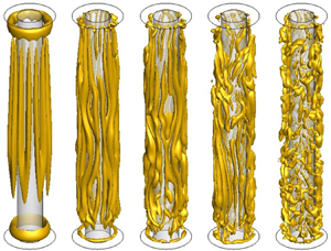
The increase of VE leads to a strong variation of longitudinal vortices (figure 14). Indeed, for VE = 4000, vortices are more branched off into several parts and become more complex. Most of the longitudinal vortices split into small ones and, for VE = 6000, they have almost disappeared from the flow pattern.

Figure 14. Instantaneous 3-D vortical structures in the annulus for high values of the electric tension: (a) VE = 4000 (Q = 20), (b) VE = 6000 (Q = 60), (c) VE = 8000 (Q = 120) and (d) VE = 10 000 (Q = 200).
Figure 15 represents time series and corresponding power spectra of the volume-averaged kinetic energy  $({E_k})$ for a few patterns, where
  $P(f)=\int_{-\infty}^{+\infty} E_{k}(t ) \exp (-2{\rm \pi} i f(t)) \,\textrm{d}t$. Figure 15(a) shows the time series of the kinetic energy of the flow for VE = 3000, illustrated in figure 13. The spectrum (figure 15b) reveals three main peaks: a peak with
  ${f_1} = 0.21$, corresponding to oscillations of columnar vortices, a peak with
  ${f_2} = 0.105$ which is a subharmonic of the previous one and a peak with
  ${f_3} = 0.08$, corresponding to low modulations induced by the presence of defects. The peak with
  ${f_4} = 0.5$ corresponds to a linear combination of
  ${f_1}$. For VE ≥ 4000, the spectra of time series (figure 15c,d) exhibit many peaks and their analysis shows that the frequency varies in time. Different studies of spatio-temporal chaotic patterns (Bot, Cadot & Mutabazi Reference Bot, Cadot and Mutabazi1998; Bot & Mutabazi Reference Bot and Mutabazi2000) have shown that frequency and wavenumber vary in time and in space. The aspect ratio used in the present study does not allow a significant spatial spectral analysis to be made.

Figure 15. Time series and power spectra of the kinetic energy  $({E_k})$ for VE = 3000 and VE = 6000. Values over the peaks are dimensionless frequencies.
3.5. Kinetic energy
The time-averaged values of the kinetic energy  ${E_k} = {\langle {\boldsymbol{u}^2}/2\rangle _V}$ has been computed for various values of VE and its variation is represented in figure 16(a). The kinetic energy of the large convective cell of the base state is almost constant for VE < 1200; the electric field does not affect the kinetic energy of the base state as it does not affect its heat flux. A weak increase is detected near the onset of columnar vortices (VE = 1200) followed by a slight decrease until VE = 2200. The decrease of the kinetic energy of columnar vortices is due to the decrease of the baroclinic axial velocity and of production of the kinetic energy by the Archimedean buoyancy (first term in the right-hand side of (2.10)). The occurrence of the regular wave flow at VE = 2500 leads to a significant increase of the time-averaged kinetic energy. The best fit of its increase with VE gives rise to the exponential growth of
  ${E_k}\ ({E_k}\sim {e^{a\cdot{V_E}}})$ with a growth rate
  $a = 2.23 \times {10^{ - 4}}$.

Figure 16. Variations with the applied electric tension VE of (a) the time-averaged kinetic energy (Ek) normalized by the kinetic energy in the absence of the electric field ( ${E_k} = 1.303$ for
  ${V_E} = 0$) and (b) different terms of the kinetic energy balance equation (2.8).
The variation of production and dissipation terms of the kinetic energy given by (2.10) is illustrated in figure 16(b). In the base state, the production of the kinetic energy by the DEP buoyancy  $( - \alpha \theta {\boldsymbol{g}_e}\boldsymbol{\cdot}\boldsymbol{u})$ is very weak and represents ~2 % of the baroclinic production
  $(\alpha \theta g{u_z})$ for VE = 1000, and it varies between 2 % and 20 % in the state of stationary columnar vortices, i.e. for
  ${V_E} \in [1200,2500[$. In that interval, the DEP buoyancy generates the axial vorticity through its coupling to the perturbations of the azimuthal temperature gradient, but the baroclinic production of the kinetic energy remains dominant. For
  ${V_E} \gt 2500$, the DEP buoyancy becomes significant and it contributes to the torque acting on the columnar vortices. The produced torque has two components: an azimuthal component due to mainly Archimedean buoyancy and an axial component due to the azimuthal component of the DEP force from the perturbative electric gravity (Yoshikawa et al. Reference Yoshikawa, Crumeyrolle and Mutabazi2013). As the electric field intensity increases, the DEP production increases while the baroclinic production decreases. The two terms become equal for
  $V_E^{\ast} = 3436$. Beyond this value, the oscillatory columnar vortices become disordered with many defects and small vortices coexisting with oscillating columnar vortices before they are completely replaced by small turbulent vortices (figure 14). The DEP force contains the electric gravity which decreases with the distance
  $({g_E}\sim {r^{ - 3}})$, favouring small vortices in contrast with the Archimedean buoyancy with constant gravity which generates the columnar vortices whose size is fixed by the length of the annulus. Moreover, the kinetic energy starts to increase significantly as shown in figure 16(a). In those states, the baroclinic production of kinetic energy becomes very weak compared to the DEP production.
3.6. Enstrophy
The enstrophy  ${\omega ^2}$ is a scalar measure of the vorticity intensity in the flow. It also represents the measure of the dissipation effects induced by vortices in the fluid. The time- and volume-averaged enstrophy
  $({\langle {\omega ^2}\rangle _{t,V}})$, normalized by that of base flow in the absence of the electric field (VE = 0), is presented for various VE in figure 17. The variation of the enstrophy reveals the same trend as that of the mean kinetic energy (figure 16a). It is almost constant in the base state (VE < 1200), it exhibits a weak decrease in the regime of stationary columnar vortices (VE ∈ [1150, 2500[), and then it exponentially grows with
  ${V_E}({\omega ^2}\sim {e^{b \cdot {V_E}}},\;b = 3.265 \times {10^{ - 4}})$ for VE > 3500. The significant increase of the enstrophy for VE > 2500 is a signature of the predominance of the production term in (2.13) by the DEP buoyancy.

Figure 17. Time- and volume-averaged enstrophy  $({\omega ^2})$ against VE. Here,
  ${\langle {\omega ^2}\rangle _V} = 121.53$ for
  ${V_E} = 0$.
4. Discussion
The base state is a flow characterized by the azimuthal vorticity generated by the temperature gradient imposed at the vertical surfaces (Bahloul et al. Reference Bahloul, Mutabazi and Ambari2000). It is destabilized by the electric field and bifurcates to the state of stationary columnar vortices with a vorticity field which can be represented as  $\boldsymbol{\omega }(r,\; \varphi ,\; z) = {\omega _b}(r){\boldsymbol{e}_\varphi } + A(t,\; z)\boldsymbol{\varOmega }(r)\cos n\varphi$, where
  ${\omega _b}(r)$ is the baroclinic vorticity of the base flow and
  $\boldsymbol{\varOmega }(r) = {\varOmega _r}{\boldsymbol{e}_r} + {\varOmega _z}{\boldsymbol{e}_z}$ is a structure vector function of the vorticity perturbation. The amplitude A(t, z) is an order parameter which satisfies the Newell–Whitehead–Segel equation with imperfection I(z) due to the asymmetric behaviour of the base flow (Cross & Hohenberg Reference Cross and Hohenberg1993):
 \begin{equation}{\tau _0}\frac{{\partial A}}{{\partial t}} = {\epsilon}A + \xi _0^{2}{\left( {\frac{{\partial A}}{{\partial y}} + \frac{1}{{2i{q_0}}}\frac{{{\partial^2}A}}{{\partial {z^2}}}} \right)^2} - l|A{|^2}A + I(z).\end{equation}
where  ${\epsilon} = ({V_E} - {V_{{E_c}}})/{V_{{E_c}}}$ is the distance from the threshold of the thermal convection,
  ${\tau _0}$ and
  ${\xi _0}$ represent the characteristic time and the coherence length of the perturbation, respectively,
  ${q_0}$ is the critical azimuthal wavenumber and l is the Landau nonlinear saturation constant. The amplitude satisfies the boundary conditions:
  $A(z = 0) = A(z = \varGamma ) = 0$. The axial vorticity of stationary columnar vortices can be chosen as an order parameter. Figure 7(c) represents a solution of (4.1) for three values of VE.
For the chosen value of the radius ratio  $\eta = 0.5$, the number of the vortices is
  $n = 14$ and corresponds to dimensionless azimuthal wavenumber
  ${q_c} = 4.67$ (Kang & Mutabazi Reference Kang and Mutabazi2019). This result significantly differs from the critical value
  ${q_c} = 3.33$, corresponding to
  $n = 10$, predicted by linear stability analysis (Meyer et al. Reference Meyer, Jongmanns, Meier, Egbers and Mutabazi2017). This suggests that the axial imperfection generates an Eckhaus-type instability and the critical wavenumber cannot be selected at the onset. The wavenumber of the stationary columnar vortices was the same for all values of
  ${V_E} \in [1200,2500[$.
The relation of (2.8) shows that the electric gravity coupled to azimuthal variation of the temperature is responsible of the creation of the axial component of the vorticity. Thus, it is the origin of the breaking of the axial invariance of columnar vortices, making them different from the Taylor columns which are axially invariant (Davidson Reference Davidson2013; Kang et al. Reference Kang, Meyer, Yoshikawa and Mutabazi2019a,Reference Kang, Meyer, Yoshikawa and Mutabazib). The coupling between the axial temperature gradient and the electric gravity gives a contribution to the azimuthal vorticity and it reinforces its axial asymmetry (figure 8b).
In the case of zero-gravity  $(g = 0)$, linear stability (Yoshikawa et al. Reference Yoshikawa, Crumeyrolle and Mutabazi2013; Meyer et al. Reference Meyer, Jongmanns, Meier, Egbers and Mutabazi2017) and DNS with periodic boundary conditions (Travnikov et al. Reference Travnikov, Crumeyrolle and Mutabazi2015) have shown that critical modes occur in the form of stationary helical vortices. We have computed the flow inside the same cylindrical annulus in the case of zero-gravity and retrieved stationary helical vortices at
  ${V_E} = 1000$ (figure 18). This value is below the critical value
  $({V_{{E_c}}} = 1150)$ for the annulus with ground gravity. Thus, the buoyancy due to the gravity g delays the onset of the thermoelectric convection and changes the helical mode into a columnar mode in agreement with the results of linear stability analysis performed in the infinite-length cylindrical annulus, as well as of experiments conducted in the same aspect ratio
  $(\varGamma = 20)$ (Meyer et al. Reference Meyer, Jongmanns, Meier, Egbers and Mutabazi2017). Furthermore, it confirms the fact that flows with small aspect system are more stable than those of large aspect ratio.

Figure 18. Helical vortices in the annulus cavity with fixed ΔT for  $g = 0$ and
  ${V_E} = 1000$. (a) Iso-surface of
  $Q = 0.5$, contours of (b) azimuthal vorticity
  $({\omega _\varphi })$ and (c) axial vorticity
  $({\omega _z})$ in a r–z plane and (d) contour of axial vorticity component
  $({\omega _z})$ at the central surface (x = 0.5).
The occurrence of oscillatory columnar vortices (zig-zag instability) as a second instability mode follows the classic scenario of the transition to spatio-temporal chaos in weakly extended systems (Manneville Reference Manneville1990; Cross & Hohenberg Reference Cross and Hohenberg1993). We have observed significant increase in the kinetic energy and in the enstrophy when the DEP production takes over the baroclinic production of the kinetic energy for VE = 3436. A similar behaviour is detected in the Nusselt number (Kang & Mutabazi Reference Kang and Mutabazi2019). Chaotic and turbulent states for  ${V_E} \gt 3500$ require more fine analysis from time signals, which needs longer time computation. This is left to a later study.
Columnar vortices obtained in the present flow configuration can be compared with columnar vortices predicted in rotating flows with a radial temperature gradient where the instability-driving force is the centrifugal buoyancy (Busse & Carrigan Reference Busse and Carrigan1974; Alonso, Net & Knobloch Reference Alonso, Net and Knobloch1995; Auer, Busse & Clever Reference Auer, Busse and Clever1995; Alonso et al. Reference Alonso, Net, Mercader and Knobloch1999; Plaut & Busse Reference Plaut and Busse2002; Ghil, Read & Smith Reference Ghil, Read and Smith2010; Kang et al. Reference Kang, Meyer, Yoshikawa and Mutabazi2019a,Reference Kang, Meyer, Yoshikawa and Mutabazib). The latter is associated with a radial effective gravity and it is the analogue of the DEP buoyancy. The two types of buoyancies are parallel to the temperature gradient and, therefore, they generate thermo-convective instabilities similar to Rayleigh–Bénard convection. To get a quantitative comparison between the two systems, we make the correspondence between the electric gravity  ${g_E}$ and the centrifugal acceleration
  ${g_{cent}} = {\varOmega ^2}\bar{R}$ where
  $\varOmega $ is the angular velocity and
  $\bar{R} = ({R_1} + {R_2})/2$ is the mean radius of the annulus. The analogue of thermal Rossby number or Hide number
  $H = \alpha \Delta TgL/{\varOmega ^2}{d^2}$ (Ghil et al. Reference Ghil, Read and Smith2010) is obtained by replacing the centrifugal acceleration by the electric gravity, i.e.
  $\tilde{H} = \alpha \Delta T\varGamma (1 + \eta )/(2Fr(1 - \eta))$, where the electric Froude number is defined as
  $Fr = {g_E}/g$, which is the analogue of the centrifugal Froude number (Lappa Reference Lappa2012). The analogue of the Taylor number
  $Ta = 4{\varOmega ^2}{d^5}/{\nu ^2}L$ reads
  $\widetilde{Ta} = (8(1 - \eta )Fr/(1 + \eta )\varGamma )Ga$, where
  $Ga = g{d^3}/{\nu ^{2}}$ is the Galileo number. The two control parameters span the so-called Hide diagram (Ghil et al. Reference Ghil, Read and Smith2010). For
  ${V_E} = 1500$, we obtain a point with coordinates
  $\tilde{H} = 0.735$ and
  $\widetilde{Ta} = 5.3386 \times {10^5}$, which belongs to the regular waves domain, while for
  ${V_E} = 6000$ we have
  $\tilde{H} = 0.74$ and
  $\widetilde{Ta} = 8.542 \times {10^7}$, which falls in the domain of irregular waves (Ghil et al. Reference Ghil, Read and Smith2010). This analogy can be used in experiments to simulate fast rotating flows using DEP forces, which can be less cumbersome and energy saving than rotating systems. The electric Froude number
  $Fr$ shows the relative effect of the DEP buoyancy compared to the gravity force. The effect of DEP buoyancy becomes significant when
  $Fr\sim 1$, and it dominates the dynamics of the flow when
  $Fr \gt 1$. The condition
  $Fr = 1$ corresponds to the value of the electric tension
  ${V_E} = 2348$, this value corresponds to the threshold of the oscillations of columnar vortices. Above this value, both the kinetic energy and the enstrophy start to grow with the electric tension
  ${V_E}$.
In our configuration, to avoid the occurrence of the baroclinic instability, we have fixed the temperature difference between cylindrical surfaces below its critical value. Thus, the Archimedean buoyancy does not drive the instability mechanism; it acts as a generator of a large convective cell.
The present study was motivated by the discrepancy between predictions of linear stability analysis and experimental results performed in parabolic flight (Dahley et al. Reference Dahley, Futterer, Egbers, Crumeyrolle and Mutabazi2011; Futterer et al. Reference Futterer, Kerbs, Plesa, Zaussinger, Hollerbach, Breuer and Egbers2013; Meyer et al. Reference Meyer, Jongmanns, Meier, Egbers and Mutabazi2017). The computed value of the threshold obtained by DNS is consistent with the experimental value with an error of 10 % (Kang & Mutabazi Reference Kang and Mutabazi2019). This big error is due to the precision of visualization technique used in experiments which has indicated an error of 18 % (Meyer et al. Reference Meyer, Jongmanns, Meier, Egbers and Mutabazi2017). Moreover, the visualization by shadowgraph technique suggests the existence of columnar vortices (Meyer et al. Reference Meyer, Jongmanns, Meier, Egbers and Mutabazi2017) while the PIV technique shows vortices in the (r, z) plane suggesting the existence of helical vortices (Dahley et al. Reference Dahley, Futterer, Egbers, Crumeyrolle and Mutabazi2011; Futterer et al. Reference Futterer, Kerbs, Plesa, Zaussinger, Hollerbach, Breuer and Egbers2013). This difference comes from the fact that the shadowgraph technique performs an integration of data along the axial direction. The PIV data reported in Dahley et al. (Reference Dahley, Futterer, Egbers, Crumeyrolle and Mutabazi2011) have been determined away from the onset so that observed cross-sections of vortices may correspond to disordered vortices. The present DNS results will be of help in the preparation of the next campaigns of parabolic flight experiments and in the sounding rocket.
In the present study, we have assumed that the working fluids are perfect dielectrics, and we have neglected the dielectric heating. This assumption holds for non-polar dielectrics which have a small loss tangent under typical experimental conditions. For polar fluids (e.g. 1-Nonanol), the polarization under a high-frequency electric field occurs with a phase delay and the dielectric heating cannot be neglected since it can lead to flow patterns (Zaussinger et al. Reference Zaussinger, Haun, Neben, Seelig, Travnikov, Egbers, Yoshikawa and Mutabazi2018).
5. Conclusion
A flow of a dielectric fluid confined in a cylindrical annulus with a short aspect ratio subjected to a high-frequency electric field and a fixed temperature difference between cylinder walls has been investigated numerically. The temperature difference was chosen below its critical value in order to avoid instability of the large convective cell in the absence of electric field. The intensity of the electric tension  $({V_E})$ imposed on two cylinders has been progressively increased from zero in order to influence the DEP force on the velocity and temperature fields. The DEP force leads to the onset of stationary counter-rotating columnar vortices. Velocity and temperature fields have a pronounced axial dissymmetry. The increase of the electric field intensity leads to oscillatory vortices, which are then broken into small turbulent vortices for larger values of the electric tension. The kinetic energy and the enstrophy of the different states have been computed; they both increase with the electric field intensity when the production of the kinetic energy by the DEP buoyancy overcomes the production by the Archimedean buoyancy.
Acknowledgements
The present work has benefited from the financial support from the French Space Agency (CNES, project INTEHLDI) and of the French National Research Agency (ANR) through the program ‘Investissements d'Avenir (N°ANR-10 LABX-09-01)’ LABEX EMC3. C.K. was supported by the project BIOENGINE of the CPER-FEDER Normandie. Computations presented in this work have been performed using resources provided by CRIANN (Normandy, France).
Declaration of interests
The authors report no conflict of interest.
Supplementary material
Supplementary material is available at https://doi.org/10.1017/jfm.2020.843.


