The EGSnrc simulation code

The EGSnrc code system (Electron-Gamma Shower)Reference Kawrakow and Rogers^5,Reference Kawrakow⁶ is a general purpose Monte Carlo code system used for the simulation of the coupled transport of electrons and photons through an arbitrary geometry. It is an improved version of its predecessor, the EGS4Reference Ford and Nelson^7–Reference Nelson, Rogers, Jenkins, Nelson and Rindi⁹ system with significant advances in several aspects of electron transport: new electron transport algorithm PRESTA-II, improved multiple-scattering theory which includes relativistic spin effects in the cross section, electron impact ionisation, more accurate boundary crossing algorithm, and improved sampling algorithms for a variety of energy and angular distributions. The detailed description of these features of the EGSnrc system can be found in the EGSnrc manualReference Kawrakow and Rogers⁵ and the manual for the multi-platform version of the EGSnrc system.Reference Kawrakow, Mainegra-Hing and Rogers¹⁰

Both the EGS4 and the EGSnrc systems are well-structured and thoroughly documented programs, which allow the user to simulate electromagnetic cascade showers in any material. Examples of the usage of the codes in medical radiation physics applications are given in the literature.Reference Kilic^11–Reference Taylor and Rogers²¹

In the EGSnrc code, the user writes:

1. 1. a code to handle input, output and initialisation of various parameters;

2. 2. a subroutine to specify the geometry of the particular problem;

3. 3. a scoring routine which keeps track of the quantities of interest (in this case the energy deposited in the active detector volume).

The EGSnrc code consists of two distinct components: the PEGS4 preprocessor and the EGSnrc simulation code. PEGS4 creates data sets for each element, compound or mixtures used in the simulation, which are read in by the HATCH routine of the EGSnrc code itself. The user is responsible for writing four routines, MAIN, HOWNEAR, HOWFAR and AUSGAB, which form what is known as the user-code. MAIN performs any initialisation necessary for the simulation, including the media to be used, particle parameters and cut-off energies. The latter three determine the geometry and output (scoring) of the simulation, respectively. Having directed HATCH to obtain media data sets, MAIN then repeatedly calls SHOWER, once for each incident particle. SHOWER and its various subroutines simulate the particle and its offspring until they leave the region of interest, reach the end of their track or are discarded.

The user-code TRANSMIT used in this work consists of a main program and several subroutines which use the EGSnrc system to simulate transmission of megavoltage x-rays through different attenuating materials. A separate program called PEGS handles the preparation of the data files required for a particular set of materials.

The simulation geometry

In this work, the Monte Carlo simulations were carried out using the geometry shown in Figure 1. The detector was located on the z-axis of a Cartesian coordinate system (x,y,z) at a distance of 200 cm from the x-ray source which was assumed to be at the origin. In these calculations, the efficiency of this detector is taken as unity. The distance between the source and the attenuating material was 100 cm. The irradiation field size was 4 × 4 cm² at the point 100 cm from the source. The simulations were performed for the three different attenuating materials with 4, 6 and 10 MV x-ray beams. The 4 MV x-ray spectrum was obtained from the Mitsubishi EXL15DP linear accelerator manufacturer data (Mitsubishi Electric Corporation, 2-2-3, Marunouchi, Chiyoda-ku, Tokyo 100-8310, Japan) whereas the 6 and 10 MV x-ray spectra were obtained from the Varian 2100C linear accelerator manufacturer data (Varian Associates Inc., Oncology Systems, 3045 Hanover St., Palo Alto, CA 94304-9910). Ten runs each having 100 million photons were used in each simulated transmission. This was necessary to limit the maximum error in the scoring region of 0.5%. An example of a user-code written for the simulation of x-ray transmission through lead is given in Appendix 1.

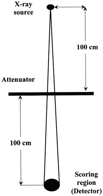
Figure 1. A schematic diagram of the simulation geometry.

The user-code TRANSMIT was implemented with several variance reduction techniques to accelerate the simulation. These included photon forcing, bremsstrahlung splitting and range rejection. The techniques of selective bremsstrahlung splitting (SBS) and range rejection were used in the simulation of the linear accelerator head. In bremsstrahlung splitting, each bremsstrahlung event produced not one but N photons (N > 1, set by user). Each bremsstrahlung photon had a weight 1/N. The splitting parameter, N, is a constant throughout the simulation in uniform bremsstrahlung splitting (UBS), but varies greatly when SBS is used. In SBS, the probability of photon emission into the treatment field for a known electron direction and energy is calculated once at the beginning of the simulation using the bremsstrahlung cross section. Then the information is used on-the-run to determine how often a bremsstrahlung event should be re-sampled to maximise the efficiency of photon-related end-points of interest, such as fluence. Rogers et al.Reference Rogers, Ma, Walters, Ding, Sheikh-Bagheri and Zhang²² stated that SBS can increase efficiency by an additional factor of 3–4 compared with the UBS. They found that a maximum N value, N _max, between 200 and 1000 is appropriate, and that the minimum value, N _min, should be set to 0.1 N _max to obtain the optimum gain in efficiency. In this study, the N _max and N _min were set to 200 and 20, respectively. Range rejection was also used to reduce simulation time. The basic method was to calculate the range of a charged particle and terminate its history (depositing all of its energy at that point) if it cannot leave the current region or cannot reach the score plane. The range is calculated using restricted stopping power, and accordingly represents the longest possible range for a given cutoff energy. The range rejection energy was set to 3.0 MeV.

Narrow beam geometry

The simulation results of percent transmission versus attenuator thickness are illustrated in Figures 2–4 for narrow beam geometry. The graphs illustrate that the simulated data are essentially exponential. Table 1 compares the calculated linear attenuation coefficients and half-value layers from the simulations with the experimentally measured results of Tajiri et al.Reference Tajiri, Sunaoka, Fukumura and Endo⁴ The simulated narrow beam attenuation coefficients in this work were derived by performing a least-squares fit to the simulated results using the equation:

(1)

Figure 2. X-rays transmission curves through Lipowitz’s metal.

Figure 3. X-rays transmission curves through lead attenuator.

Figure 4. X-rays transmission curves through Rad-block attenuator.

Table 1. The narrow beam linear attenuation coefficients (in cm⁻¹) and HVL (in cm) of the three different attenuating materials

HVL, half-value layer.

where I is the intensity (energy fluence) of radiation after positioning an absorber in the beam, I _o is the intensity of radiation for no absorber in the beam, μ is the linear attenuation coefficient in cm^–1 and x is the thickness of the absorber in cm. The simulated attenuation coefficients obtained in this work agreed with the experimentally measured values to an average of 3.3% with a maximum deviation of 4.4% occurring for the 10 MV x-ray beam with a Lipowitz’s metal attenuator.

The comparison between the attenuation properties of the three materials shown in Table 1 revealed also the shielding ability of Lipowitz’s metal. These findings prove that this material has the least radiation transmission. In addition, the low fusion temperature of about 70 °C of Lipowitz’s metal enables casting of the material at radiotherapy centres.

Table 2 shows the percentage deviation between the experimental and simulation values of the linear attenuation coefficients of Lipowitz’s metal, lead and Rad-block attenuators for the different megavoltages x-ray beams. The deviation between the experimental and simulation results was calculated as follows:

(2)

Table 2. The percentage deviation between experimental and simulation values of the narrow beam linear attenuation coefficients for the three different attenuating materials

where μ _exp and μ _sim are the experimental and simulated linear attenuation coefficients, respectively. Considering the variations in x-ray spectra used for the experimental measurements,Reference Tajiri, Sunaoka, Fukumura and Endo⁴ the EGSnrc Monte Carlo routine TRANSMIT as applied here yields reasonable estimates of the megavoltage x-ray transmission through the three different attenuators.

Figures 5–7 demonstrate plots of thickness against the expected transmission through the three materials investigated at 4, 6 and 10 MV, respectively. Such curves are instructive and can be used for radiation shielding calculations (e.g., wall thickness calculations of medical linear accelerator bunkers). Usually, medical linear accelerator bunkers are designed using basic shielding calculations. These calculations are dependent on the transmission of x-ray and gamma-ray through different shielding materials measured at different megavoltages. In our study, data from Figures 5–7 can be used to obtain the tenth value layer of the shielding materials. These values could then be used in the original calculation to work out the exact thickness of the required shielding material and its cost. Examples on how to use transmission data in the calculation of wall thickness of the linear accelerator bunker are given in refs 23 and 24.

Figure 5. % Transmission through lead, Lipowitz and Rad-block materials investigated at 4 MV.

Figure 6. % Transmission through lead, Lipowitz and Rad-block materials investigated at 6 MV.

Figure 7. % Transmission through lead, Lipowitz and Rad-block materials investigated at 10 MV.

Broad beam geometry

The results of the narrow beam simulations obtained in this study were used to determine broad beam attenuation coefficients. Broad beam geometries are complicated by radiation that is scattered from the absorber and reaches the detector. The effects of first scatter can be calculated analytically by using the expressions given by Attix.Reference Attix²⁵ The ratio of scatter-to-primary intensity is given by:

(3)

where S represents the first-scatter intensity, N _e is the number of electrons/cmReference el-Khatib, Podgorsak and Pla³ in the absorber, x _o is the absorber thickness in cm, and σ _o is the integrated cross section for the energy of the photons scattered between 0° and the maximum scattering angle and is given in cm². This later quantity is a complicated function of incident energy and the maximum scattering angle and is given in Attix.Reference Attix²⁵

If it is assumed that broad beam attenuation is also exponential, then:

(4)

where I _b is the broad beam intensity below the absorber and μ _b is the effective linear attenuation coefficient for the broad beam geometry, and is given by:

(5)

where S/I can be determined from Eq. (3). Although the assumption of exponential attenuation in broad beams is not necessarily valid, the variation of μ _b as a function of radiation field size and absorber thickness will give an indication of the variation in attenuation as a function of these parameters. The spectrum of photon energies from the linear accelerators complicates this calculation for high-energy x-rays. However, by using previously determined spectra for 4, 6 and 10 MV x-rays, broad-beam attenuation coefficients can be determined using a weighted averaging procedure:

(6)

where T represents the total number of photons at energy E and the integral is considered over the total energy spectrum. Tables 3–5 illustrate the narrow- and broad-beam attenuation coefficients for the 4, 6 and 10 MV x-rays. Broad-beam geometries calculations were performed for a variety of field sizes (10 × 10 cm², 20 × 20 cm² and 40 × 40 cm²) using the three different attenuators. It is clear from the data that the broad beam attenuation coefficients decreased with increased field size and photon energy. For Lipowitz’s metal, the difference in the linear attenuation coefficient data between the broad beam attenuation coefficient and the narrow-beam value lies between 3.6% and 20% depending on x-ray energy and field size. Similarly, the difference between the broad-beam attenuation coefficient and the narrow-beam value for lead material lies between 1.5% and 10.4%. For the Rad-block material, the difference lies between 0.53% and 6.8%. This appears to be reasonable in view of the scatter within the source as well as the various scattering materials in the beam. The relative transmission of megavoltage x-rays through the three different absorbers varies considerably as a function of field size and x-ray energy. Although this has been well known for many years and has been considered for radiation protection purposes, virtually no quantitative data exist for therapeutic geometries. It is noticeable from the data of Tables 3–5 that the broad-beam attenuation coefficient values decreased with increasing photon energy and effective atomic number of the attenuating material. This raises the question: What is the clinical significance of this, and should these variations be considered in clinical dosimetry? Narrow beam measurements are not always easy to perform in a clinical environment, hence a simplified procedure would be useful. An empirical approach is to measure broad-beam attenuation coefficients for three field sizes (e.g., 10 × 10 cm², 20 × 20 cm² and 40 × 40 cm²) and to calculate a linear least squares fit to these data as a function of side of square field. Because a change in geometry will result in a change in attenuation coefficient as a function of field size, plotting the attenuation coefficient as a function of maximum scattering angle allows for a more general representation and should provide attenuation coefficients for any clinical geometry.

Table 3. Narrow and broad beam linear attenuation coefficients (in cm⁻¹) for Lipowitz’s metal

Table 4. Narrow and broad beam linear attenuation coefficients (in cm⁻¹) for lead

Table 5. Narrow and broad beam linear attenuation coefficients (in cm⁻¹) for Rad-block

The theoretical first scatter calculations are useful for predicting the qualitative trends and demonstrate quantitative agreement with measured results. The variation in attenuation coefficient as a function of field size extends beyond the range of errors allowed for clinical dosimetry and under many clinical conditions, field-size dependent attenuation coefficients should be used.